HAL Id: hal-02295157
https://hal.archives-ouvertes.fr/hal-02295157
Submitted on 24 Sep 2019
HAL is a multi-disciplinary open access
archive for the deposit and dissemination of
sci-entific research documents, whether they are
pub-lished or not. The documents may come from
teaching and research institutions in France or
abroad, or from public or private research centers.
L’archive ouverte pluridisciplinaire HAL, est
destinée au dépôt et à la diffusion de documents
scientifiques de niveau recherche, publiés ou non,
émanant des établissements d’enseignement et de
recherche français ou étrangers, des laboratoires
publics ou privés.
Sensor Displacement Estimation
Javier Minguez, Luis Montesano, Florent Lamiraux
To cite this version:
Javier Minguez, Luis Montesano, Florent Lamiraux. Metric-Based Iterative Closest Point Scan
Match-ing for Sensor Displacement Estimation. IEEE Transactions on Robotics, IEEE, 2006, 22 (5),
pp.1047-1054. �10.1109/TRO.2006.878961�. �hal-02295157�
Metric-Based Iterative Closest Point
Scan Matching for Sensor Displacement Estimation
Javier Minguez Luis Montesano Florent Lamiraux
Abstract— This paper addresses the scan matching problem
for mobile robot displacement estimation. The contribution is a new metric distance and all the tools necessary to be used within the Iterative Closest Point framework. The metric distance is defined in the configuration space of the sensor and takes into account both translation and rotation error of the sensor. The new scan matching technique ameliorates previous methods in terms of robustness, precision, convergence and computational load. Furthermore, it has been extensively tested to validate and compare this technique with existing methods.
Index Terms— Scan matching, Sensor Displacement
Estima-tion, Mobile Robots.
I. INTRODUCTION
A
Key issue in autonomous mobile robots is to keep trackof the vehicle position. One strategy is to estimate the robot displacement using successive range measurements. This problem is usually denoted as scan matching. Many applications in robotics such as mapping, localization or tracking use these techniques to estimate the relative robot displacement [1], [2], [3], [4], [5]. In this paper, we propose a new geometric 2D scan matching approach that has been extensively evaluated and compared with the most widely used techniques.
The objective of the scan matching techniques is to compute the relative motion of a vehicle between two consecutive configurations by maximizing the overlap between the range measurements obtained at each configuration. More precisely,
given a reference scan Zref, the new scan Znew and a
rough estimation q0 of the relative displacement of the
sen-sor between the scans, the objective is to estimate the real displacement q = (x, y, θ) between them.
One of the main differences between the existing algorithms is the usage or not of high-level entities such as lines or planes. On the one hand, in structured environments, one can assume the existence of polygonal structure in the environment [6], [7], [8]. These methods are fast and work quite well for indoor environments. However, they limit the scope of application to the extraction of geometric features that are not always available in unstructured environments.
On the other hand, a great deal of work has been done to perform in any type of scenario dealing with raw data. Roughly, these techniques are based on an iterative process that estimates the sensor displacement that better explains the overlap between the scan measurements. For example,
J. Minguez and L. Montesano are with the Dpto. de Informática e Ingeniería de Sistemas, Universidad de Zaragoza (Spain). E-mail: jminguez,[email protected] .
F. Lamiraux is with the LAAS-CNRS (France). E-mail: fl[email protected] .
[9] constructs a piecewise continuous differentiable density that models on a grid the probability to measure a point, and then, apply the Newton’s algorithm. By converting the scans to statistical representations, [10] iteratively computes the cross-correlation that results in the displacement. In [11] the motion parameters are estimated using a constrained velocity equation for the scanned points. However, the most popular methods usually follow the Iterative Closest Point (ICP) algorithm [12] (see [13] for variants of the original method). The ICP algo-rithm addresses this problem with an iterative process in two steps. At each iteration k, there is a search of correspondences
between the points of both scans (Zref and Znew). Then, the
estimation of relative displacement q0 is improved through a
minimization process until convergence. More precisely, let pi
with i = 1 . . . n and rj with j = 1 . . . m be the points of Zref
and Znew respectively, and qk = q0. Repeat:
1) For each pi in Zref compute the closest point in Znew
(transformed to the system of reference Zref using the
estimation qk) whose distance is lower than a given
threshold dmin:
ci= arg min
rj
{d(pi, qk(rj))and d(pi, qk(rj)) < dmin}
(1)
The result is a set of l correspondences C = {(pi, ci) | i = 1 . . . l}.
2) Compute the displacement estimation qmin that
mini-mizes the mean square error between pairs of C:
Edist(q) =
l
�
i=1
d(pi, q(ci))2 (2)
Let be qsol = qmin ⊕ qk. If there is convergence
the estimation is qsol, otherwise we iterate again with
qk+1= qsol.
A common feature of most ICP versions is the usage of the Euclidean distance to establish the correspondences and to apply the least squares [14], [15], [16]. However, as pointed out by [17], the limitation of this distance is that it does not take into account the sensor rotation. Following the example outlined by [17], in Figure 1 we show how with Euclidean distance, points far from the sensor could be far from its correspondent due to rotations of the sensor, and how the associations could not clearly explain the motion (again due to rotations). We understand that this is a central problem of the ICP algorithms: to find a way to measure (to find the closest correspondent and to apply the minimization) in such a way that it captures the sensor translation and rotation at the same time. In order to overcome this limitation [17]
Sref
Snew
Points of S Points of Srefnew
−4 −3 −2 −1 0 1 2 3 4 −3 −2 −1 0 1 2 3 m m Sref Snew −5 0 5 −3 −2 −1 0 1 2 3 m m Sref Snew (a) (b)
Fig. 1. (Top) The distance between the same points become larger in terms of Euclidean distance with a rotation displacement, which makes difficult the association. (Bottom) An ellipsoid rotated. (a) The associations using Euclidean distance do not clearly explain the rotational motion, which would affect convergence. (c) With the new distance this rotational motion is captured.
proposed to compute two sets of correspondents, one by the Euclidean distance and the other one by a range rule (to capture the sensor rotation). This strategy ameliorates the ICP behaviour facing sensor rotations. However, it employs two parallel minimizations of two different criteria to get the coordinates of a single variable (translation with one minimization and rotation with the other). Thus, some minima could arise due the composition of the coordinates, mainly affecting the robustness and precision of the method.
Our contribution resides in the definition of a new distance measure in the sensor configuration space that takes into account both translation and rotation at the same time. By only modifying the way to measure in the ICP framework, translation and rotation are compensated simultaneously in all the steps of the method. As a consequence, the results ameliorate previous methods in terms of robustness, precision, convergence and computational load. An added value of this research is the strong experimental component carried out to validate and compare this technique with existing methods.
The paper is distributed as follows: in Section II-B we describe the metric distance and we express the least square criterion based on this distance measure. In Section III, we discuss the experimental results and we compare our method with existing methods. Finally, we discuss and draw our conclusions in Section IV.
II. DISTANCEMEASURE ANDMINIMIZATION
In this section, we introduce first our distance measure in the plane and next we describe the minimization.
A. Distance point to point
A rigid body transformation in the plane is defined by a vector q = (x, y, θ) representing the position and orientation
(−π < θ < π) of the scanner sensor in the plane. We define the norm of q as :
�q� =�x2+ y2+ L2θ2 (3)
where L is a positive real number homogeneous to a length.
Given two points p1 = (p1x, p1y) and p2 = (p2x, p2y) in
R2, we define a distance between p
1 and p2 as the minimum
norm among the rigid body transformations that move a point to another:
dp(p1, p2) = min{�q�such that q(p1) = p2} (4)
where q(p1) = � x + cos θ p1x− sin θ p1y y + sin θ p1x+ cos θ p1y � (5)
It can be easily checked that dp is a real distance satisfying
for any p1 and p2:
1) dp(p1, p2) = dp(p2, p1)
2) dp(p1, p2) = 0implies p1= p2
3) dp(p1, p3) ≤ dp(p1, p2) + dp(p2, p3)
Unfortunately, there is no closed form expression of the above distance w.r.t. the coordinates of the points. However, we can compute a valid approximation when the minimum norm transformation is small, by linearizing (5) about θ = 0. The
set of rigid-body-transformations satisfying q(p1) = p2can be
approximated by the set of solutions (x, y, θ) of the following system:
x + p1x− θ p1y= p2x
y + θ p1x+ p1y= p2y
The set of solutions is infinite and can be expressed by:
x = p2x− p1x+ θ p1y
y = p2y− p1y− θ p1x
where θ is a parameter for the set of solutions. Let us recall that according to (4), we need to find the solution that minimizes the norm of q = (x, y, θ). For a given θ, this norm is given by the following equation, after substituting the above expressions of x and y into (3):
�q�2= (δx+ θ p1y)2+ (δy− θ p1x)2+ L2θ2
where δx = p2x− p1x and δy = p2y − p1y. Expanding the
above expression, we obtain a polynomial of degree 2 in θ:
�q�2= aθ2+ bθ + c
with a = p2
1y+p21x+L2, b = 2(δxp1y−δyp1x)and c = δx2+δ2y.
Notice that a > 0 implies that this expression has a unique minimum for θ = −b/(2a) and the value of this minimum is given by �ˆq�2 = −b 2+ 4ac 4a = −(δxp1y− δyp1x)2+ (p1y2 + p21x+ L2)(δx2+ δ2y) p2 1y+ p21x+ L2 = δ2 x+ δ2y− (δxp1y− δyp1x)2 p2 1y+ p21x+ L2
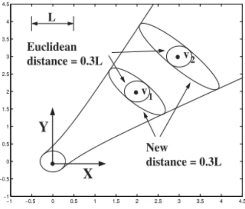
−1 −0.5 0 0.5 1 1.5 2 2.5 3 3.5 4 4.5 −1 −0.5 0 0.5 1 1.5 2 2.5 3 3.5 4 4.5 Euclidean distance = 0.3L 1 v New L distance = 0.3L X Y 2 v
Fig. 2. Iso-distance curves of dap
p for two points v1and v2.
Finally, the approximated distance between p1 and p2 is:
dapp (p1, p2) = � δ2 x+ δy2− (δxp1y− δyp1x)2 p2 1y+ p21x+ L2 (6)
So as to better understand the properties of this distance measure, let us compute the iso-distance curves. Again, we do not have the exact expression of the iso-distance curves but, if we use approximation (6), we can prove that the
iso-distance curves relative to dap
p :
{p2∈ R2 such that dapp (p1, p2) = c}
are ellipses centred on p1 with principal axes (p1x, p1y) and
(−p1y, p1x) and lengths c and c
�
1 + �p1�2
L2 (see Figure 2).
Furthermore, their dimensions depend on ||p1|| and the value
of L. In fact, L balances the trade-off between translation and rotation. Notice that when L → ∞, the new distance tends to the Euclidean distance (the iso-distance surfaces of the Euclidean distance are spheres).
The iso-distance curves hold the Euclidean distance in the
(p1x, p1y)axis. However, in the rest of the space, the distance
is smaller than the Euclidean distance, since the latter is the
norm of the translation between p1 and p2 and therefore is
bigger than the minimum norm. Furthermore, the iso-distance
curves become larger but only in the (−p1y, p1x)axis as the
point p1 is further from the sensor location, which captures
the sensor rotation (see Figure 1). This distance is used in expression (1) in order to establish the correspondences. Figure 1b depicts the associations in the ellipsoid example and some iso-distance curves over-imposed.
B. Least Square Minimization
The next step is to compute the q that minimizes expression (2) but in terms of the new distance. Expression (2) with distance (6) leads to:
Edist(q) = n � i=1 � δix2 + δiy2 − (δixpiy− δiypix)2 p2 iy+ p2ix+ L2 � (7) where δix = cix− ciyθ + x − pix δiy = cixθ + ciy+ y − piy (7) is quadratic w.r.t. q: Edist(q) = qTAq + 2bTq + c
where c is a constant number, A is a symmetric matrix A = aa1112 aa1222 aa1323 a13 a23 a33 a11=�ni=11 − p2iy ki a12=�ni=1 pixpiy ki a13=�ni=1−ciy+pkiyi (cixpix+ ciypiy) a22=�ni=11 − p2ix ki a23=�ni=1cix−pkixi(cixpix+ ciypiy) a33=�ni=1c 2 ix+ c2iy−k1i(cixpix+ ciypiy)2 and b = �n i=1cix− pix− piy ki(cixpiy− ciypix) �n i=1ciy− piy+pkixi (cixpiy− ciypix) �n i=1[ 1 ki(cixpix+ cixpiy) − 1](cixpiy− ciypix)
where ki = p2ix+ p2iy+ L2. The value of q that minimizes
Edist(q)is thus
qmin= −A−1b
In summary, we have described in this Section all the mathematical tools in order to introduce the new metric in the ICP formalism. We outline next the experimental results.
III. EXPERIMENTALRESULTS
We tested the method with real data obtained with a Sick laser scanner mounted on a robotic wheelchair. This sensor
has a field of view of 180◦, a maximum range of 8.1m and
with a frequency of 5Hz it gathers 361 points. We carried out the computations on a Pentium IV 1.8Ghz.
In order to compare the new method (metric-based ICP, MbICP in short) with existing scan matching techniques, we used the standard ICP and the widely known IDC algorithm [17]. The IDC algorithm uses two types of correspondences (Euclidean distance and a range rule) and two minimizations to estimate the translation and rotation of the sensor. In the IDC implementation, we have been using [3], [5], we reject outliers using visibility criteria [17] and range criterions [14]. We use a trimmed version of the ICP to manage the corre-spondences [18] that improves the least squares minimization, and a smooth criterion of convergence [14]. Furthermore, as suggested by [17], we interpolate between successive range points (local structure) to compute the correspondences. We also implemented these features in the ICP and the MbICP algorithm (we give the expression of the distance point to segment in the Appendix to interpolate with the new metric). In order to show a fair comparison, we used the same values for common parameters (we used our IDC previous parameters for the ICP and MbICP). We only tuned the metric length L in the MbICP (in section IV we discuss how to do it). As criteria of convergence (Section I), we set a maximum number
of iterations to 500, an error ratio below 10−4 and sensor
displacement qmink < (10
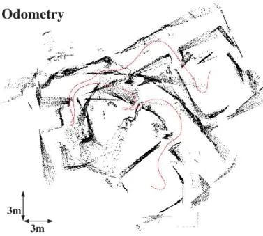
Odometry
3m 3m
Fig. 3. Data set collected in a trial of 100m
The experiments discussed next are based on a set of data collected with a robotic wheelchair in our laboratory (a travel of 100m with 780 different scans). The idea was to have, in the same data set, scenarios with very different nature that cover the most representative indoor environments such as rooms full of furniture, open corridors, or windows and walls with glass (the nature varies from open/dense, structured/unstructured, etc). All these issues were present in our data set (Figure 3). We describe next two types of experiments. In the first one we study the properties of the algorithms such as robustness, pre-cision, convergence rate and computational load. The second one consists in the reconstruction of the environment using the visual odometry provided by the result of the scan matching of consecutive scans.
The objective of the first experiment was to study the robust-ness, precision, convergence rate and computational load of each algorithm. In order to do it, we matched each scan against itself using random initial locations. Thus, we know the exact ground truth (0, 0, 0) and we can compare the performance of the three algorithms. We carried out six collections of experiments with the initial location error ranging from 0.05m
in x and y, and 2◦ in θ (Experiment 1) up to 0.2m in x and
y, and 45◦ in θ (Experiment 6), see Table I. We repeated the
procedure 100 times for each scan which makes 78000 runs for experiment, and a total of 624000 runs (6 experiments) for each method.
We discuss first the results in terms of robustness. A run was considered a failure when the solution was larger than
0.05m in translation and 0.05rad (2.86◦) in rotation (notice
that the ground truth is (0, 0, 0)). These values are just a threshold used to identify failures of the method. Those solutions with an error lower than the threshold are analysed in the precision study of the method. Regarding robustness, for
these techniques, the more representative characteristics are the True Positives (the method converged to the right solution) and the False Positives (the method converged but to a wrong solution). The True Negatives correspond to cases where the algorithm did not converge (after the maximum number of iterations) and the solution was wrong. In the False Negatives the algorithm did not converge and the solution was correct. Notice that negative are always preferable than having false positives. Table I summarizes the results.
TABLE I
MBICPVSIDCANDICP (ROBUSTNESS)
Method MbICP IDC ICP
Robustness (%) (%) (%)
True Positives 100.0 100.0 100 Experiment 1 False Positives 0.0 0.0 0.0 (0.05m, 0.05m, 2◦) True Negatives 0.0 0.0 0.0
False Negatives 0.0 0.0 0.0 True Positives 100.0 99.997 100 Experiment 2 False Positives 0.0 0.0 0.0 (0.1m, 0.1m, 4◦) True Negatives 0.0 0.0 0.0
False Negatives 0.0 0.025 0.0 True Positives 100.0 99.61 100.0 Experiment 3 False Positives 0.0 0.015 0.0 (0.15m, 0.15m, 8.6◦) True Negatives 0.0 0.019 0.0
False Negatives 0.0 0.003 0.0 True Positives 100 99.375 99.981 Experiment 4 False Positives 0.0 0.365 0.107 (0.2m, 0.2m, 17.2◦) True Negatives 0.0 0.079 0.001
False Negatives 0.0 0.179 0.0 True Positives 99.719 96.73 97.147 Experiment 5 False Positives 0.279 1.876 2.632 (0.2m, 0.2m, 34.3◦) True Negatives 0.001 1.176 0.220
False Negatives 0.0 0.214 0.0 True Positives 99.248 92.01 94.198 Experiment 6 False Positives 0.728 4.09 5.473 (0.2m, 0.2m, 45◦) True Negatives 0.023 3.23 0.315
False Negatives 0.0 0.65 0.012
For all methods, the true positives decrease and the false positives increase as the errors increase (Experiments 1 to 6). This means that the robustness of the methods decrease as the errors increase. We observe that the MbICP has the best performance, since the percentage of true positives is higher and the false positives lower than the other methods. Furthermore, MbICP behaves well even in the most demanding experiment (Experiment 6) with a rate higher than 99% and lower than 1% of true and false positives respectively. Regarding the IDC and ICP, we observe that although IDC has a lower rate of true positives than ICP, it has less false positives indicating better robustness.
In order to address precision, we separated the percentage of trials that achieved a given range of accuracy. A solution
with less than 10−3 of error in all the coordinates (m,m,rad)
achieved maximum precision, while an error larger than 0.05m or 0.05rad indicates an error. Table II summarizes the results. We observe that the precision of the MbICP is better than the other methods. If one discards the failures of the IDC and ICP (error > 0.05m or > 0.05rad) and relax the precision ranges, the precision of the MbICP and ICP is similar and slightly better than the IDC. Furthermore, for all methods, the precision remains constant while the errors increase (from Experiment 1 to 6). Notice that the precision is very related
TABLE II
MBICPVSIDCANDICP (PRECISION)
Method MbICP IDC ICP
Precision (m,rad) (%) (%) (%) < 0.001 81.27 83.315 57.78 (0.001, 0.005) 18.72 16.682 42.219 Experiment 1 (0.005, 0.01) 0.0 0.0 0.0 (0.05m, 0.05m, 2◦) (0.01, 0.05) 0.0 0.002 0.0 > 0.05 0.0 0.0 0.0 < 0.001 80.97 83.118 57.51 (0.001, 0.005) 19.02 16.844 42.48 Experiment 2 (0.005, 0.01) 0.0 0.0 0.0 (0.1m, 0.1m, 4◦) (0.01, 0.05) 0.0 0.032 0.0 > 0.05 0.0 0.0 0.0 < 0.001 80.84 82.952 56.62 (0.001, 0.005) 19.15 16.965 43.37 Experiment 3 (0.005, 0.01) 0.0 0.0 0.0 (0.15m, 0.15m, 8.6◦) (0.01, 0.05) 0.0 0.047 0.0 > 0.05 0.0 0.034 0.002 < 0.001 81.28 81.96 56.30 (0.001, 0.005) 18.71 16.795 43.58 Experiment 4 (0.005, 0.01) 0.0 0.0 0.0 (0.2m, 0.2m, 17.2◦) (0.01, 0.05) 0.0 0.799 0.0 > 0.05 0.0 0.444 0.10 < 0.001 80.92 79.537 54.00 (0.001, 0.005) 18.79 16.357 43.13 Experiment 5 (0.005, 0.01) 0.0 0.041 0.00 (0.2m, 0.2m, 34.3◦) (0.01, 0.05) 0.0 0.811 0.00 > 0.05 0.28 3.052 2.85 < 0.001 80.38 74.94 52.184 (0.001, 0.005) 18.864 16.53 42.01 Experiment 6 (0.005, 0.01) 0.0 0.37 0.0 (0.2m, 0.2m, 45◦) (0.01, 0.05) 0.0 0.81 0.01 > 0.05 0.751 7.32 5.78
to the convergence criteria. One could think that the results should vary with stricter criteria. We carried out also these tests and all the methods improved precision. However, the tests revealed a problem of the IDC regarding precision and independent of the convergence criteria (we discuss this topic in section IV).
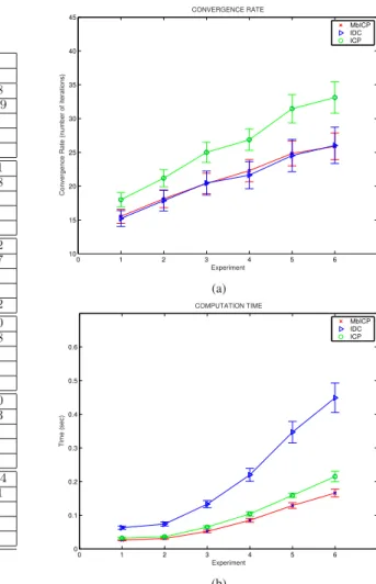
The convergence rate is the number of iterations until convergence (we only used the true positives for this study). Figure 4a shows the mean and the standard deviation of the number of iterations for each method and experiment. Notice how the MbICP and IDC are very similar but both faster than the ICP. This result agrees with [17] (IDC), which pointed out the fact that taking into account rotation improves the convergence rate of the ICP.
Figure 4b shows the execution times of each method. The MbICP is in average the fastest algorithm followed by the ICP and IDC. Although the MbICP and IDC have similar convergence rates, the execution time of the MbICP is much lower, due to the fact that the IDC algorithm establishes two different sets of correspondences and performs two min-imizations at each step (increasing computation time). For all methods, the computational load increases with the error (from Experiment 1 to 6). However, the time is not proportional to the number of iterations. This is because the IDC needs a maximum angular region to search correspondences for each point [17]. The MbICP and ICP do not need this parameter, but we used it to accelerate the algorithm and therefore having a fair comparison with the IDC times. This parameter (region
0 1 2 3 4 5 6 7 10 15 20 25 30 35 40 45 CONVERGENCE RATE Experiment
Convergence Rate (number of iterations)
MbICP IDC ICP (a) 0 1 2 3 4 5 6 7 0 0.1 0.2 0.3 0.4 0.5 0.6 COMPUTATION TIME Experiment Time (sec) MbICP IDC ICP (b)
Fig. 4. (a) Mean and 0.2 times the standard deviation of the convergence rate and (b) mean and 0.2 times the standard deviation of the execution time.
of correspondences) has to be increased as the errors increase. For all methods, it affects the complexity, which is O(N ×M) where N is the number of points of the angular region and M the points of the reference scan. Thus, the time also depends on the size of the angular region that has to be increased to deal with larger errors. In addition to this, for the IDC the effect is more significant since the complexity has a factor of 2, due to the computation of two sets of correspondences and two minimizations.
In summary, the MbICP method has the best performance among the three methods in robustness, precision, convergence rate and computation time. This is more relevant as the errors in the location estimation increase.
The second test corresponds to the real usage of the method using the robot odometry. As the ground truth is not available, the validation is done by plotting all the scans using the locations estimated by the methods. The experiment is difficult because the floor was very polished and the vehicle slipped constantly with a poor effect on the odometry (Figure 3), which in fact is the initial location error for the methods. The mean displacement between scans was 0.081m in translation and 0.04rad in rotation and the maximum values were 0.16m and 0.16rad respectively. With regard to the previous tests, the matching here is always done between different scans, and
0 2 4 6 8 10 12 14 −0.2
0
iterations
error(m & rad)
x y theta 0 2 4 6 8 10 12 14 −0.1 0 0.1 iterations m x CP y CP x RR y RR 0 2 4 6 8 10 12 14 −0.05 0 0.05 iterations rad CP RR
Fig. 6. The figure shows the error in location of the scan, and the corrections computed by each set of correspondences, closest point (CP) and matching range rule (RR), at each iteration of the IDC algorithm. The initial error was (0.13, −0.09, 0.1).
there are other issues involved like spurious and non-visible structure from one to another scan.
Figure 5 depicts the results obtained with the MbICP and the IDC. We observe how the visual result of the MbICP is better than the IDC since it is able to align the corridor and the office when the vehicle comes back to the initial location. The translation and rotational accumulated errors are lower for the MbICP than for the IDC. The mean convergence rate and the mean execution time was 31.2 iterations and 0.076 seconds for the MbICP, 34.7 and 0.083 for the ICP and 30.4 and 0.240 for the IDC. These experiments show how under more realistic conditions the behavior of the MbICP is also globally better than in the IDC and ICP (robustness, accuracy, convergence and computation time).
IV. DISCUSSION ANDCONCLUSIONS
In the context of scan matching, we have presented a metric distance and all the tools necessary to be used within the ICP framework. The distance is defined in the configuration space of the sensor and takes into account both translation and rotation error of the sensor. This represents an advantage with regard to the classical ICP algorithm, since the resulting correspondences better capture the error in the location of the sensor and improve the convergence of the algorithm (Figure 1). Furthermore, the new distance also allows for establishing correspondences that are far away in Euclidean distance due to errors of rotation. In order to capture these correspondences, the ICP has to increase its validation gate that will increase the probability of making wrong correspondences. Figure 2 shows the acceptance region for a given maximum distance in both methods.
With respect to IDC method, our method also presents some advantages. At each iteration, the IDC computes two sets of correspondences and two minimizations: one with the Closest Point Rule (CP) and the other with the Match-ing Range Rule (RR). Thus, it computes two estimations
qCP = (xCP, yCP, θCP) and qRR = (xRR, yRR, θRR). The
final estimation is qIDC = (xCP, yCP, θRR) (CP captures
the translation and RR the rotation). This strategy of two sets of correspondences and two minimizations to estimate different coordinates of a single variable affects robustness and precision as follows (Figure 6 depicts such a situation that occurred during our validation tests). At iteration 4, the IDC was compensating one scan with a significant error in trans-lation in orientation. However, in this iteration, the estimation
qCP = (� 0, � 0, �= 0) and qRR= (�= 0, �= 0, � 0). In other
words, the CP wants to rotate and the RR wants to translate.
However, the IDC estimation is qIDC = (� 0, � 0, � 0)(no
motion error compensation). As a result, the algorithm is not able to correct this error. This affects robustness if this effect happens far from the solution, or precision when it happens close to it. The MbICP computes one set of correspondences and minimizes the three coordinates at the same time. This makes the algorithm faster and simpler, but, more important, it avoids the misbehaviors derived from the use of two different minimizations.
The new distance has an extra parameter L with regard to the ICP to be tuned. This parameter represents the weight between translation and rotation in the metric. Ideally, one should accommodate this parameter according to the actual error. However, as the method iterates, the error decreases in each iteration and the parameter should be changed accord-ingly. Unfortunately, the estimation of the remaining error in each iteration is not a trivial problem in these types of algorithms. From a practical point of view we found during our experiments that L = 3 provides the best results for different initial errors and different data.
Another issue is that the approximate distance is obtained through a linearization. This limits the applicability of our method to rotation errors around zero. However, the results
show that the method is able to cope with errors up to 45◦.
Another advantage of this formulation is the extension of the scan matching problem in three dimensional workspaces. Here there are three translations and three rotations to estimate. The expression of the new distance in three dimensions is:
dap= ||p2− p1||2− ||p1⊗ p2|| 2
||p1||2+ L2
(8)
that allows to compensate all the degrees of freedom simulta-neously.
In the future, we will focus on testing our new metric with 3D-datasets. We will also investigate techniques for speeding up the matching process, based on geometric partitioning of the 3D space.
V. ACKNOWLEDGMENTS
We want to thank L. Montano, J. Tardós and J. Neira for the fruitfull comments and discussions in preparing this manuscript. This work was partially supported by MCYT DPI2003-7986, DGA2004T04 and the Caja de Ahorros de la Inmaculada de Aragón.
APPENDIX
In this appendix we give the expression of the distance point
3m 3m
MbICP
3m 3mIDC
ICP
3m 3m (a) (b) (c)Fig. 5. (a) Visual map obtained with the MbICP. (b) Visual map of the IDC. (b) Visual map of the ICP.
defined by s1+ λ(s2− s1), λ ∈ [0, 1]. The distance between
p1 and segment [s1 s2], dps(p1, [s1 s2]) is:
dps(p1, [s1 s2]) ≈ dp(p1, s1) if λ < 0 dp(p1, s2) if λ > 1 � −b2+4ac 4a if 0 ≤ λ ≤ 1 where: a = u22x+ u22y− (p1yu2x− p1xu2y)2 p2 1x+ p21y+ L2 b = 2(u2xδ1x+ u2yδ1y) −2(p1yu2x− p1xu2y)(δ1xp1y− δ1yp1x) p2 1x+ p21y+ L2 c = δ21x+ δ1y2 − (δ1xp1y− δ1yp1x)2 p2 1x+ p21y+ L2 where u2 = (u2x, u2y) = s2 − s1 and δ1 = (δ1x, δ1y) =
s1− p1. The closest point to p1 on [s1 s2]in these three cases
is respectively s1, s2 and s1−2ab u2.
REFERENCES
[1] C.-C. Wang, C. Thorpe, and S. Thrun, “Online simultaneous localization and mapping with detection and tracking of moving objects: Theory and results from a ground vehicle in crowded urban areas,” in Proceedings of
the IEEE International Conference on Robotics and Automation (ICRA),
2003.
[2] D. Hähnel, D. Fox, W. Burgard, and S. Thrun, “A highly efficient fastslam algorithm for generating cyclic maps of large-scale environ-ments from raw laser range measureenviron-ments,” in IEEE/RSJ International
Conference on Intelligent Robots and Systems, Las Vegas, Usa, 2003.
[3] L. Montesano, J. Minguez, and L. Montano, “Lessons learned in integration for sensor-based robot navigation systems,” International
Journal of Advanced Robotic Systems, vol. 3, no. 1, pp. 85–91, 2006.
[4] S. Lacroix, A. Mallet, D. Bonnafous, G. Bauzil, S. Fleury, M. Herrb, and R. Chatila, “Autonomous rover navigation on unknown terrains: Functions and integration,” International Journal of Robotics Research, vol. 21, no. 10-11, pp. 917–942, Oct-Nov. 2002.
[5] L. Montesano, J. Minguez, and L. Montano, “Modeling the static and the dynamic parts of the environment to improve sensor-based navigation,” in IEEE International Conference on Robotics and Automation (ICRA), 2005.
[6] A. Grossmann and R. Poli, “Robust mobile robot localization from sparse and noisy proximetry readings using hough transform and prob-ability grids,” Robotics and Autonomous Systems, vol. 37, pp. 1–18, 2001.
[7] I.J. Cox, “Blanche: An experiment in guidance and navigation of an autonomous robot vehicle,” IEEE Transactions on Robotics and
Automation, vol. 7, pp. 193–204, 1991.
[8] J. A. Castellanos, J. D. Tardós, and J. Neira, “Constraint-based mobile robot localization,” in Advanced Robotics and Intelligent Systems, IEE, Control Series 51, 1996.
[9] Peter Biber and Wolfgang Strafler, “The normal distributions transform: A new approach to laser scan matching,” in IEEE Int. Conf. on Intelligent
Robots and Systems, Las Vegas, USA, 2003.
[10] G. Weiss and E. von Puttkamer, “A map based on laserscans without geometric interpretation,” in Intelligent Autonomous Systems 4 (IAS-4), 1995.
[11] J. Gonzalez and R. Gutierrez, “Direct motion estimation from a range scan sequence,” Journal of Robotics Systems, vol. 16, no. 2, pp. 73–80, 1999.
[12] P.J. Besl and N.D. McKay, “A method for registration of 3-d shapes,”
IEEE Transactions on Pattern Analysis and Machine Intelligence, vol.
14, pp. 239–256, 1992.
[13] S. Rusinkiewicz and M. Levoy, “Efficient variants of the icp algorithm,” in International Conference 3DIM, 2001.
[14] S.T. Pfister, K.L. Kreichbaum, S.I. Roumeliotis, and J.W. Burdick, “Weighted range sensor matching algorithms for mobile robot dis-placement estimation,” in In Proceedings of the IEEE International
Conference on Robotics and Automation (ICRA), 2002, pp. 1667–74.
[15] J.-S. Gutmann and C. Schlegel, “Amos: Comparison of scan matching approaches for self-localization in indoor environments,” in 1st
Euromi-cro Workshop on Advanced Mobile Robots, 1996.
[16] O. Bengtsson and A-J. Baerveldt, “Localization by matching of range scans - certain or uncertain?,” in EURobot’01, Lund, Sweden, 2001.
by matching 2d range scans,” Intelligent and Robotic Systems, vol. 18, pp. 249–275, 1997.
[18] D. Cheverikov, D. Svirko, and P. Krsek, “The trimmed iterative closest point algorithm,” in International Conference on Pattern Recognition, 2002, vol. 3, pp. 545–548.