HAL Id: lirmm-00329894
https://hal-lirmm.ccsd.cnrs.fr/lirmm-00329894
Submitted on 20 Sep 2019
HAL is a multi-disciplinary open access
archive for the deposit and dissemination of
sci-entific research documents, whether they are
pub-lished or not. The documents may come from
teaching and research institutions in France or
abroad, or from public or private research centers.
L’archive ouverte pluridisciplinaire HAL, est
destinée au dépôt et à la diffusion de documents
scientifiques de niveau recherche, publiés ou non,
émanant des établissements d’enseignement et de
recherche français ou étrangers, des laboratoires
publics ou privés.
Guiding Search in QCSP+ with Back-Propagation
Christian Bessière, Guillaume Verger
To cite this version:
Christian Bessière, Guillaume Verger. Guiding Search in QCSP+ with Back-Propagation. CP:
Princi-ples and Practice of Constraint Programming, Sep 2008, Sydney, Australia. pp.175-189,
�10.1007/978-3-540-85958-1_12�. �lirmm-00329894�
Guiding Search in QCSP
+with
Back-Propagation
?Guillaume Verger and Christian Bessiere
LIRMM, CNRS/University of Montpellier, France {verger,bessiere}@lirmm.fr
Abstract. The Quantified Constraint Satisfaction Problem (QCSP) has been introduced to express situations in which we are not able to con-trol the value of some of the variables (the universal ones). Despite the expressiveness of QCSP, many problems, such as two-players games or motion planning of robots, remain difficult to express. Two more modeler-friendly frameworks have been proposed to handle this diffi-culty, the Strategic CSP and the QCSP+. We define what we name
back-propagation on QCSP+. We show how back-propagation can be
used to define a goal-driven value ordering heuristic and we present ex-perimental results on board games.
1
Introduction
The Constraint Satisfaction Problem (CSP) consists in finding values for vari-ables such that a set of constraints involving these varivari-ables is satisfied. It is a decision problem, in which all variables are existentially quantified (i.e., Is there a value for each variable such that all constraints are satisfied?). This framework is useful to express and solve many real applications.
Problems in which there is a part of uncertainty are hard to model in the CSP formalism, and/or require an exponential number of variables. The uncertainty part may come from weather or any external event, which is out of our control. The Quantified Constraint Satisfaction Problem (QCSP [4]) is a generalisation of the CSP in which variables can be either existentially (as in CSP) or universally quantified. We control the existential variables (we choose their value), but we have no control on universal variables (they can take any value in their domain). Solving such problems is finding values for existential variables according to the values taken by the preceding universal variables in the sequence of variables in order to respect constraints.
The structure of QCSP is such that the domains of universal variables do not depend on values of previous variables. But in many problems, values taken by variables depend on what has been done before. For example, if we want to express a board game like chess, some moves are forbidden, like stacking two pieces on the same cell.
In [2, 3] this issue has been identified and new formalisms, SCSP and QCSP+, have been proposed to have symmetrical quantifier behaviors. Both in SCSP
and QCSP+, the meaning of the universal quantifier has been modified, and the
domains of universal variables depend on the values of previous variables. In the field of Quantified Boolean Formulas, this problem has also been identified.
Ans´otegui et al. introduced new QBF formulations and solving strategies for
adversarial scenarios [1].
In this paper, we propose a value ordering heuristic for the QCSP+. After
preliminary definitions (Section 2) and clues for solving QCSP+ (Section 3), we
analyse constraint propagation in QCSP+ in Section 4. Based on this analysis,
we derive a value ordering heuristic for QCSP+ in Section 5. Finally, in Section
6, we present experimental results on board-games.
2
Definitions
In this section we focus on the two frameworks that have been proposed to tackle
the QCSP modeling issue, Strategic CSPs [3] and QCSP+ [2]. But first of all,
we give some background on CSP and QCSP.
2.1 CSP and QCSP
The constraint satisfaction problem. A constraint network N = (X, D, C)
consists of a finite set of variables X = {x1, . . . , xn}, a set of domains D =
{D(x1), . . . , D(xn)}, where the domain D(xi) is the finite set of values that
variable xi can take, and a set of constraints C = {c1, . . . , ce}. Each constraint
ck is defined by the ordered set var(ck) of the variables it involves, and by the
set sol(ck) of combinations of values on var(ck) satisfying it. A solution to a
constraint network is an assignment of a value from its domain to each variable
such that every constraint in the network is satisfied. A value vi for a variable
xi is consistent with a constraint cj involving xi iff there exists an assignment
I of all the variables in var(cj) with values from their domain such that xi is
assigned vi and I satisfies cj.
Given a constraint network N = (X, D, C), the constraint satisfaction prob-lem (CSP) is the probprob-lem of deciding whether there exists an assignment in D for the variables in X such that all constraints in C are satisfied. In a logical
formulation, we write, “∃x1. . .∃xn, C?”
In CSPs, the backtrack algorithm is inefficient when problems are big, and the most common way to solve CSPs is to combine depth-first search and constraint propagation. The aim is to use constraint propagation to reduce the size of the search tree by removing some inconsistent values in domains of variables. An inconsistent value is a value such that if it is assigned to its variable, the CSP is unsatisfiable. That is, removing inconsistent values does not change the set of solutions.
Most CSP solvers use Arc Consistency (AC) as the best compromise between
xi∈ var(cj), for any vi∈ D(xi), viis consistent with cj. To propagate AC during the backtrack, after each instantiation, we remove inconsistent values in domains
of not yet instantiated variables xj until all constraints are arc consistent.
The quantified constraint satisfaction problem. The quantified extension of the CSP [4] allows some of the variables to be universally quantified. A
quanti-fied constraint network consists of variables X = {x1, . . . , xn}, a set of domains
D = {D(x1), . . . , D(xn)}, a quantifier sequence Φ = (φ1x1, . . . , φnxn), where
φi ∈ {∃, ∀}, ∀i ∈ 1..n, and a set of constraints C. Given a quantified constraint
network, the Quantified CSP (QCSP) is the question “φ1x1. . . φnxn, C?”.
Example 1. ∃x1∀y1∃x2,(x16= y1)∧(x2 < y1) with x1, y1, x2∈ {1, 2, 3}. This can
be read as: is there a value for x1 such that whatever the value chosen for y1,
there will be a value for x2 consistent with the constraints?
As in CSP, the backtrack search in QCSP is combined with constraint filter-ing. Propagation techniques are heavily depending on the quantifiers of variables.
In Example 1 the QCSP is unsatisfiable because for each value of x1, there is a
value of y1 violating x16= y1. As y1is a universal variable and x1 is an
existen-tial variable earlier in the sequence, any value in the domain of x1 that is not
compatible with a value in the domain of y1is not part of a solution. Constraint
propagation in QCSP has been studied in [4, 8, 7].
2.2 Restricted quantification
One of the advantages that CSPs have on SAT problems (satisfaction of Boolean clauses) is that a CSP model is often close to the intuitive model of a problem, whereas a SAT instance is most of the time an automatic translation of a model to a clausal form, and is not human-readable. QCSP and QBF can be compared as CSP and SAT. To model a problem with a QBF, one needs to translate a model into a formula, and the QBF is not human-readable. QCSP, like CSP, should have the advantage of readability. But modeling a problem, even a simple one, with a QCSP, is a complex task. The prenex form of formulas is counter-intuitive. It would be more natural to have symmetrical behaviors for existential and universal variables. We describe here two frameworks that are more
modeler-friendly: Strategic Constraint Satisfaction Problem (SCSP), and QCSP+.
The strategic CSP. In SCSP [3], the meaning of the universal quantifier is
different from the universal quantifier in QCSP. It is noted ˚∀. Allowed values for
universal variables are values consistent with previous assignments.
Let us change the universal quantifier of Example 1 into the universal
quan-tifier of SCSPs. The problem is now ∃x1˚∀y1∃x2,(x1 6= y1) ∧ (x2 < y1) with
x1, y1, x2 ∈ {1, 2, 3}. If x1 takes the value 1, the domain of y1 is reduced to
{2, 3} because of the constraint (x16= y1) that prevents y1from taking the same
value as x1. This SCSP has a solution. If x1takes the value 1, y1can take either
Solving a SCSP is quite similar to solving a standard QCSP. The difference is that domains of universal variables are not static, they depend on variables already assigned in the left part of the sequence (before the universal variable we are ready to instantiate).
The quantified CSP+. QCSP+[2] is based on the same idea as SCSP, which
is to modify the meaning of the universal quantifier in order to make it more intuitive than in QCSP. It uses the notion of restricted quantification, which is more natural for the human mind than unrestricted quantification used in QCSP. Restricted quantification adds a “such that” right after the quantified variable.
A QCSP+ can be written as follows:
P = ∃X1[RX1], ∀Y1[RY1]∃X2[RX2] . . . ∃Xn[RXn], G
All constraints noted RX are called rules. They are the restrictions of the
quan-tifiers. Each existential (resp. universal) scope Xi (resp Yi) is a set of variables
having the same quantifier. The order of variables inside a scope is not impor-tant, but two scopes cannot be swapped without changing the problem. The constraint G is called goal, it has to be satisfied when all variables are instanti-ated. The whole problem can be read as “Is there an instantiation of variables in
X1such that the assignment respects the rule RX1 and that for all tuples of
val-ues taken by the set of variables Y1 respecting RY1, there will be an assignment
for variables in X2. . . such that the goal G is reached?”
A QCSP+ can be expressed as a QCSP. The difference between QCSP and
QCSP+ is the prenex form of QCSP. The QCSP+ P is defined by the formula
∃X1(RX1∧ (∀Y1(RY1 → ∃X2(RX2∧ (. . . ∃Xn(RXn∧ G)))))). The prenex form of
P is ∃X1∀Y1∃X2. . . ∃Xn,(RX1∧(¬RY1∨(RX2∧(. . . (RXn∧G))))). We see that,
in this formula, we lose all the structure of the problem because all information is merged in a big constraint. Furthermore, disjunctions of constraints do not propagate well in CSP solvers. Finally the poor readability of this formula makes it hard to deal with for a human user.
The example of SCSP derived from Example 1 (see above) is modelled as
a QCSP+as follows: ∃x
1∀y1[y1 6= x1]∃x2[x2 < y1], > with x1, y1, x2 ∈ {1, 2, 3},
where > is the universal constraint.
The difference between SCSP and QCSP+ is mainly the place where
con-straints are put. A constraint of a SCSP containing a set X of variables should
be placed in the rules of the rightmost variable of X in a QCSP+ modeling the
same problem.
In the rest of the paper, we will only consider the QCSP+, but minor
modi-fications of our contributions should be enough to adapt them to SCSPs.
3
Solving a QCSP
+In this section, we focus on solving QCSP+. First, we show how we use a
back-tracking algorithm with universal and existential variables. Then we focus on
As with classical CSPs or QCSPs, one can solve a QCSP+ by backtracking. For each variable, we choose a value consistent with the rules attached to the variable, and we go deeper in the search tree. At the very bottom of the tree, we need to check that the assignments are consistent with the goal.
For existential variables, we do as for classical CSPs. If it is possible to assign the current existential variable according to the rules, then we can go deeper in the tree. But if there is no value consistent with the rules, it means that the current branch failed. Then we jump back to the last existential variable we instantiated and make another choice. If there is no previous existential variable,
the QCSP+has no solution. Another case for which the branch can fail is when
we instantiated all variables, but the assignments are not consistent with the goal.
On the other hand, if we instantiated all variables such that it is consistent
with the goal, we just found a winning branch of the QCSP+. In this case we
jump back to the last universal variable instantiated, we assign another value of its domain consistent with its rules and we try to find another winning branch. When all values of the universal variable have been checked and lead to winning branches, we can go back to the previous universal variable. When there is no
previous universal variable, the QCSP+ has a solution. If at any moment, the
current universal variable we want to instantiate has an empty domain, it is a winning branch. For example if it is a game, it means that the adversary cannot play because we blocked him, or because we just won before his move.
Example 2. Let P = ∃x1∀y1[y1 6= x1]∃x2, x2 = y1, D(x1) = D(y1) = {1, 2, 3},
D(x2) = {1, 2} be a QCSP+. In this QCSP+, x1 can play any of the moves 1, 2,
or 3. Then y1 can play a move different from the move of x1, and x2 can play 1
or 2. At the end, in order to win, x2 and y1must have the same value.
⊥ ⊥ x1 3 3 3 x2 x2 y1 y1 y1 1 1 1 2 2 2 > >
If x1 plays 1 or 2, y1will be able to play 3
and will win because x2cannot play 3 (this
value is not in its domain). The only way for the ∃-player to win is to play 3 at the first
move to forbid y1to play 3. Then whatever
the value taken by y1 (1 or 2), x2 will be
able to play the same value. The QCSP+
has a solution.
Note that in Example 2, the goal could have been a rule for x2. When the last
variable is an existential one, its rules and the goal have the same meaning.
Propagating the constraints in QCSP+
We try to identify how it is possible to use constraint propagation to reduce the domains of variables.
Example 3. Let P = ∃x1∀y1[y1 < x1], ⊥. D(x1) = D(y1) = {1, 2, 3}. x1 has to
choose a value, then y1 has to take a lower value.
In Example 3, a standard CSP-like propagation of y1 < x1 would remove the
value 1 for x1 and the value 3 for y1. Like in CSPs, the value 3 in the domain
of y1 is inconsistent because whatever the value taken by x1, y1 will never be
able to take this value.1 But contrary to the CSP-like propagation, the QCSP+
propagation should not remove the value 1 for x1: if x1takes the value 1 he will
win because y1 will have no possible move.
Let xi be a variable in a QCSP+, with a rule Rxi. If we only propagate
the constraint Rxi on the domain of xi, we remove from its domain all values
inconsistent with what is happening before. This propagation is allowed, because values removed this way cannot appear in the current search tree (when the solver
will have to instantiate xi, the allowed values are values consistent with Rxi).
Let xj be another variable in a scope before the scope of xi. Now suppose
that the rule Rxi involves xj too (i.e., the values that xican take depend on the
values taken by xj). If the CSP-like propagation of the constraint Rxi removes
some values in the domain of xj, it does not mean that xj cannot take the values
removed, but that, if xj takes one of these values, then when it will be xi’s turn
to play, he will not be able to take any value. Hence a QCSP+ propagation
should not remove these values.
Briefly speaking, it is allowed to propagate constraints from the left of the sequence to the right, but not to propagate from the right to the left. Benedetti
et al.proposed the cascade propagation, a propagation following this principle.
Cascade propagation. In [2], cascade propagation is proposed as a propaga-tion mechanism. The idea is that propagating a rule can modify the domains of variables of its scope, but not the domains of variables of previous scopes.
In [2], cascade propagation is implemented by creating a sequence of
sub-problems. Each sub-problem Pi represents the restriction of problem P to its
scopes from the first to the ith. That is, each Pi contains all rules belonging
to scopes 1 . . . i. If there are n scopes in P , Pn will be the problem excluding
the goal, and Pn+1= P . In a sub-problem, propagation is used as in a classical
CSP. Each Pi can be considered as representing the fact that we will be able to
instantiate variables from the first one of the first scope to the last one of scope
iaccording to the rules. Let P be the problem described in Example 2. Cascade
propagation creates 4 sub-problems:
P1= ∃x1,>
P2= ∃x1∀y1[y16= x1], >
P3= ∃x1∀y1[y16= x1]∃x2,>
P4= ∃x1∀y1[y16= x1]∃x2, x2= y1
1 Note the difference with the QCSP case for which a removal of value in a universal
For each sub-problem P1to P3, the goal is > because we say a sub-problem has a solution if we can instantiate all its variables, without thinking of the goal of
P. Propagation in each sub-problem can be done independently, but to speed
up the process, if a value is removed from the domain of a variable, it can safely be removed from the deeper sub-problems. Furthermore if the domain of any
variable in a sub-problem Pk becomes empty with propagation, it means that
it is impossible to do the kth move. So, from there it is no longer necessary
to check the problems {Pk+1, . . . , Pn+1} since they are inconsistent too. If the
scope k is universal and if Pk−1can be completely instantiated, then the current
branch is a winning branch. If the scope k is an existential one and if Pk−1can
be completely instantiated, the current branch is a losing branch.
4
Back-Propagation
In this section we present what we name back-propagation, a kind of constraint propagation which uses the information from the right part of the sequence. We also show that this propagation may not work properly in general.
4.1 Removing values in domains
The aim of constraint propagation in CSPs is to remove every value for which
we know that, if we assign this value to the variable, it leads to a fail. In QCSP+,
the aim of constraint propagation is to remove values in domains too. But values we can remove without loss of solution depend on the quantifiers. In the case of existential variables, the values we can remove are values that do not lead to a solution (as we do in CSPs). Intuitively, it means that the ∃-player will not play this value because he knows that he will lose with this move. If all values are removed, it is impossible to win at this point. In the case of universal variables, the values we can remove are values that lead to a solution. Intuitively, it means that the ∀-player will not play this value because he knows that it means a loss for him. If all values are removed, it means that the ∀-player cannot win, so it is considered as a win for the ∃-player.
4.2 An illustrative example
We will see how to propagate information from right to left. Back-propagation adds some redundant constraints inside the rules of variables. These constraints will help to prune domains.
Consider the Example 2 from Section 3. Let us propagate the goal (x2= y1).
It removes the value 3 in the domain of y1. It means that if y1= 3, we cannot
win. So x1 has to prevent y1 from taking the value 3. If y1 is able to take this
value, the ∃-player will lose. The way to prevent this is to make sure that the
rule belonging to y1, y1 6= x1, will force the ∀-player not to take the value 3.
In other terms, the rule must be inconsistent for y1 = 3. We can express it
can be posted as a rule for x1. The problem is now P = ∃x1[x1 = 3]∀y1[y1 6=
x1]∃x2, x2 = y1, D(x1) = D(y1) = {1, 2, 3}, D(x2) = {1, 2}. The new rule we
just added removes the inconsistent values 1 and 2 for x1.
4.3 General behavior
First we know that if v is inconsistent with the rules of the scope of x, we can remove it from the domain of x. Then, we can look ahead in the sequence of
variables. Consider a QCSP+containing the sequence with φ = ∀ and ¯φ = ∃
or φ = ∃ and ¯φ = ∀: φxi[Rxi], ¯φyj[Cj(xi, yj)], φxk[Ck(xk, yj)]. Suppose that
propagating Ck(xk, yj) removes the value vj in the domain of yj. As we said
before, it means that if we assign vj to yj, xk will not be able to play. Then the
φ-player will have to forbid the ¯φ-player to play vj. If he is not able to forbid it,
then he will lose. He can reduce the domain of yj with the rules belonging to yj
and involving xi.
To ensure that yj will not forbid any move for xk, we have to make sure
that the constraint Cj(xi, yj) will remove the value vj. It is equivalent to
forc-ing ¬Cj(xi, yj) to let the value vj in the domain of yj, or equivalently forcing
(¬Cj(xi, yj) ∧ yj = vj). Hence, we can add to Rxi the constraint ¬Cj(xi, vj),
2
so that the φ-player is assured to have chosen a move that prevents the ¯φ-player
from doing a winning move.
4.4 Back-propagation does not work in general
In the case where there are variables between xiand xk, our previous treatment
is not correct: imagine that the game always ends before xk’s turn and we are
unable to detect it with constraint propagation, we should not take into account
the constraints on xk. For example, consider the following problem:
Example 4. P = ∃x1∀z1z2[6= (x1, z1, z2)]∃t2∀y1[y1 6= x1]∃x2, x2 = y1. D(x1) =
D(t2) = D(y1) = {1, 2, 3}, D(z1) = D(z2) = {0, 1, 2}, D(x2) = {1, 2}. The
constraint 6= (x1, z1, z2) is a clique of binary inequalities between the different
variables. The variable t2 is here only to separate the two scopes of universal
variables. This problem is the same as the problem in Example 2 in which we
added the variables zi and the variable t2.
From Example 4 we can add the same constraint x1 = 3 as we did for
Example 2 in Section 4.2. Doing this, we forbid x1 to take either the value 1 or
the value 2. But if x1 would take any of these two values, we would win since it
is not possible to assign values for the different zi.
In the general case the back-propagation may remove values that are
con-sistent, so it cannot be used as a proper propagation for QCSP+. But from the
back-propagation, we can make a value ordering heuristic that will guide search towards a win, or at least prevent the adversary to win.
2 the constraint C in which we replaced the occurrences of y
5
Goal-Driven Heuristic
In this section we present our value ordering heuristic for QCSP+. The behavior
of the heuristic is based on the same idea as back-propagation. The difference is that, as it is a heuristic, it does not remove values in domains, but it orders them from the best to the worst in order to explore as few nodes as possible.
In the first part of the section, we discuss value ordering heuristics on QCSP+,
and the difference with standard CSP. Afterwards, we present our contribution, a goal-driven value ordering heuristic based on back-propagation.
5.1 Value heuristics
In CSPs, a value ordering heuristic is a function that helps the solver to go towards a solution. When the solver has to make a choice between the different values of a variable, the heuristic gives the value that seems the best for solving the problem. The best value is a value that leads to a solution. If we are able to find a perfect heuristic that always returns a value leading to a solution, it is possible to solve a CSP without backtracking. But, when there is no solution or when we want all the solutions of a CSP, the heuristic, even perfect, does
not prevent from backtracking. In the case of QCSP+, value ordering heuristics
can be defined too. But the search will not be backtrack-free, even with a good heuristic, because of the universal quantifiers.
In QCSP+, a good value for an existential variable (like for CSP) is a value
that leads to a solution (i.e., the ∃-player wins). A good value for a universal variable is a value that leads to a fail (i.e., we quickly prove that the ∀-player
wins). If the QCSP+ is satisfiable, the heuristic helps to choose values for
ex-istential variables, and if it is unsatisfiable, the heuristic helps to choose values for universal variables.
In the rest of the section, we describe the value ordering heuristic we propose
for QCSP+.
5.2 The aim of the goal-driven heuristic
Our aim, with the proposal of our heuristic, is to explore the search tree looking ahead to win as fast as possible, to avoid traps from the adversary, and of course not to trap ourselves. For example, in a chess game, if you are able to put your opponent into checkmate this turn, you do not ask yourself if another move would make you win in five moves. Or if your adversary is about to put you into checkmate next turn unless you move your king, you will not move your knight!
In terms of QCSP+ checking that a move is considered as good or bad is a
question of constraint satisfaction. We will use the same mechanisms as back-propagation, i.e., checking classical arc consistency of rules.
Let see how to choose good values on different examples. In each of these example, the aim is to detect what would be a good value to try first for the first
Self-preservation. In Example 5, a rule from a scope with the same quantifier removes some values in the domain of the current variable. The φ-player tries not to block himself.
Example 5. P = φx1. . . φx2[x2< x1] . . . , D(x1) = D(x2) = {1, 2, 3}. AC on the
rule of x2 removes the value 1 in the domain of x1. As the φ-player wants to
be able to play again, it could be a better choice to try the values x1 = 2 and
x1= 3 at first. If x1= 1 is played, the player knows that he will not be able to
play for x2.
Blocking the adversary. In Example 6, a rule from a scope with the opposite quantifier removes some values in the domain of the current variable. The
φ-player tries to block the ¯φ-player.
Example 6. P = φx1. . . ¯φy1[y1< x1] . . . , D(x1) = D(y1) = {1, 2, 3}. AC on the
rule of y1 removes the value 1 in the domain of x1. As the φ-player wants to
prevent the ¯φ-player from playing, it could be a better choice to try the value
x1 = 1 first. If x1 = 2 or x1 = 3 is played, the ¯φ-player could be able to keep
playing.
If two rules are in contradiction, the heuristic will take into account the leftmost rule, because it is the rule which is the more likely to happen. We will implement this in our algorithm by checking the rules from left to right. Annoying the adversary. Now imagine the other player finds a good value for his next turn with the same heuristic. Your aim is to prevent him from playing well, so the above process can be iterated.
This point is illustrated with the problem from Example 2:
P = ∃x1∀y1[y1 6= x1]∃x2, x2 = y1, D(x1) = D(y1) = {1, 2, 3}, D(x2) = {1, 2}.
The heuristic for finding values for y1 detects that the value 3 is a good value
(x2 will not be able to win). x1 is aware of that, and will try to avoid this case.
His new problem can be expressed as P0 = ∃x
1∀y1[y1 6= x1], ⊥ with D(x1) =
{1, 2, 3}, D(y1) = {3}. (If the ∃-player lets y1 take the value 3, he thinks he will
lose. There may be a value for x1such that the ∃-player will prevent the ∀-player
from making him lose). The heuristic for finding values for x1in P0 detects that
x1should choose to play 3 first to prevent y1 from playing well.
In the next section, we will discuss on the algorithm for choosing the best values for variables.
5.3 The algorithm
In this section, we describe the algorithm GDHeuristic (Goal-Driven Heuristic) used to determine what values are good choices for the current variable. The algorithm takes as input, the current variable and the rightmost scope that we consider. Note that we consider the goal as a scope here. It returns a set of values which are considered better to try first as defined in the above part.
Note that the aim of an efficient heuristic is to make the exploration as short as possible. If we try to instantiate a variable of the ∃-player, this means finding a value that leads to a winning branch. If we try to instantiate a variable of the ∀-player, this means finding a value that proves the ∀-player can win, that is, a losing branch. We see that in both cases, the best value to choose is a value that leads the current player to a win. Thus, in spite of the apparent asymmetry of the process, we can use the same heuristic for both players.
Algorithm 1 implements the goal driven value ordering heuristic. It is called when the solver is about to assign a value to the current variable. The aim is to give the solver the best value to assign to the variable. In fact, it is not more time consuming to return a set of equivalent values than a single value, so we return a set of values for which we cannot decide the best between them.
In this algorithm, we use different functions we explain here: saveContext() saves the current state (domains of variables) restoreContext() restores to the last state.
AC(Pi) runs the arc consistency algorithm on the problem Pi
quant(var) returns the quantifier of var (∃ or ∀) scope(var) returns the scope containing var dom(var) returns the current domain of var
initDom(var) returns the domain of var before the first call to GDHeuristic(). We now describe the algorithm’s behavior. The first call to it is done with GDHeuristic(current variable, goal). We try to find the best value for the current variable, for the whole problem (the rightmost scope to consider is the goal). Note that we could bound the depth of analysis by specifying another scope as the last one.
First of all, we save the context (line 1) because we do not want our heuristic to change the domains. The context will be restored each time we return a set of values (lines 5, 14, 17 and 19).
For each future sub-problem (i.e., containing the variables at the right of the current variable), we will try to bring back information in order to select the best values for the current variable. This is the purpose of the loop (line 2). If no information can be used, it will return the whole domain of the current variable (line 20) since all its values seem equivalent.
For each sub-problem P#Scope containing all variables from scope 1 to scope
#Scope, we enforce AC (line 3). If the domain of any variable in P#Scope−1 is reduced, we will decide the aim of our move: self-preservation (line 6), blocking
the adversary(line 7) or annoying the adversary (line 13). The heuristic performs
at most q2 calls to AC, where q is the number of scopes. It appears when all
recursive calls (line 13) are done with scope(V ar) = LastScope − 1.
The rest of the main loop is made of two main parts. The first part, from line 4 to line 8, describes the case where the domain of the current variable is modified
by the scope #Scope. (Note that we know it is not modified due to an earlier
scope because we have not exited from the main loop –line 2– at a previous turn.)
If the current variable has the same quantifier as the scope #Scope, the heuristic
Algorithm 1: GDHeuristic
input: CurrentV ar, LastScope Result: set of values
begin
saveContext()
1
for#Scope← scope(CurrentVar ) + 1 to LastScope do
2
AC(P#Scope)
3
if dom(CurrentVar )6= initDom(CurrentVar ) then
4
ReducedDomain ← dom(CurrentVar ) restoreContext()
5
if quant(CurrentVar )= quant(#Scope) then
6
returnReducedDomain else
7
return initDom(CurrentVar ) \ ReducedDomain else
8
if any domain has been reduced before scope#Scope then
9
Var ← leftmost variable with reduced domain in P#Scope−1
10
if quant(Var )6= quant(#Scope) then
11
dom(Var )← initDom(Var ) \ dom(Var )
12
values ← GDHeuristic(CurrentVar, scope(Var ))
13 restoreContext() 14 returnvalues 15 else 16 restoreContext() 17 return initDom(CurrentVar ) 18 restoreContext() 19 return initDom(CurrentVar ) 20 end
quantifiers are different, the heuristic returns values that block any move for the
scope #Scope, i.e., values inconsistent with the rules of scope #Scope (blocking
the adversary line 7). The second part of the main loop, from line 9 to line 18,
represents the case where a variable (V ar), between the current variable and the
scope #Scope has a domain reduced (line 9). If V ar and the scope #Scope have
different quantifiers (annoying the adversary line 11), V ar will try to block any
move for the scope #Scopeby playing one of the values not in its reduced domain
(line 12). We then try to find a good value for the current variable according to this new information that we have for V ar (line 13). If V ar and the scope #Scopehave the same quantifier (self-preservation line 16), V ar will try to play values in its reduced domain, that is, those that do not block its future move at
scope #Scope. But we know that arc consistency has not removed any value in
the domain of the current variable. This means that whatever the value selected by the current variable, V ar will be able to play in its reduced domain (i.e.,
good values). As a result, the heuristic cannot discriminate in the initial domain of the current var (line 18).
If no domain is modified (except the domains in scope #Scope), we will have
to check the next sub-problem (returning to the beginning of the loop).
Note that at lines 6 and 16, we immediately return a set of values for the current variable. We could imagine continuing deeper to try to break ties among equally good values for the current variable. We tested that variant and we observed that there were not much difference between the two strategies, both in terms of nodes exploration and cpu time. So, we chose the simpler one.
6
Experiments
We implemented a QCSP+ solver on top of the constraint library Choco [5].
Our solver accepts all constraints provided by Choco, and uses the classical con-straint propagators already present in the library. In this section, we show some experimental results on using either our goal-driven heuristic or a lexicograph-ical value ordering heuristic. We compare the performance of this solver with
QeCode [2], the state-of-the-art QCSP+ solver, built on top of GeCode, which
uses a fail-first heuristic by default. This value ordering heuristic first tries the value inconsistent with the earliest future scope. We also tried our solver with the promise heuristic [6], but it was worse than Lexico. The effect of a heuristic trying to ensure that constraints will still be consistent is that a player does not want to win as early as possible (by making the other player’s rules inconsistent). In all cases, the variable ordering chosen is the same: we instantiate variables in order of the sequence.
We implemented the same model of the generalized Connect-4 game for our solver and for QeCode.
Connect-4 is a two-player game that is played on a vertical board with 6 rows and 7 columns. The players have 21 pieces each, distinguished by color. The players take turns in dropping pieces in one of the non-full columns. The piece then occupies the lowest empty cell on that column. A player wins by placing 4 of his own pieces consecutively in a line (row, column or diagonal), which ends the game. The game ends in a draw if the board is filled completely without any player winning. The generalized Connect-4 is the same game with a board of m columns and n rows, where the aim is to place k pieces in a line.
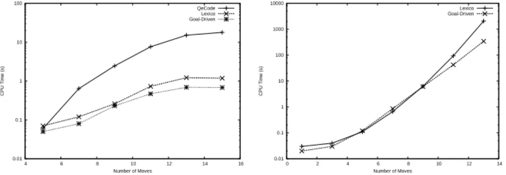
At first we tried our solver on 4×4 grids, with alignments of 3 pieces. We ran QeCode and our solver with Lexicographical heuristic (Lexico) or with Goal-Driven heuristic on problems with different number of allowed moves, from 5 to 15. We compare the time taken to solve instances.
The results are presented in Figure 1 (note the log scale). There is a solution for 9 allowed moves and more. As we can see, our solver with lexicographical value ordering solves these instances faster than QeCode. It can be explained by different ways. First, it is possible that Choco works faster in propagating constraints defined as we did. The second reason is that QeCode uses cascade propagation (propagation on the whole problem for each instantiation), whereas
our solver propagates only the rules of the current scope. Thus, our solver spends less time in propagation. We can see that the Goal-Driven heuristic speed up the resolution. It is about twice as fast as with Lexico.
0.01 0.1 1 10 100 4 6 8 10 12 14 16 CPU Time (s) Number of Moves QeCode Lexico Goal-Driven
Fig. 1.Connect-3, on 4x4 grid
0.01 0.1 1 10 100 1000 10000 0 2 4 6 8 10 12 14 CPU Time (s) Number of Moves Lexico Goal-Driven
Fig. 2.Connect-4, on 7x6 grid
In next experiments, we only compare our solver with Lexicographical value ordering and with Goal-Driven value ordering because QeCode was significantly slower and the aim is to test the accuracy of our heuristic.
In Figure 2, the real Connect-4 game is solved. We vary the number of moves from 1 to 13 and compare the performance in terms of running time. For a number of moves less than 9, Goal-Driven heuristic does not improve the per-formance, but from this point, the heuristic seems to be useful. In this problem, all instances we tested are unsatisfiable.
0.01 0.1 1 10 100 1000 10000 100000 0 2 4 6 8 10 12 14 16 18 CPU Time (s) Number of Moves Lexico Goal-Driven
Fig. 3.Noughts and Crosses, on 5x5 grid
In Figure 3, we solve the game of Noughts and Crosses. This is the same problem except the gravity constraint which does not exist in this game. It
is possible to put a piece on any free cell in the board. Instead of having n choices for a move, we have n×m choices. In the problem we tested, the aim is to align 3 pieces. This problem has a solution for 5 moves. We see that the Goal-Driven heuristic is very efficient here for solvable problems. Adding allowed moves (increasing the depth of analysis) has not a big influence on the running time of our solver with the Goal-Driven heuristic. The heuristic seems to be efficient when there are more allowed moves than necessary to finish the game. Discussion. More generally, when can we expect our Goal-Driven heuristic to work well? As it is based on information computed by AC, it is expected to work well on constraints that propagate a lot, i.e., tight constraints. Furthermore, as it actively uses quantifier alternation and tries to provoke wins/losses before the end of the sequence, it is expected to work well in problems where there exist winning/losing strategies that do not need to reach the end of the sequence.
7
Conclusion
In QCSP+, we cannot propagate constraints from the right of the sequence to
the left. Thus, current QCSP+ solvers propagate only from left to right. In
this paper, we have analyzed the effect of propagation from right to left. We have derived a value ordering heuristic based on this analysis. We proposed an algorithm implementing this heuristic. Our experimental results on board games show the effectiveness of the approach.
References
1. C. Ans´otegui, C. Gomes, and B. Selman. The Achille’s heel of QBF. In Proceedings AAAI’05, 2005.
2. M. Benedetti, A. Lallouet, and J. Vautard. QCSP made practical by virtue of restricted quantification. In Proceedings of IJCAI’07, pages 38–43, 2007.
3. C. Bessiere and G. Verger. Strategic constraint satisfaction problems. In Proceedings CP’06 Workshop on Modelling and Reformulation, pages 17,29, 2006.
4. L. Bordeaux and E. Montfroy. Beyond NP: Arc-consistency for quantified con-straints. In Proceedings CP’02, pages 371–386, 2002.
5. Choco. Java constraint library, http://choco.sourceforge.net/.
6. P.A. Geelen. Dual viewpoint heuristics for binary constraint satisfaction problems. In Proceedings ECAI’92, pages 31–35, 1992.
7. I.P. Gent, P. Nightingale, A. Rowley, and K. Stergiou. Solving quantified constraint satisfaction problems. Artif. Intell., 172(6-7):738–771, 2008.
8. N. Mamoulis and K. Stergiou. Algorithms for quantified constraint satisfaction problems. In Proceedings CP’04, pages 752–756, 2004.