A New procedure for evaluating the time domain boundary influence matrix of unbounded media

(1)

Publisher’s version / Version de l'éditeur:

Computers and Structures, 34, 6, pp. 843-853, 1990

READ THESE TERMS AND CONDITIONS CAREFULLY BEFORE USING THIS WEBSITE. https://nrc-publications.canada.ca/eng/copyright

Vous avez des questions? Nous pouvons vous aider. Pour communiquer directement avec un auteur, consultez la première page de la revue dans laquelle son article a été publié afin de trouver ses coordonnées. Si vous n’arrivez pas à les repérer, communiquez avec nous à PublicationsArchive-ArchivesPublications@nrc-cnrc.gc.ca.

Questions? Contact the NRC Publications Archive team at

PublicationsArchive-ArchivesPublications@nrc-cnrc.gc.ca. If you wish to email the authors directly, please see the first page of the publication for their contact information.

NRC Publications Archive

Archives des publications du CNRC

This publication could be one of several versions: author’s original, accepted manuscript or the publisher’s version. / La version de cette publication peut être l’une des suivantes : la version prépublication de l’auteur, la version acceptée du manuscrit ou la version de l’éditeur.

Access and use of this website and the material on it are subject to the Terms and Conditions set forth at

A New procedure for evaluating the time domain boundary influence

matrix of unbounded media

Hunaidi, O.

https://publications-cnrc.canada.ca/fra/droits

L’accès à ce site Web et l’utilisation de son contenu sont assujettis aux conditions présentées dans le site LISEZ CES CONDITIONS ATTENTIVEMENT AVANT D’UTILISER CE SITE WEB.

NRC Publications Record / Notice d'Archives des publications de CNRC:

https://nrc-publications.canada.ca/eng/view/object/?id=396d0639-fe52-401f-84f4-33d388057a9d https://publications-cnrc.canada.ca/fra/voir/objet/?id=396d0639-fe52-401f-84f4-33d388057a9d

(2)

Se

r

THI

Fl

2

1 d

,

no,1656

c.2

National Research Conseil national

*

Council Canada de recherches Canada

Institute for lnstitut de

Research in recherche en

Construction construction

A New Procedure for Evaluating theTime

Domain Boundary Influence Matrix of

Unbounded Media

by M.O. Al-Hunaidi

Reprinted from

Computers & Structures Vol. 34, No. 6

1990

p. 843-853

(IRC Paper No. 1656)

(3)

La methode des elements finis ne peut s'appliquer qu'aux domaines finis comportant des limites bien definies. Dans le cas des problemes dynamiques mettant en cause des milieux non bombs, les limites du modele fini, si elles restent non trait&, donnent une fausse idee du comportement physique reel du problbme. Pour bien des problemes, il est possible de formuler les conditions de limites dites muettes, qui reproduisent parfaitement l'effet du milieu non born6 tronque. Malheureusement, la plupart de ces conditions sont formul&s correctement dans le domaine frequentiel.

Ce document fait etat d'une nouvelle procedure qui permet d'utiliser ces conditions de limites dependant de la frequence pour calculer la matrice d'influence, dans le domaine temporel, du milieu non bomb tronqub. Cette matrice, qui a ete deaite dans un document publik plus t6t, sert B calculer la reponse sans reflexion de la limite de troncation une phase de temps avant la position presente dans le temps. La reponse connue de la limite sert alors de condition prescrite pour le modele fini. Afin de determiner l'efficacitk de la nouvelle procedure, l'auteur presente un exemple unidimensionnel comportant une condition de limite dependant de la frequence. I1 examine aussi deux autres conditions de limites muettes formulees directement dans le domaine temporel.

(4)

Computers & Structures Vol. 34, No. 6, pp. 843-853, 1990

Printed in Great Britain.

0045-7949190 $3.00

+

0.00

Pergamon Press plc

A NEW PROCEDURE FOR EVALUATING THE TIME

DOMAIN BOUNDARY INFLUENCE MATRIX OF

UNBOUNDED MEDIA

M. 0. AL-HUNAIDI

Institute for Research in Construction, National Research Council of Canada, Ottawa, Ontario, Canada KIA OR6

(Received 15 January 1989)

Abstract-The finite element method can only deal with finite domains with well defined boundaries. For dynamic problems involving unbounded media, the boundaries of the finite model distort the real physical behaviour of the problem if they remain untreated. For many problems it is possible to formulate so-called silent boundary conditions which perfectly simulate the effect of the truncated unbounded medium. Unfortunately, most of these conditions are properly formulated in the frequency domain.

The present paper introduces a new procedure which employs these frequency-dependent boundary conditions to calculate the time domain influence matrix of the truncated unbounded medium. This matrix, which was introduced in a previous publication, is used to calculate the reflection-free response of the truncation boundary one time step ahead of the present time station. The known boundary response is then used as a prescribed condition for the finite model. A one-dimensional example with a frequency-dependent boundary condition is presented to examine the effectiveness of the new procedure. Two other silent boundary conditions formulated directly in the time domain are also examined.

1. INTRODUCTION

In the numerical analysis of wave propagation problems in unbounded media, it is customary to employ silent boundary conditions at the truncation edges of the finite model. The purpose of these boundary conditions is to simulate the effect of the truncated domain and hence preserve the real physical behaviour of the problem.

Silent boundaries are generally classified into two categories: (i) local boundaries and (ii) nonlocal boundaries. Local silent boundaries, as the name implies, do not introduce boundary node coupling other than that imposed by the spatial and temporal discretizations employed. The boundary nodes

4

employ information from neighbouring points only at the current or a few previous time stations. These boundaries are frequency-independent and therefore 1

I can be utilized directly in time domain analyses. They are, however, imperfect absorbers because they are based on physical or mathematical approximations. Nonlocal silent boundaries, on the other hand, are perfect absorbers. Unfortunately, they are properly formulated in the frequency domain and they couple all degrees of freedom on the boundary-hence the name nonlocal boundaries. The radiation condition of the truncated infinite domain is represented by means of a frequency-dependent dynamic stiffness matrix which relates the nodal displacements and nodal forces at the truncation boundary. This matrix is based on analytical or semi-analytical solutions of the equation of motion in the infinite medium, and it can be conveniently calculated using the boundary element method [I].

The well known consistent boundaries of [2,3] are examples of nonlocal boundaries. These are devel- oped for layered soil sites resting on a rigid base under plane strain or axisymmetric conditions. The dynamic stiffness matrix of the boundary is obtained by employing horizontal displacement functions corresponding to the anaIytica1 solution of the equation of motion and vertical displacement functions consistent with the finite element discretization of the interior region (four-node bilinear elements were employed). The wave numbers of all waves that can propagate in the layered medium are determined for the frequency under consideration. Hence, proper absorption of all waves is achieved. The only approx- imation introduced is that due to using displacement functions consistent with those of the finite element discretization in the vertical direction.

Nonlocal silent boundaries can be conveniently and efficiently applied in linear analyses performed in the frequency domain. Transient loading can be handled by the Fourier transform method and the procedures to do so are well established [4]. For nonlinear analysis, however, solution in the frequency domain is not possible, unless so-called equivalent linearization techniques are employed.

True nonlinear analyses should be performed directly in the time domain, i.e. using step-by-step time integration methods. With the rapid advancement of truly nonlinear time domain analysis methods, there is an increasing demand for developing and imple- menting high quality silent boundaries that can be used in conjunction with these methods.

This paper advances the concept of a previously silent boundary based on the so-called time domain

(5)

BOUNDARY 0

BOUNDARY I .

Fig. 1. Substructuring of the soil-structure system for the TDBIM approach.

boundary influence matrix (TDBIM) [5]. In this silent boundary approach, TDBIM stores the response of boundary degrees of freedom due to unit triangular nodal forces at degrees of freedom coupled to the boundary. TDBIM is then used to calculate the boundary response one time step ahead of the last calculated time station, which in turn is used to calculate the dynamic stiffness contribution of the truncated infinite part.

In the previous approach [S], TDBIM was calculated directly in the time domain using an extensive finite element mesh. Therefore computational savings that may be gained by employing this approach are limited to situations in which many analyses of the same problem are to be performed. This procedure will subsequently be referred to as the 'direct approach' or as 'direct calculations'.

In the present paper the TDBIM is calculated indirectly in the frequency domain in which the highly accurate nonlocal silent boundaries can be properly formulated. This eliminates the need for an extensive mesh and hence leads to a more economical TDBIM

approach. This procedure will subsequently be referred to as the 'indirect approach' or as 'indirect

calculations'. _I

Section 2 of this paper summarizes the TDBIM

₅

_! approach. Section 3 presents the new advancement

.

using indirect calculations in the frequency domain.

i

The fourth section presents an example to demon-

strate that the high accuracy of the original TDBIM

:

1

approach is preserved with the new procedure.

2. THE TIME DOMAIN BOUNDARY INFLUENCE MATRIX

APPROACH

I

In this section, the silent boundary based on the direct TDBIM approach [5] is reviewed by considering the soil-structure model shown in Fig. la. This model is substructured into three parts: (i) structure, (ii) soil and (iii) interface zone, as shown in Fig. lb. The structure part consists of the structure itself and a portion of the supporting soil which may be

nonlinear and/or geometrically irregular. The soil part is assumed to be linearly elastic (or linearly

(6)

Time domain boundary influence matrix of unbounded media 845

viscoelastic). The interface zone consists of one strip of elements which are considered as four-noded for simplicity of presentation. These elements separate the structure and the soil parts. Consequently they contain all degrees of freedom coupled by the stiffness matrix to degrees of freedom on the boundary B of the soil part. The mass matrix of the interface zone is assumed to be diagonal.

The finite element equations of the soil part and interface zone combined may be written in the follow-

C

ing form:

a time domain boundary influence matrix [Dl is calculated. This matrix stores the response of boundary B degrees of freedom due to unit triangular pulse forms at degrees of freedom of boundary I. An

element (i, j, k) of the matrix is the respom of degree of freedom i of boundary B at time step k due to unit triangular pulse force at degree of Fmdom j of boundary I. Matrix [Dl is calculated by solving eqn (1) for unit triangular pulse forces, two time steps long, applied at degrees of freedom of boundary I,

one at a time. The finite element mesh of the soil part

should be large enough such that no reflections at its

far boundary may reach the boundary B while the solution is in progress.

In order to calculate the response { u b ) of the boundary B, the internal attending nodal forces

{ A )

are imagined to be represented by triangular pulses,

as shown in Fig. 2. If an explicit time integration

scheme is used (at least for the interface zone], a

In the above equation the m and k matrices are

submatrices of the mass and stiffness matrices of the FORCE

soil and interface zone substructures. The matrix partitioning can be directly understood with reference to Fig. lb. {ti} and { u } are nodal accelerations and displacements, respectively. j; in the above equation andfi in Fig. l b are the attending internal nodal force

vectors acting on boundary I between the structure

1

0 At 2At 3At 4At 5At Bdt 7At

and the interface zone. These forces are of equal

magnitude but have opposite directions.

II

Similarly, the equations of motion of the finite

model consisting of the structure part and the inter- I I I I 1 I

face zone combined are

m,

+

m,,

where {'P,} and { ' P i } are internal nodal forces result-

t

I

f ing from the discretized nonlinear constitutive rela- tionships of the structure paFt.

They

may depend on the displacements (u,) and { u , ) and the velocities {ti,)

1

and ( t i , ] and their time histories.

For

the sake of

simplicity, the structure is assumed to be linearly

elastic. Hence eqn (2) becomes

In eqns (2) and (3), it is assumed that the response

+

of the boundary B, {u,}, is known in advance and therefore it is treated as a prescribed condition by transferring the contribution {kibub} to the right-hand

side of the equilibrium equations. Fig. 2. Representation of forcetime history as a summa-

(7)

nonzero displacement response at any of the degrees of freedom on boundary B due to a triangular pulse force, say over time steps m and m

+

1, will only start at the end of time step m

+

1 or later. This can be seen from eqns (4)-(8) of the explicit algorithm, explained further on in this section. Therefore, it is possible to calculate a reflection-free boundary response tub} one time step ahead of the present time station using the nodal force vector

{ A }

at the end of the present and past time stations.

The explicit predictor-corrector algorithm based on Newmark's family of methods [6, 71 is used for the solution of the equations of motion [M]{ii(t))

+

[C]{u(t))

+

[K]{u(t)} = {F(t)). In this algorithm, the equations of motion at time t +At are satisfied with the following predictors for the displacement and velocity vectors:

and

where a tilde is used to designate predictor values. y and

B

are free parameters which control the stability and accuracy of the algorithm. Substituting the above predictor values in the equations of motion at time t

+

At, the accelerations are solved as follows:

No inversion is performed as the mass matrix is diagonalized. The displacement and velocity vectors are then corrected as follows:

and

of degree of freedom i at the end of time step ISTEP

+

1 is given by

LFNEQ ISTEP

ui = F ( j , k) x D(i, j, ISTEP - K

+

2) (9)

j = l k = l

where F ( j , k) is the attending nodal force at degree I of freedom j on boundary I at the end of time step k.

LFNEQ is the total number of degrees of freedom on boundary I. A convenient local numbering procedure

for nodes of boundaries I and B is presented in [5].

A

3. INDIRECT TDBIM CALCULATION

I The cost of calculating the time domain boundary

influence matrix directly in the time domain using an extended mesh is admittedly substantial. Computa- tional gains are only possible for situations in which many analyses of the same problem are required. The reason an extended mesh is required for the TDBIM direct approach is to ensure a reflection-free boundary response. Consequently, analyses which are performed using TDBIM calculated directly are exact in the numerical sense for the spatial and temporal discretizations employed [S].

An alternative and more economical procedure for calculating a reflection-free TDBIM is introduced in this section. The procedure eliminates the need for an extended mesh and therefore drastically reduces the computational burden of the direct approach. In this procedure, TDBIM is indirectly calculated in the frequency domain in which the highly accurate nonlocal silent boundaries can be properly formulated. Except for this alteration, the silent boundary based on the TDBIM approach remains unchanged.

The time variable is eliminated by expressing the input in the form of a Fourier series, i.e. as a sum of harmonics. The response to each term of the series is simply the response to a harmonic input. By the principle of superposition, the total response is the sum of the responses to all terms in the series. For a periodic real function of period T p , the Fourier series in exponential form is

The above explanation also applies to the nodal CO

P(t ) = Re

1

c, exp(io, t) interaction forces at boundary B, calculated using the

["=.

predictor values of displacement and velocity.

Therefore, instead of calculating and prescribing the where boundary response {ub}, one may alternatively calcu-

late and prescribe the nodal interaction forces {&). _{n = O} The interaction forces

if/}

and {f,) acting on

boundary B (see Fig. lb) are of equal magnitude but

have opposite directions. P(t) exp(-iw,t) dt, n = l,2,3,

.

The boundary response {ub} is simply the superpo- (1 1) sition of the results of multiplying the amplitudes of

triangular pulses representing the time history of the

attending nodal force

{ A }

by the corresponding (12) influence coefficients of the boundary influence

(8)

Time domain boundary influence matrix of unbounded media

FORCE

A

I

b

Fig. 3. Periodic pulse function.

)

Evaluating eqn (I I) for the function (see Fig. 3) In this case the solution is performed for few frequen- _{cies, then the response at the intermediate frequencies}

1 is obtained by interpolation. This aspect will be

if O < t < A t _{considered in a future publication.}

The representation of internal nodal forces as a if A t < t < 2 A t (14) sum of triangular pulses (see Fig. 2) implies the assumption of linear variation of these forces within if 2 A t < t _{each time step At. This assumption is of no conse-} quence on the TDBIM direct calculation procedure

yields _{because step-by-step integration schemes satisfy equi-}

librium only at discrete time points At apart. This is At

co = - (15) not so for solutions performed in the frequency

T~ domain. However, numerical results obtained with

8 the proposed TDBIM indirect calculation procedure

c, =

-

_Tp_Atwlsin2(io, At) exp(i4,) (16) (see Sec. 4.2) indicate that the assumption of linear variation of internal nodal forces is reasonable. where the phase angle

4,

is given by 4. EXAMPLE: SEMI-INFINITE ROD

4" = -Atw,. (1 7) 4.1. TDBZM calculation

The new indirect TDBIM calculation procedure is The period Tp should be long enough to allow the examined by considering the one-dimensional case of material and radiation damping of the system enough an undamped semi-infinite rod with an exponentially time to attenuate the response due to one pulse before increasing area, shown in Fig. 4. The cross-sectional the beginning of the next pulse. This requirement area is equal to

introduces no practical difficulty because the damp-

ing of soils is high and hence the period Tp does not A (2 = A0 ~ X P ( Z

If)

(19) have to be very long. The higher the damping, the

shorter the period Tp that need be used. A small where A, is the area at z = 0 and f is a constant.

rn _{period Tp leads to a small number of frequency that} _{For this simple case, the TDBIM is a single element}

is of interest in the Fourier series, and hence reduces + matrix which will simply be referred to as the influ-

the computational effort of calculating TDBIM, as ence coefficient. Analytical solutions of this case have

1

will be explained next. been derived in [l]. These solutions are used in this The highest frequency of interest, om,, , in the section for the indirect calculation of the time domain Fourier series need not exceed the cut-off frequency, boundary influence coefficient as suggested in Sec. 3. w,,,, of finite elements used for space discretization. For harmonic excitation with frequency a , the The number of Fourier series terms, NI, that need be equation of motion of a rod with a varying cross- considered is then given by sectional area A is

Fourier series terms with frequencies above the cut- where C, is the longitudinal wave velocity defined as

off frequency are simply neglected. From eqn (181, it

can be seen that the shorter T,, the smaller the number

of frequencies, N,, which need be considered. The .I =

J,

(21)

computational effort may be further reduced by

(9)

\ / BOUNDARY I \

&

,BOUNDARY ,B

Fig. 4. Semi-infinite rod with exponentially increasing cross-sectional area.

material density. Defining the dimensionless fre- in the negative z-direction. In order to satisfy the quency 6 as radiation condition of a semi-infinite rod, the second term should be discarded. Therefore setting b equal

-

Wf

m = - to zero, the displacement amplitudes at boundaries I

CI (22) and B in Fig. 4 are equal to

and substituting eqn (19) into eqn (20) yields

wI = a exp(-

$)

exp(

-

ikz,) (27)

1 G2

w,+-w,+-w

=o.

f

(23) _wB₌_{a exp(-}

$1

_{exp(- ikzB).}

(28) The solution of the above equation is found to be [I]

Eliminating a from eqn (27) leads to w(G) = a exp

(

--

2

exp(-ikz)

wI = exp

(

d )WB (29)

where the depth of the interface zone dis equal to where a and b are integration constants, and k is the

wave number defined as

The corresponding internal force

P,

acting on (25) boundary I of the interface zone is given by with the phase velocity c given by _P.₌

_-

_FA._{r x n l}

(31) (26) Evaluating

W,~I,.

,, yields

For frequencies 6

<

0.5 the wave number k is

P~

= ;K(I

+

, / w ) w l (32) purely imaginary, therefore motion does not propa-

gate but diminishes exponentially along the z-axis. where K is the static stiffness coefficient given by For higher frequencies, the first term of eqn (24)

represents a wave propagating in the positive z-direc- _{K =}EAo exp(z,lf)

f

(10)

Time domain boundary influence matrix of unbounded media 849

Finally, substituting eqn (29) into (32), the relation- tion force Po(?) defined as ship between the internal force PI acting on boundary

I, and the displacement w , of boundary B is PO = p ~ , ( t ) / ( K w o ) (42)

where K is the static stiffness coefficient of the infinite

P~ = W E (34) rod. From eqn (33),

where K = EA,/f: (43)

S I B ( G ) = K(1

+

.,/-I

Finite one-dimensional elements of equal length

Az = 0.1 f a r e used for spatial discretization of the

b

rod. Displacement variation within each element is

x exp

( )

(35) assumed to be linear. A diagonal mass matrix is

5

Hence employed. ming the corresponding row of the consistent mass Diagonal elements are computed by sum- matrix as follows:

where the influence coefficient DIB(G) is given by

By the principle of superposition, the time domain boundary influence coefficient D,(t) is the summa- tion of the responses to all terms in the Fourier series expression of the periodic triangular pulse in Fig. 3. Therefore

where c,, are Fourier series coefficients defined by eqn (1 1); 5 , is given by

4.2. Numerical veriJication

The accuracy of the proposed TDBIM indirect calculation procedure is numerically examined using the semi-infinite rod with exponentially increasing area introduced in the previous section. For compari- son the popular standard viscous boundary [9] and the direct energy deletion boundary [ l o ] , which are of the local type, are also examined.

*

A longitudinal wave field is generated in the rod by a displacement controlled transient loading applied at the top end. The input has the form

The semi-infinite part of the rod is truncated at distance 5 Az where the silent boundary is placed. The predictor-corrector algorithm based on Newmark's family of methods, explained in Sec. 2, is used for time integration with parameters y = 0.5 and

fl

= 0 .

The size of the time step Aiis selected equal to 0.099 for all calculations except for the standard viscous boundary where it is selected equal to 0.05 for numerical stability.

The duration of the input pulse

6

is selected equal to 5. The Fourier spectrum of the pulse with this duration obtained from the equation

is presented in Fig. 5. It can be seen that the frequency content covers a wide range that includes the cut-off frequency fi = 0.5 of the rod.

Results of the silent boundary are compared with the results obtained using an extended finite element mesh, i.e, a very large mesh in which no reflections reach the top end of the rod. Results of the extended mesh are referred to as the reference solution.

First, the silent boundary based on the TDBIM indirect approach is considered. The preliminary step in this approach is to determine the number of Fourier series terms,

Nf,

that should be considered. The cut-off frequency of the finite elements used is assumed to be equal to that of one-dimensional elements of a prismatic rod. For a diagonal mass matrix formulation, this frequency is given by [8]

where

7

is dimensionless time defined as

where Az is the element size. From eqn (18), the

i =

tc,lf. (41) , number of Fourier series terms NJ that need be

considered is given by The reaction force Po(?) is calculated at the top end

of the rod. Performance of the silent boundary is Tp C I

Nf<

-

(11)

Fig. 5. Fourier spectrum of the, input pulse.

Substituting Az = 0.1 f and defining the dimensionless period

Tp

as

yields

Figure 6 presents the time domain boundary influ- ence coefficient D,,(i) calculated by eqri (38) with

Tp

and

Nf

chosen equal to 300 At and 95, respectively. This is an appropriate choice as the response to one pulse is almost fully attenuated before the beginning of the next pulse. Hence, the response due to a single pulse of the periodic function of finite period

T'

is practically equivalent to the nonzero response due to periodic pulse function with

Tp+

co. The performance of the TDBIM indirect approach is excellent as can be seen from comparison with the reference solution in Fig. 7.

The number of frequencies N/ considered in this

example is calculated by eqn (49). By using a smaller number of frequencies for the same period

Fp,

numerical instability was observed in the calculated response. On the other hand, using a number of frequencies greater than that calculated by eqn (49) yields almost the same response as that in Fig. 7 and therefore is a waste of computational effort. Expect- edly, it was also observed that using a period

Tp

shorter than that used above produces a poor response. The reason for this is that the response to one pulse may not be attenuated before the beginning of the next pulse.

For the standard viscous boundary, the radiation condition is simulated by applying a boundary trac- tion a, given by

a,= - p ~ , ~ ~ (50)

where a dot denotes time derivative. The corresponding boundary force is defined as

9

0

I

-40 -30 -20 -10 0 10 20 30 40

DIMENSIONLESS TIME

r=

tcl/f

(12)

Time domain boundary influence matrix of unbounded media 0 r. n 1, u! -00 la

8 8 2

Z

8

52

E ' I

z 1

1 0 5 10 15 20 25 30 35 40 45 50 DIMENSIONLESS TlME

f

= t$/f

Fig. 7. Reaction force response employing the TDBIM approach.

The performance of the viscous boundary is disappointing as can be seen from comparison with the reference solution in Fig. 8. This poor performance is easily explained. The boundary condition given by eqn (51) is the exact radiation condition of a semi- infinite prismatic rod, i.e. the case off +co, as can be seen from eqn (32). Therefore, this boundary condi- tion represents a physical situation in which the truncated part of the rod with exponentially increasing area is replaced by a semi-infinite prismatic rod of cross-sectional area equal to A,exp(Z,/f), as illustrated in Fig. 9.

In the direct energy deletion silent boundary [lo], the wave absorption mechanism is based on directly deleting wave energy in a small extended boundary region so that the front of reflected waves is continu- ally held from the interior region of interest. The wave field continuity across the boundary is preserved by a special numerical scheme in which a separate solution for the extended boundary region is performed in parallel with the solution of the complete model.

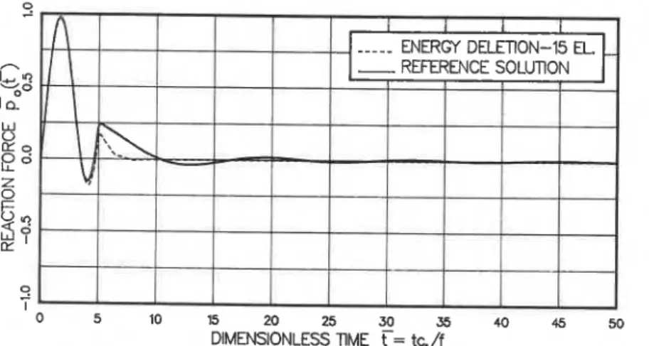
Results of this boundary obtained with a five- element extended boundary region are presented in

Fig. 10. The results are not as disappointing as those of the standard viscous boundary. Improvement of the performance of this boundary can be achieved by increasing the size of the extended boundary region[lO]. Figure 11 presents satisfactory results obtained with a 15-element extended boundary region.

5. SUMMARY

The silent boundary concept based on the time domain boundary influence matrix (TDBIM) [S] is advanced and refined by means of an alternative calculation procedure. In the new procedure, the TDBIM is indirectly calculated in the frequency domain in which perfectly absorbing nonlocal boundaries can be properly formulated. Employing nonlocal silent boundaries eliminates the need for an extended mesh and hence reduces the computational burden of the original calculation procedure.

The unit triangular pulse force used as input in TDBIM calculations is expressed in the form of a Fourier series. The number of Fourier frequencies considered need not exceed the cut-off frequency of the finite elements employed.

5

0 5 10 15 20 25 35

DIMENSIONLESS TlME

?=

t$/f

(13)

V VISCOUS

DAMPER:

Fig. 9. Physical interpretation of the viscous boundary condition.

9

-

_I

0 5 10 15 20 25 30 35 40 45 50

DIMENSIONLESS TIME

f =

tc,/f

fig. 10. Reaction force response employing the direct energy deletion boundary with a five-element boundary zone. 9

-

n 1 1 0

4"

la

Y

;z

Z

E

$ 7

Ix 9

-

_I 0 5 10 15 20 25 30 35 40 45 50 DIMENSIONLESS TlME

f

= t%/f

Fig. 1 1 . Reaction force response employing the direct energy deletion boundary with a 15-element boundary zone.

(14)

Time domain boundary influence matrix of unbounded media 853 The new indirect calculation procedure is applied 4. J. Lysmer, T. Udaka, C.-F. Tsai and H. B. Seed, to the case of a semi-infinite rod with exponentially FLUSH: a computer Program for approximate 3-D analysis of soil-structure interaction problems. Report increasing cross-sectional area in which the radiation _No._{EERC 75-30, Earthquake Engineering Research} condition is frequency-dependent. Comparison of the Center, University of California, Berkeley, California numerical results with those obtained with an ex- (1975).

tended finite element mesh is very satisfactory. 5. M. 0. Al-Hunaidi, Analysis of wave propagation in unbounded media. C o m ~ u t . Struct. 33.1037-1045 (1989). Acknowledgements-The author wishes to express his ap-

preciation to J. H. Rainer for his many helpful comments. This paper is a contribution of the Institute for Research in

t

Construction, National Research Council of Canada.

REFERENCES

b

1. J. P. Wolf, Dynamic Soil-Structure Interacrion, pp. 114123. Prentice-Hall, Englewood Cliffs, NJ (1985).

2. G. Waas, Earth vibration effects and abatement for military facilities. Technical Report S-71-14, U.S. Army Engineer Waterways Experiment Station, Vicksburg, Mississippi (1972).

3. J. Lysmer and G. Waas, Shear waves in plane infinite structure. ASCE J. Engng Mech. Div. 98,85-105 (1972).

6. T. J. R. Hughes and W. K. Liu, Implicit-explicit finite elements in transient analyses: stability theory. J. appl.

Mech. 45, 371-374 (1978).

7. T. J. R. Hughes and W. K. Liu, Implicit-explicit finite elements in transient analyses: implementation and numerical examples. J. appl. Mech. 45, 375-378 (1978). 8. T. Belytschko, An overview of semidiscretization and

time integration procedures. In Computational Methods for Transient Analysis (Edited by T. Belytschko and T. J. R. Hughes), pp. 2 4 5 . Elsevier, New York (1983). 9. J. Lysmer and R. L. Kuhlemeyer, Finite dynamic model for infinite media. ASCE J. Engng Mech. Div. 95,

859377 (1969).

10. M. 0. Al-Hunaidi, I. Towhata and K. Ishihara, Silent boundary for time domain wave motion analyses based on direct energy deletion approach. Int. J. Soil Dynam.