Cell Polarity: Focal Adhesion and Actin Dynamics in Migrating Cells

(1)

HAL Id: hal-02910995

https://hal.archives-ouvertes.fr/hal-02910995

Submitted on 3 Aug 2020

HAL is a multi-disciplinary open access

archive for the deposit and dissemination of

sci-entific research documents, whether they are

pub-lished or not. The documents may come from

teaching and research institutions in France or

abroad, or from public or private research centers.

L’archive ouverte pluridisciplinaire HAL, est

destinée au dépôt et à la diffusion de documents

scientifiques de niveau recherche, publiés ou non,

émanant des établissements d’enseignement et de

recherche français ou étrangers, des laboratoires

publics ou privés.

Cell Polarity: Focal Adhesion and Actin Dynamics in

Migrating Cells

Perrine Paul-Gilloteaux, Christoph Möhl

To cite this version:

Perrine Paul-Gilloteaux, Christoph Möhl. Cell Polarity: Focal Adhesion and Actin Dynamics in

Migrating Cells. Kota Miura. Bioimage Data Analysis, Wiley-VCH, pp.198-218, 2016,

978-3-527-80092-6. �hal-02910995�

(2)

8 Cell Polarity: Focal Adhesion and Actin Dynamics in

Migrating Cells

Perrine Pau/-Gilloteaux7

'2 and Christoph Möhf 1 _{Institut Curie, Centre de Recherche, Paris 75248, France} 2

Cell and Tissue Imaging Facility, PICT-IBiSA, CNRS, UMR 144, Paris 75248, France 3

German Center of Neurodegenerative Diseases (DZNE), Image and Data Analysis Facility (IDAF), Core Facilities, Hofbeinstraße 13-15, 53175 Bonn, Germany

8.1 Aim

In this chapter, we learn to identify image objects in time-lapse movies of single migrating cells. We analyze their shape, growth dynamics, and movement of the associated actin network, which is recorded in a separate channel. This way, we get familiar with optical flow analysis and learn how to integrate the information of different image data sources to discover relationships between different object features.

8.2 Introduction

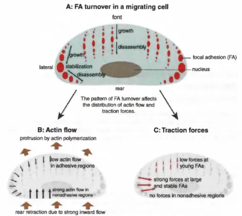
Effective locomotion of migrating cells depends on the coordinated interplay between protrusive, contractile, and adhesive components of the cytoskeleton and the plasma membrane. Traction forces are generated by a viscoelastic network of actin filaments interacting with myosin II motors. These forces are applied to the substrate through distinct focal adhesions (FAs). These are protein clusters at the cell plasma membrane coupling actin filaments to extracellular matrix proteins.

Forward movement is enabled by polarized growth dynamics of F As (see Figure 8.1): At the cell front, new FAs are assembled, while FA disassembly mainly occurs at the cell's rear and center. The coupling of actin to FAs, and hence the transduction of tractile forces to the substrate, may also vary between different types of F As. This coupling can be measured indirectly by the movement of actin above F As. While tight coupling is indicated by slow actin flow

(3)

A: FA turn over in a migrating cell font •• ; • !growth •

.~

.

•._ I 4

f ♦

t t •

.. l

I ~

!

t

f

wsassemtw¡f

?

J • ••

I

rrowt~ • •

! :

·t

I,.-

focal adhesion (FA)

lateral • ~tabilization ~--- _ • _ _;

li.,

nucleus

:"l~sassem~

..

••

'

I

The pattern of FA turnover affects \ rear the distribution of actin flow and

traction forces.

B: Actin flow

protrusion by actin polymerization

.. + •

l 1:

I

~ow actin flow \ ~ in adhesive regions

~

...

/,,, f

Î

f f

strong act~ flow _in

,- nonadhesive regrons

C: Traction forces

l ¡ • low forces at

~ Í f f young FAs ~ strong forces at large

____...and stable FAs

AO forces in nonadhesive regions

+ + +

rear retraction due to strong inward flow

Figure 8.1 The interplay of focal adhesion and actin dynamics as well as resulting traction forces in a migrating cell.

due to higher friction, weak substrate coupling correlates with fast actin movement [1,2].

8.2.1

Questions to Solve

Identify F As in time-lapse movies of migrating cells and measure their size, growth rate, and the ~ctin flow above them.

• What is the relationship between growth rate, actin flow, and size?

• Do growing FAs (positive growth rate) exhibit a stronger or weaker actin coupling compared with disassembling F As (negative growth rate)?

8.2.2 Data Set

We analyze four time series with one migrating cell in each (human keratinocyte on fibronectin-coated glass substrate). The cells express the fluorescently labeled

(4)

FA protein vinculin (label: dsRed) and actin (label: GFP). Each time series con- sists of two movies recorded one after the other:

1) Red epifluorescence: 6 min time lapse of focal adhesion dynamics at low temporal frequency (2 frames/min; movies suffixed with _1, called movie 1). 2) Green TIRFl): 80 s actin dynamics at high temporal frequency {15 frames/

min; movies suffixed with _2, called movie 2).

Due to the high sampling rate for actin flow quantification, FA and actin dynamics were not recorded simultaneously.

8.2.3

Overview of Data Processing

• Step 1: Segmentation of movie 1 to identify FA objects (Fiji).

• Step 2: Quantification of actin flow above FA objects in movie 2 (Matlab). • Step 3: Calculation of features of FA objects: area, growth rate, and mean actin

flow (Matlab).

• Step 4: Statistical analysis of the relationship between FA area, growth rate, and actin flow (Matlab).

We use Fiji2> for FA segmentation and Matlab to quantify the actin flow and calculate features of the detected FA objects (from the analysis in Fiji), for statistical analysis and plotting of results. In addition to the main distribution of Matlab, we will use the image processing toolbox (for labeling operations and displaying images).

8.3

Step 1: Identification of Focal Adhesions

8.3.1

Workflow

We first develop a routine in ImageJ Macro language to segment F As over time in time-lapse movie l.

This routine should execute the following tasks:

• Import raw data in native microscopy format: movie suffixed _1 in zvi format.

{1_1.zvi, 2_1.zvi, 3_1.zvi, 4_1.zvi)

l} Total internal reflection microscopy: A method to image only fluorescent signals in close proxim- ity to the cover slip. It is used here to image actin flow only in regions of cell adhesion, where the cell membrane is adjacent to the glass. Another advantage is the exclusion of cytoplasmic background signal.

(5)

Input Output

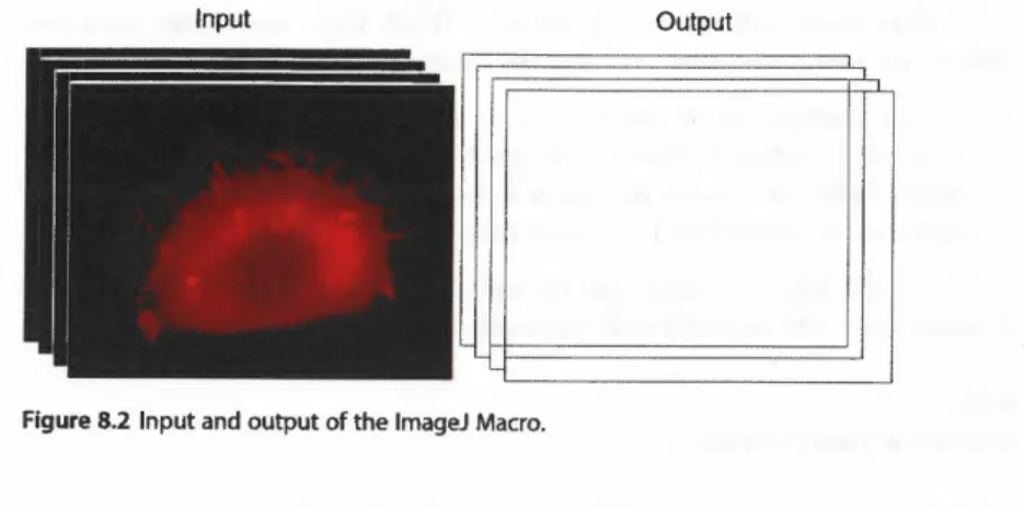
Figure 8.2 Input and output of the lmageJ Macro.

• Automated detection of FA regíons.A black and white mask image of the seg- mented objects is created for each frame.

• Data export: The masks are exported in TIF format (see Figure 8.2): The TIF stacks can later be imported in Matlab for feature processing and integration with the actin flow data.

To automate the processing of the image time series, we write a script in ImageJ Macro language by recording the individual steps.

1) Open the recorder with [Plugins >Macros> Record ... ] .

2) Use the LOCI importer to load image data in zvi format [Plugins >LOCI> Bio-Formats Importer].

3) If you have a look through the whole time series, you will notice that the sample bleaches out over time. Since we want to detect FA objects by an intensity threshold, we have to correct for the bleaching. Otherwise, the objects tend to be smaller (as they become darker) toward the end of the movie. We correct for bleaching by applying [Image> Adjust > Bleach Correction]. You can choose several options for bleach correction. By visual inspection, it turns out that the "histogram matching" method works best. Here, the shape of the gray value distribution for each frame is adapted to the first frame. 3

>

4) Smooth raw images with a Gaussian filter over

x,

y, and time [Process> Filters >Gaussian Blur 3D ... ] The smoothing removes the image noise and will result in smoother outlines of the F As we want to detect later. Sigma corresponds to the radius of the filter window. Here the third dimension is the time, but it is called z in the command. Suggested parameters for sigma are x

=

4, y

=

4, and z

=

6.

3) More information about the different bleaching correction methods implemented in Fiji can be found at fiji.sc/Bleach_Correction.

(6)

5) As images were collected in epifluorescence, cytoplasmic background signal is very strong." We remove the background by applying the "Subtract Background" function [Process > Subtract Background ... J. This function executes two steps: It first applies a large average filter, resulting in a strongly blurred image. If the filter window is significantly larger than the objects of interest, the blurred image is a good approximation of the cytoplasmic background (suggested value for the radius is 17). In the second step, this background image is subtracted from the original image resulting in the background corrected image. The resulting stack will be referred to as "corrlm".

1 //bleach correction

2 run { "Bleach Correction", "correction= [Histogram Matching] 11 ) ;

3 corrim=getimageID{);

4 //filtering+++++++++++++++++++++++++++++++++++++++++++++ 5 //smooth with gaaussian

6 run ( "Gaussian Blur 3D ... 11_,_{"x=4 y=4}_{z=6") ;}

7 //subtract background 8 run { "Subtract Background ... 11

, "rolling=l 7 stack");

9 run {"Enhance Contrast11

,11saturated=O.l11);

code/Step 1 _FA_segmentation.ijm

6) Up to now, we corrected our time series for bleaching, noise, and cytoplasmic background and we are ready to detect FA objects by simple intensity thresholding. We can test several algorithms for calculating an automatic threshold by executing [Image > Adjust > Auto Threshold] and setting "Method" to "Try all". It will take a while to calculate all different thresholds. You can follow the progress in the log window. Finally, an image montage is displayed showing binary masks for all the different algorithms. This montage allows us to quickly pick an algorithm where the threshold is suitable. In our case, the "IsoData" method does a good job in detecting the FA objects. We run again [Image > Adjust > Auto Threshold] with the option "IsoData". We check also the options "Stack" and "Use Stack Histo- gram". With the "Stack" option checked, masks will be generated for the whole time series. The "Use Stack Histogram" option ensures that one global threshold is calculated for the whole time series, and not a new threshold for each frame. Since we corrected for bleaching in the first step, we do not have to adapt the threshold over time.

4) In epifluorescence, the optical section is not restricted in z (which is the case in confocal, light sheet, or TIRF microscopy). Due to the wide optical plane, a lot of fluorescent signals from cytoplasmic vinculin-GFP are imaged.

(7)

1 //segmentation

++++++++++++++++++++++++++++++++++++++++++++++ 2 run("Auto Threshold", "method=IsoData white stack

use_stack_histogram");

3 //+++++++++cleaning+++++++++++++++++++++++++++++++++++ 4 setSlice(l);

5 //be careful about your settings for binary (black background)

6 run("Convert to Mask","stack");

7 run("Fill Holes", "stack");

8 i //remove too small and too large particles

9 run("Analyze Particles ... 11

,11size="+minsize+11-11+maxsize+11

circularity=0.00-1.00 show=Masks exclude stack"); 10 wait(waittime);

11 saveAs ("Tiff", dirresults+prefix+"_FA. tif"); 12 run ( "Close All"); ·

13 } //closing if

14 }//closing loop on images in directory 15 IJ. log ("Done");

code/Step 1 _FA_segmentation.ijm

The "Auto Threshold" function will produce a mask image where F As appear in black and background in white. You may notice that some detected objects are too small, or some objects have holes. Holes can be simply closed by a morphological operation: [Process> Binary> Fill Holes].

Subsequently, we exclude too large and too small segments with the [Analyze > Analyze Particles ... ] function with the "Show Masks" option checked. We define the area range of the detected particles by setting variables for minimal and maximal sizes and feed them to the "Analyze Particles" command: 1 minsize=0.06;//minimal size of focal adhesions

2 maxsize=25;//maxima1 size of focal adhesions code/Step 1 _FA_segmentation.ijm

1 //remove too small and too large particles

2 run("Analyze Particles ... ", "size="+ minsize +"-"+maxsize+" circularity=0.00-1.00 show=Masks exclude stack"); code/Step 1 _FA_segmentation.ijm

7) Finally, we export the mask stack as a single TIF file. dirresul ts (folder where results are saved) and prefix (part of the file name) can be either hard coded or interactively asked from users with a dialog window.

1 saveAs("Tiff", dirresults+prefix + "_FA.tif"); code/Step 1 _FA_segmentation.ijm

(8)

8.3.2

Summary of Tools Used in Step 1

• LOCI Bio-Formats reader [Plugins >LOCI> Bio-Formats Importer], bundled in Fiji, is very well maintained and supports most of the microscopy formats. Further information is available at fiji.sc/Bío-Formats.

• Bleaching Correction [Image> Adjust> Bleach Correction]: We use the plug-in for keeping the gray value distribution stable over the whole time series. This simplifies subsequent intensity thresholding, because it allows us to threshold with one fixed value.

• Background Subtraction [Process > Subtract Background ... J : This command first computes a local background image by applying a large average filter and subtracts this background from the original. The critical step is to get a reasonable approximation of the local background. The filter window should be very large {more than twice the size of your objects of interest). Otherwise, the foreground objects are "interpreted" as background. On the other hand, if the window is too large, local background intensity changes are not reflected anymore. The best way to optimize the filter settings is to display the background image and compare with the original (check "create background" in the options).

• Auto Threshold [Image> Adjust> Auto Threshold]: The function comprises a set of different algorithms to compute a global intensity threshold. Thresholds can be calculated for each frame individually or for the whole time series. Hint: By using the command [Image> Adjust> Auto Local Threshold], so-called local thresholds can be computed, also with a set of different methods. With local thresholding, a threshold is calculated for each pixel of an image individually, depending on the local neighborhood of this pixel. This might be useful if you have to deal with different local background intensities; that is, a higher threshold is appropriate in regions of higher background signal.

In our example, we corrected the image both for bleaching and for local background variation beforehand. Thus, we were able to apply a relatively simple global threshold in the end.

8.4

Step 2: Quantification of Actin Flow

Now we want to quantify actin flow in time-lapse movie 2. Open one of the movies with suffix 2 in Fiji { e.g. movie 3 _ 2) and look for actin dynamics: adjust the contrast and try to identify the flow visually. Could it be tracked using a particle tracking algorithm? The answer is no because we cannot identify single objects as we did for the microtubule tracking in Chapter 6.

Optical flow analysis is generally advised when density, the lack of prominent features, and their complex motion prevent the individual extraction of objects of interest. Here, we are interested in measuring the actin flow. Several methods

(9)

already exist to estimate flow: some are based on intensity conservation equation (Horn and Shunk), and others on block matching techniques" based on correlation. Here we choose to use Matlab for better understanding of the steps involved in measuring a flow· and because Matlab provides native functions for correlation computationally efficiently. Alternate solutions in Fiji are described at the end of this section.

To import the images to Matlab, we first convert them to 8 bit TIF files with Fiji. You can use the batch convert command (under process) for that or write a short macro.

A Matlab script for step 2, processing all the movies and saving the results for Matlab, is provided to you.

Data will be accessed by indicating the path" of the directory containing data and results, relatively to the current directory ( . . ; allow to move one branch above), and then concatenating the file name with this path to open it:

1 path=' .. /data'; % where all data and results have been saved code/Step2_ComputeFlowinMatlab.m

1 % Load the last frame content into a 2D matrix MatrixframeFA

2 MatrixframeFA=imread([path, 1_\1_{,filenameFAmask],}

NbframesFA); figure(l), imshow{MatrixframeFA, []); code/Step2_ComputeFlowinMatlab.m

8.4.1 Workflow

We start by describing the full workflow, and propose an exercise focusing on a couple of frames and one block at the end of the section.

Execute the following workflow, described in "Step2_ ComputeFlowinMatlab. m", to one of the movies 2 (e.g. movie 3_2). The purpose of this script is to compute the flow by cross-correlation, but only on the regions of interest that are the focal adhesions in the last frame of the exported mask. (Reminder: Mov- ies 2 were acquired sequentially after movies 1, so we want to analyze only the FAs of the last frame of movie ~_FA. tif.)

• Read the images: Matlab does not support the native microscopy format. A Matlab version of the LOO Bio-Formats reader is available, but for sake of simplicity, we have converted the actin movies as 8 bit TIF files with Fiji (see

5) Two image regions (image blocks) are compared. In time-lapse data, a small region in frame t is compared with a shifted region of same size in frame t + l. If the two regions are highly similar, their shift is considered as optic flow.

6) Use of path can be misleading: here we assume the following directory tree: code directory contains your Matlab code and will then become the current path for Matlab, and all your data and results are saved under the directory data, at the same level as code.

(10)

the Batch Macro used above) and saved them in the "data" folder. Matlab can get information about the number of frames or the width or height of an image using the command imfinfo.

First we read the FA mask that we obtained in step 1: 1

2 filenameFAmask='3_FA.tif';

3 info=imfinfo ( [path, '\' , filenameFAmask] ) ; % 4 NbframesFA=length(info);

5 % Load the last frame content into a 2D matrix MatrixframeFA

6 MatrixframeFA=imread ( [path, '\' , filenameFAmask] , NbframesFA) ;

7 figure(l), imshow(MatrixframeFA, []);

8 % Display it in figure 1, Note that MatrixframeFA content is 255 for background , and O for focal

9 % adhesions

code/Step2_ ComputeFlowinMatlab.m Read the first frame of flow movies:

1 filenameFlow=' 3_2. tif'; % REMINDER: this file has been obtained through conversion of zvi _2 files to

8 bits tiff from ImageJ.

2 info=imfinfo([path,'\' ,filenameFlow]); % 3 NbframesFlow=length(info);

4

5

6

7 %% Compute the flow above FA only 8 % Read the first image

9 % Flow will be compute between pair of images, i.e. (1 and 2, 2 and 3, ... )

10 Matrixframe2=imread([path, 1

\1,filenameFlow],l);

code/Step2_ ComputeFlowinMatlab.m

• We then loop through the whole time series, where we load two successive frames in memory and then compute simple normalized cross-correlation of subblocks of the image ONLY if

the area is not too uniform (i.e., block standard deviation

>

10% of the standard deviation of the full image): indeed in that case the correlation will not produce a clear peak;

the block contains at least one focal adhesion (which is checked using the last frame of movie 3 _FA. tif).

• The peak of the correlation map will indicate the lag of position leading to the maximum similarity; the position of the peak relative to map center will be used as the flow vector coordinates.

(11)

u

V

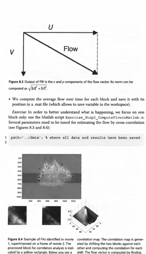
Figure 8.3 Output of PIV is the x and y components of the flow vector. Its norm can be computed as

llull

2 +

llvll

2

•

• We compute the average flow over time for each block and save it with its position in a .mat file (which allows to save variable in the workspace).

Exercise: In order to better understand what is happening, we focus on one

block only: use the Matlab script Exercise_ Step2 _ ComputeFlowinMa tlab. m. Several parameters need to be tuned for estimating the flow by cross-correlation (see Figures 8.3 and 8.4):

1 path=' .. /data'; % where all data and results have been saved

2 700 800 900 1000 100 200 400 600 800 1000 1200

Figure 8.4 Example of FAs identified in movie

1, superimposed on a frame of movie 2. The processed block for correlation analysis is indicated by a yellow rectangle. Below you see a zoomed view of this region for frames 1 and 2 (blocks 1 and 2), and the corresponding

correlation map. The correlation map is generated by shifting the two blocks against each other and computing the correlation for each shift. The flow vector is computed by finding the position of this peak (i.e., the shift where the correlation of blocks 1 and 2 is maximal).

(12)

3 %% Set the parameters for the PIV (normalized correlation based)

4 Correlation_windowsize=16; % block size for normalized correlation

5 Correlation_overlap=B; % the correlation will be computed every Correlation_overlap pixels

6 Correlation_Max_search_area=S; % To add if the expected displacement is bigger than the block size

7 Correlation_threshold=0.3; % only score above this value will

be kept to measure the flow

8 %(max theoretical value =1.0 for two identical images)

9 maxspeed=S; % Maximum velocity allowed {in pixel per frame): this parameter will allow to crop

10 %the correlation map between two blocks to avoid false peaks. code/Step2_ ComputeFlowinMatlab.m

Try different parameters for the window size (8, 16, 32, and 64): comment on both accuracy of results and speed of computation.

8.4.2

Summary of Tools Used in Step 2 and Alternative Tools

qui ver is a native Matlab function to smooth and plot vector data as arrows (see example in Figure 8.5). norxcorr2 is a native Matlab function allowing to compute correlation (similarity) map. The position of its maximum can be found using the max Matlab function returning both the position and the value of the maximum.

•

"

'

•

• I

_•

• _.

_-

• ••

"

✓

• --

,

• _"'

~

_I

J

..

_--

_•

~

'

~

,"'-

~

,.._

Figure 8.S Output of the quiver visualization of flow, with scale parameter at 1 O (norm multi- plied by 10).

(13)

save allows to back up a selection of variables from the workspace (here used to save the position of the flow computed). To read back the data, the corresponding function is load.

Alternative roofs: Several plug ins for optical flow estímatíon are bundled with Fiji.

• Flow/ (Analyze> Optic Flow> FlowJ): It is more complete since different methods are implemented, including the one based on intensity conservation equation. However, it is more demanding to use since you have to know the meaning of the several parameters to tweak (http:/ /webscreen.ophth.uiowa. edu/bij/flowj.htm).

• PIV analysis (accessible from Analyze> Optic Flow> PIV analysis). This command implements the block matching correlation technique that we have done in Matlab in this step. This is one of the simplest existing methods of optical flow estimation. This plug-in has the advantage of a simple user inter- face and convenient output but needs long computation time.

• Mpicbg plug-ins implemented by Stephan Saalfeld: Plugins > Optic Flow.

- PMCC block flow looks for the block that gives the maximum correlation

score, as in PIV analysis, hut with a different implementation.

- MSE block flow looks for the matching most similar pixel in a search radius

based on the minimal sum difference (not anymore correlation) between two blocks.

MSE Gaussian flow looks for the matching most similar pixel in search

radius based on the minimal sum difference between a Gaussian neighborhood: block is not square anymore, it has a Gaussian shape.

8.5

Step 3: Calculation of Focal Adhesion Features

Now we want to calculate the following FA features and associate with each FA: area, growth rate, and actin flow speed. We will compute these features for each FA, and create a Matlab "structure array" to store it, that is, a structure for each FA containing these features, organized as an array of FA features. The solution processing all the movies is provided in Solution_Step3_GetFeaturesbyFo- calAdhesions. m.

8.5.1

Workflow

8.5.1.1 Import of Focal Adhesion Masks to Matlab

First, we build a for-loop to import the mask images slice by slice with the imread function (see Figure 8.6).

We convert the gray value intensities (format: uint8 integer) into Booleans with a logical operation:

(14)

Stack of masks (TIF files) 3D matrix of Booleans Import to Matlab

~

il

_LLHJ_~11

_{t t} l I 1 1 l 000000 o o o o o o o O I l 1 1 l O 01 000 O 001000 O 0001 O O 000010 O 00000

Figure 8.6 Import of mask images to Matlab.

Now, each FA pixel is marked with 1 (TRUE) and each background pixel is marked with O (FALSE).

8.5.1.2 Identify Objects

At the moment, the mask matrix just gives us the information regarding which pixel belongs to foreground (FA region, value 1) and which pixel belongs to background region (value O). In the next step, we assign all foreground pixels to a certain FA object with a simple rule: All foreground pixels touching each other in space (xy-direction) and time (z-dírection) belong to the same FA.

You can use the function bwlabeln as illustrated in Figure 8.7. L

=

bwlabeln (m3b) returns a label matrix, L, containing labels for the connected components in m3b (see Figure 8.7). The input image can have any dimension; Lis the same size as m3b. The elements of L are integer values greater than or equal to O. The pixels labeled O are the background. The pixels labeled 1 make up one object; the pixels labeled 2 make up a second object; and so on.

b=bwlabeln(a)

~;~~g~º

;J""""""ó ,,.,. • o '1' • "

..

.

\) o • .,

: :

~

o o o 4

(15)

Now we have identifi ed in dividual FAs . Ea ch FA object is defin ed by its un ique label num ber. Befo re we contin ue wi th cal cul ating featu res of our objects, we have to defin e our F As of interest: We only want to analyze F As that are present in the last time frame. Why? In our experiment, actin flow was measured after collecting the FA time series. Thus, actin flow information is only available for F As that are present in the last time frame. But why did we segment not only the last FA image, but the whole time series? Because we need information from the other frames of the time series to calculate the growth rate for our F As of interest (this will be done later, see Section 8.5.1.3).

To identify our FAs of interest, you can apply the unique function to the last frame. Study the Matlab help to get more information about unique.

As a result, you should have an array of numbers (named selected) containing the labels of all F As that are present in the last frame.

8.5.1.3 Calculate Object Features

The next step is a bit tricky. We have our 3D label matrix (L), the actin flow velocity image (flow), and the array with our FAs of interest (selected). Based on these data, we want first to calculate the area in the last frame for each FA of interest, and also assign a unique number to each FA as a feature (label).

The area feature calculation ís done with the regionprops function. We feed regionprops with the last frame of the label matrix. The calculation of object area is straightforward (read the Matlab help for further information and have a look on the code snippet below).

If implemented correctly, regionprops should give an array of structs (named here stat) with fields Area.

stat=

43xl struct array with fields: Area

To get rid of all FAs that are not present in the last frame, we use the information from the selected array and delete respective elements in the stat array:

stat=stat(selected)

Finally, we add second and third features, the FA label number and the movie number, to the stat array. Import flow data saved in step 2 with the load function. This process of feature calculation as described above can be implemented in a few lines of Matlab code:

1 for i=l:length(stat)

2 stat(i) .label=selectedFA{i);%add FA label number (tag) as feature

3 stat(i) .datnumber=dat;% image number as feature code/Solution_Step3_ GetFeaturesbyFocalAdhesions.m

Next we want to compute the FA growth rate. Since the growth rate is the change of area over time, we first have to calculate FA areas for a certain time window. In the example below, a vector named listareas will collect the FA

(16)

600 580 560

_*

*

540

*

520

_*

500

_*

480

*

460

*

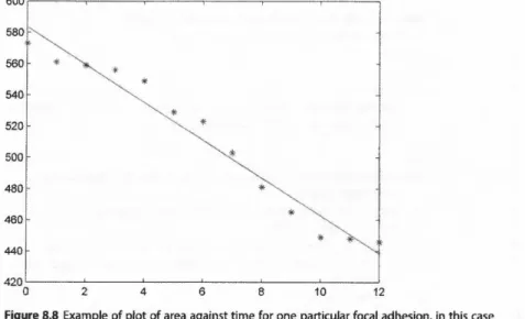
440 420 o 2 4 6 8 10 12

Figure 8.8 Example of plot of area against time for one particular focal adhesion, in this case shrinking.

areas of the last 13 frames (dt). Note that the last value is identical to the feature Area (both are the FA area in the last frame):

>> stat(l) ans=

Area: 282 label: 1 datnumber: 2 >>listareas

listareas =

338 290 280 261 274 269 254 262 271 265 268 282 282

For Matlab experts: Try to calculate the listareas vector on your own. Solu- tion is given in lines 64-68 of the step 3 solution.

Now at each iteration of the loop, we have area profiles over time for each FA. From the area profiles, you can immediately see whether an FA is growing (increase of area over time) or shrinking (decrease of area over time). The area profile of Figure 8.8 shows a shrinking FA.

The growth rate is the change of area over time. This can be calculated, for example, by linear regression of the area profile. Y ou can easily calculate the growth rate(= slope of the area profile) with the following lines:

1 for i=l:length(stat)

2 stat(i) .label=selectedFA(i);%add FA label number (tag) as feature

3 4 5

stat(i) .datnumber=dat;% image number as feature %collect vector of areas for dt time points before

the last frames

(17)

6 7 8 9 10 11 12 13 14

%the growth rate is calculated by linear regression of area values over %time

dt=13; for j=l:dt

isregion=labelsFA(:, :,j+{end-dt}}==stat(i} .label; listareas(j)= sum(isregion(:));

end

listareas(listareas==O)= nan;% FAs may be appearing and then have

%no area {area O) for the first time points. We do not want to fit

%it so we put its values to nan so it will be ignored. x=(O:length(listareas)-1); % create a reference abscissa

for the fit 18 x=[ones(size(x));x}; 15

16 17

19 % to compute the linear regression in this way, we need an additional line at 1

20 p=listareas/x;

21 figure(l) % for visual check

22 plot(x(2, :),listareas,'*'); hold on;

23 plot(x(2, :) ,p{l)+p{2)*x(2, :) , '-r'); hold off; 24 % pis a vector such that p(l)+p(2)*x=listareas 25 stat(i) .growthrate=p(2);

26 end

code/Solution_Step3_GetFeaturesbyFocalAdhesions.m

Finally, we have all our features inside the struct array: stat=

49xl struct array with fields: Area label datnumber growthrate

stat(l) ans=

Area: 503 label: 3 datnumber: 1 growthrate: 14.0659

The last feature we want to add to each FA object is the average flow over time and for the whole FA. In step 2, we have saved in a .mat file per movie the following vector variables: x_pos and y-pos, which are coordinates on one frame, and flow, which is the average flow over time for this position. We start by loading these variables in the workspace:

1 %% Import actin flow data

2 % Calculation of mean actin flow above FA objects to add it as a

3 % feature

(18)

5 % this will load the variables flow, x_pos and y_pos for this dataset

6 % datatoprocess (prefix from 1 to 4) 7 load([path,'/' ,filenameFlowVar));

code/Solution_Step3 _ GetFeaturesbyFocalAdhesions.m

Then for each FA, we add the flow information by computing the average of flow when the pixel in the last frame of the matrix labelsF A at position x_pos and y _pos returns the label number of the current FA processed. Some of the values of flow may have the value nan, because the flow was not computed (too uniform or correlation score of the peak above the correlation threshold allowed in step 2). We use the Matlab function nanmean, which will ignore nan values for computing the mean. (Note: Some nanmean function is provided in the code directory in case you do not have access to the Statistics toolbox.)

1 for Í=l:length(stat) 2 3 4 5 6 7 8 9 10 11 12 13 14 for p=l:length(flow)

% x_pos, y_pos and :fk:M oares fran step2, and are vector with the

% flow magnitude for sparse points on FAs.

% get the list of flow measurement for one particular FA: %collect flow value for this FA:

f=l;

if labelsFA(y_pos(p) ,x_pos(p),end)==stat{i) .label; flowlist{f)=flow{p);

end end

stat(i) .averageflow=nanmean{flowlist); % nanmean STATISTICS TOOLBOX here a version is provided in case Statistics toolbox is not available.

15

16 end

code/Solutíon_Step3_ GetFeaturesbyFocalAdhesions.m We save this array of structure:

1 save([path,'/data_' ,num2str(dat)J ,'stat') code/Solution_Step3_GetFeaturesbyFocalAdhesions.m

8.5.2

Summary of Tools Used in Step 3

Matlab proposes different ways to perform linear regression, or linear fitting. We used the one that was explained in module 2 (c=A/b). Matlab functions in other

(19)

toolboxes (statistics or curve fitting) will also do the job, such as polyfit, regress, or robustfit.

8.6

Step 4: Statistical Analysis

Next, we want to find out whether there are interesting relationships between the features. In particular, the questions we had were the following:

• What is the relationship between growth rate, actin flow, and size?

• Do growing FAs (positive growth rate) exhibit a stronger or weaker actin coupling compared with disassembling FAs (negative growth rate)?

We first collect the data for all movies in one big structure array:

1 path=' .. /data';

2 allstat=[] ;% initialisation in order to append all processed files in one

3 for i=l:4

4 load( [path,' /data_' ,num2str(i)]) 5 length(stat)

6 allstat=[allstat;stat]; 7 end

code/Solution_Step4_Statistica1Analysis.m

We create three vectors (area, flow, and growth rate) that contain in line i the feature for FA i and will be easier to manipulate.

1 for i=l:length(allstat} 2 3 area(i)=allstat(i) .Area; 4 flow(i)=allstat(i) .averageflow; 5 growthrate(i)=allstat(i) .growthrate; 6 end

code/Solution_Step4_Statistica1Analysis.m

We can then plot for each FA its position in area, flow, and growth rate space:

1 plot3(growthrate,area,flow,'o'); hold on;

2

3 xlabel('Area growth (slope)'),

4 ylabel('Area in last time point of movie l'); 5 zlabel('Average flow computed on movie 2');

(20)

Q) -~ 0.5 E § 0.4

"

!? _::,0.3 Cl. E 0.2 o o ~ 0.1

~

Q) o ~100 Cl)

~

o 00 o g o o o o 8 50 9 o o o oº êo o o ~ g, .n.º~~.áß....i o~0_~oo0_o~ o ~ o o o o -50 500 o -100 1000

Area growth (slope) 1500

Area in last time point of movie 1

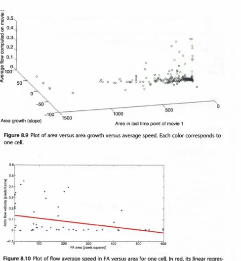
Figure 8.9 Plot of area versus area growth versus average speed. Each color corresponds to

one cell. 0.5

î

¡

0.4 1

i

º-3r

·¡¡ ¡- 1l 02, ; ! ,g ,- _¡; 0.1¡·

i ~

ºl ·

-O.lo'---1,-!-Óo~--~20'--c-o---3-'-oo~---,-'40'--c-o---5,-'-coo~--..,.;600 FA area [pixels squared]

Figure 8.1 O Plot of flow average speed in FA versus area for one cell. ln red, its linear regres-

sion, with a score of 0.12 (not high). More data may be needed to see a relationship.

Figure 8.9 shows the result of a plot of the three main criteria we want to study. From a visual check, it appears that indeed it seems to have an inverse relationship between area and average flow. To check this, we can perform a linear regression on these two measurements (area and flow), as we did previously in step 3 to obtain the growth rate (Figure 8.10). This time, we want to check whether there is a linear relationship between these two features.

1 area=area(~isnan(flow));% we create a subset of area vector which will

2 %contain only area of FAs for which the flow was a number (isnan will return

(21)

3 %1 for each line containing a nan, O otherwise. ~isnan actually do the

4 %contrary ~means NOT in matlab scripting la~guage.

5 %growthrate=growthrate((~isnan(flow))); 6 flow=flow(~isnan(flow)); 7 area=area(flow>0); 8 %growthrate=growthrate(flow>0); 9 flow=fiow(flow>0); 10 11 12 A=fiow; 13 B=[ones(size(area));area]; 14 p=A/B; 15 16 flowfit=p(l)+p(2)*area; 17 figure, 18 19 plot{area,flow,' .')

20 xlabel('FA area [pixels squared]')

21 ylabel('actin flow velocity [pixels/frame]') 22 hold on,

23 plot{area,flowfit,'r-'); 24 flowresid=flow - flowfit; 25 %SSresid is the sum

26 %of the squared residuals from the regression. 27 SSresid=sum{flowresid.A2);

28 %SStotal is

29 %the sum of the squared differences from the mean of the dependent

30 %variable (flow) (total sum of squares). 31 SStotal=sum((flow-mean(flow)) .A2);

32 %This statistic indicates how closely values you obtain 33 %from fitting a model match the dependent variable the model

is intended

34 %to predict. (should be 1 for perfect prediction) 35 rsq=l - SSresid/SStotal;

36 text ( 1000, 3, [' R=' , num2str (rsq) 1 ) ;

code/Solution_Step4_Statistica1Analysis.m

R2 will give the score of the prediction of flow by area using a simple linear regression. The prediction power of flow by area is very low, but would encour- age to get more data since some inverse relationship coherent with the biology behind may be seen.

Exercise:

Now we want to separate assembling and disassembling F As in this analysis. Perform the same fitting by adding two lines before the previous code in order to analyze growing FAs (i.e., growth rate> O). Is the relationship stronger or weaker?

(22)

8.7 Solutions

Full macros and Matlab code are available in the code directory:

• Stepl_FA_segmentation.ijm: Focal adhesion segmentation (ImageJ Macro). • Step2_ComputeFlowinMatlab.ijm: Actin flow computation (Matlab)

• Step3_ GetFeaturesbyFocalAdhesions.m: Calculation of focal adhesion features

(Matlab).

• Step4_StatisticalAnalysis.m: Statistical analysis (Matlab).

References

1 Hu, K., Ji, L., Applegate, KT., Danuser, G., and Waterman-Storer, C.M. (2007) Differential trans mission of actin motion

within focal adhesions. Science, 315 (5808),

111-115.

2 Möhl, C., Kirchgessner, N., Schäfer, C., Hoffmann, B., and Merkel, R (2012) Quantitative mapping of averaged focal adhesion dynami cs in migrating cells by shape normaliza tion. J. Cell Sci; 125 (1), 155-165.

(23)