Calculating the global flux of carbon dioxide into groundwater

Calculating the Global Flux of Carbon Dioxide into Groundwater

Toby Jonathan Kessler B.A., Geology (1998) University of Pennsylvania

Submitted to the Department of Earth, Atmospheric, and Planetary Sciences as Part of the Requirements for the Degree of Master of Science in Geosystems

at the

Massachusetts Institute of Technology May 1999

© 1999 Massachusetts Institute of Technology

All rights reserved

Signature of Author... ... .... ... ....

Dep i t of Earth, Atmospheric, and Planetary Sciences May 10, 1999

Certified by.... ...

Charles F. Harvey Associate Professor of Civil and Environmental Engineering Thesis Supervisor

Accepted by... ...

Ronald G. Prinn, Department Chairman HUSETTS INSTITUTE

Table of Contents

Page

Acknowledgements 3

List of figures and tables 4

Abstract 7

Introduction 8

Background

Global climate change 10

Dissolution of CO2 into water 11

Soils 14

Groundwater recharge 17

Holdridge life-zones 19

Methods

Methods summary 21

Chemistry of carbonate system 23

Data gathering methods

PCO2 28

pH estimation 29

Climate and hydrologic parameters 30

Error in parameters 31 Regressions 32 Depth correction 34 Results 37 Discussion 40 Conclusion 43 Figures 44

Tables (except for table 5: p. 25, and table 9: p. 31) 73

Acknowledgements

Dr. Charles Harvey advised me and provided much of framework for this research and collected most of the papers with PCO2 data. Dr. Michael Follows helped with the

formulation of the chemistry, and with the background about the carbon cycle. The Carbon Dioxide Information and Analysis Center in Oak Ridge, TN, sent several materials related to the carbon cycle, and Rik Leemans sent a database that he created for the Holdridge Life-zone classification system. This thesis was done for the Geosystems master's degree program, and I received numerous pieces of advise from many others

Figures and Tables

Figure 1. Diagram showing the path of CO2 in the ground with the focus of this study at the water table.

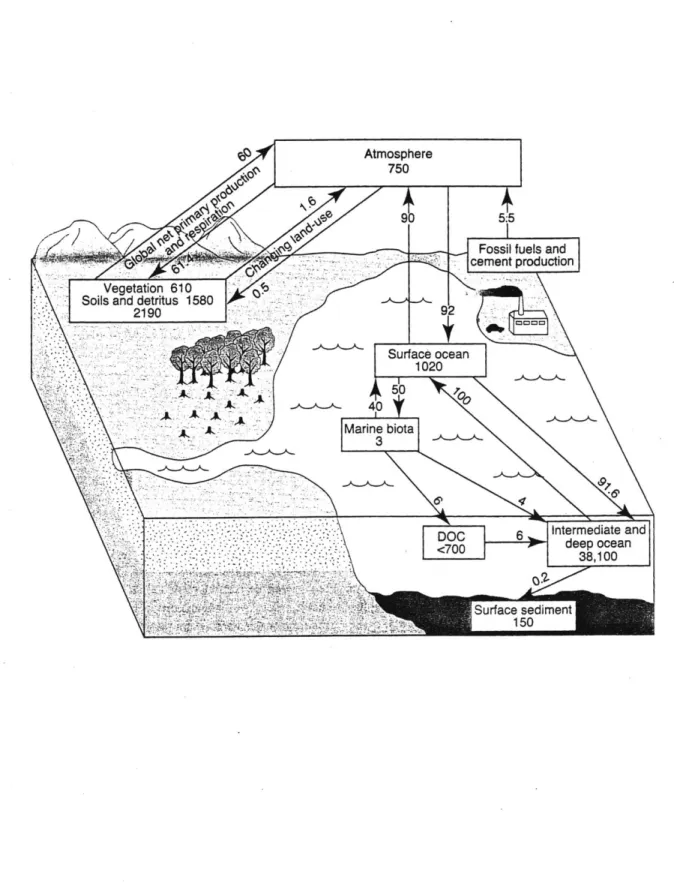
Figure 2. The global carbon cycle, showing the reservoirs in gigatons of carbon (GtC) and fluxes in GtC/y, as annual averages from 1980 to 1989. (Houghton 1995)

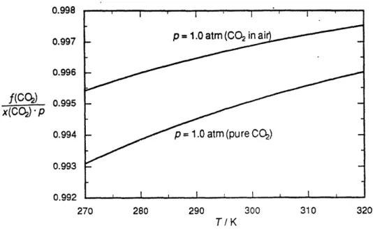
Figure 3. The ratio of fugacity (fCO2) to PCO2 between 270 and 320 Kelvin (DOE 1994)

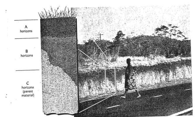
Figure 4. Soil horizons from a road cut in central Africa (Brady 1996)

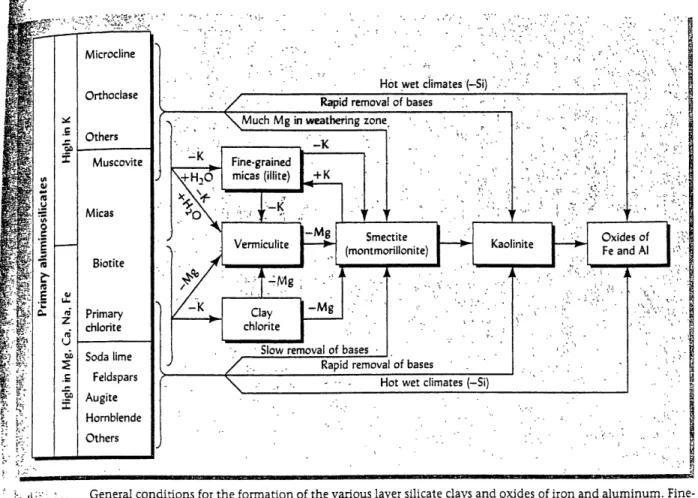
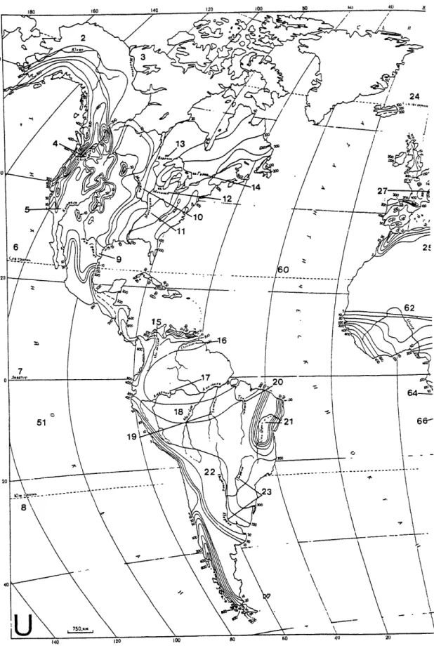
Figure 5. The formation of clays and oxides of iron and aluminum by the weathering of bedrock. Figure 6. Groundwater recharge (R,) for the Western Hemisphere. The larger numbers on the map are

references to particular rivers, and the smaller numbers are R. values in mn/y. The names on the map are in Russian, although the text of the book is translated. (L'vovich 1979)

Figure 7. World map of the Holdridge life-zones (Emanuel 1985)

Figure 8. Classification scheme for the Holdridge life-zones. The vertical axis is temperature and the two diagonal axes are precipitation and potential evapotranspiration ratio. (Holdridge 1972)

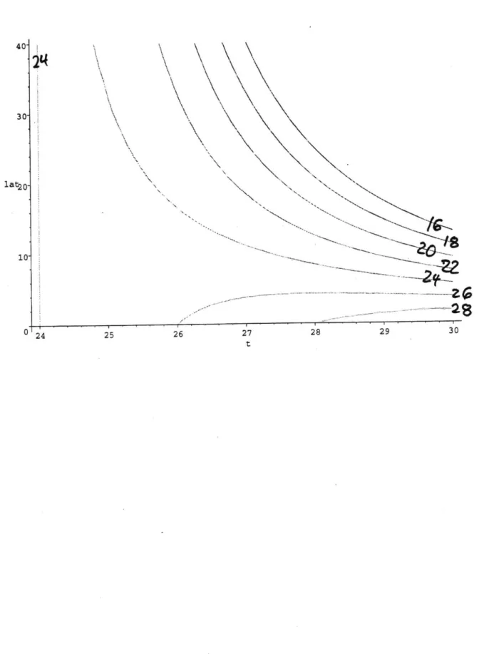
Figure 9. Biotemperature plotted as contours, as a function of temperature and latitude Figure 10. Locations of PCO2 measurements used in this study

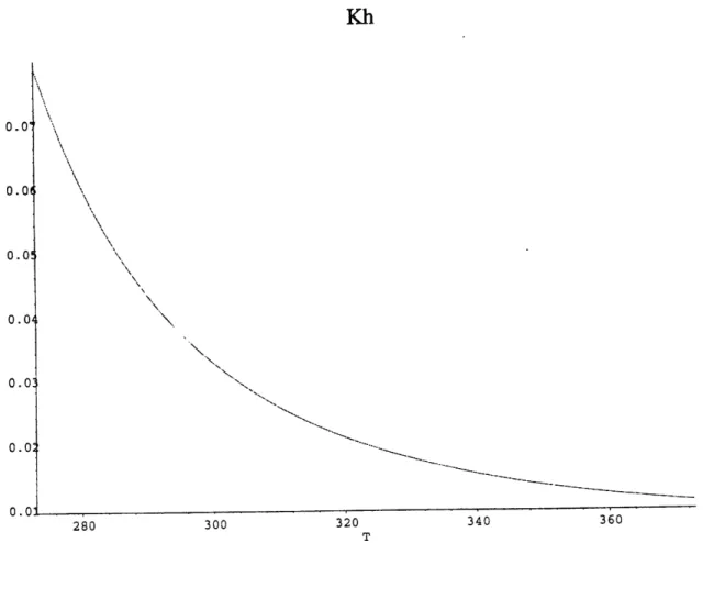
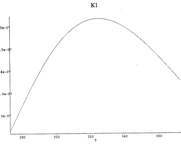
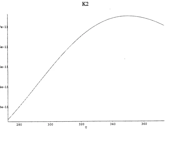
Figure 11. Kh as a function of temperature (Plummer 1982) Figure 12. K, as a function of temperature (Plummer 1982) Figure 13. K2 as a function of temperature (Plummer 1982)

Figure 14. DIC (mol/l) shown in contours, as a function of pH and temperature (K). One can see that for pH below about 5.5, the DIC is not sensitive to changes in pH. For higher pH, DIC is more sensitive to pH changes. Temperature does not have as great an effect.

Figure 15. Geographic distribution of pH in U.S. soils. The bold numbers are means for the selected areas, while the small numbers are county average concentrations. (Holmgren 1993) Figure 16. Land resource areas corresponding to Table 7 (Holmgren 1993)

Figure 17. Generalized soil map of the world from Report No. 66, 1991, FAO, printed in Bridges (Bridges 1997)

Figure 19. Graphs showing PCO2 as a function of depth and time for three different crops grown in Mexico (Buyanovsky 1983)

Figure 20. Contours of PCO2 as a function of depth and time at Brighton, Utah (Solomon 1987) Figure 21. Graph of PCO2 as a function of depth for a soil in Saskatchewan, Canada (Hendry 1993)

Figure 22. Derivation for PCO2 versus depth profile, starting from the assumption of a uniform source of

CO2 throughout the soil profile

Figure 23. PCO2 versus depth, as derived in Figure 22, for a single PCO2 measurement of .01 atm, at a

depth of 2 m, and atmospheric PCO2 = 103-5. The depth of the water table is 30 m.

Figure 24. Composite plot for PCO2 as a function of depth, for data used in this study, with a linear

regression line drawn to fit the data

Figure 25. Carbon Flux per Area, calculated for Holdridge life-zones

Figure 26. Regression for log(PCO2) as a function of precipitation and biotemperature. PCO2 from the

regression is plotted as diagonal contour lines, and the measurements used in this study are plotted as stars

Figure 27. Linear regression between log(PCO2) and precipitation

Figure 28. Linear regression between log(PCO2) and temperature

Figure 29. Carbon flux calculated for the Holdridge temperature-regions (excluding the polar region) Table 1. Geometric means of selected soil elements and associated soil parameters in U.S. surface soils by

taxonomic soil order. (Holmgren 1993)

Table 2. PCO2 measurements and their locations as plotted in Figure 10

Table 3. Complete set of parameters used for the calculations in this study Table 4. Test to show that KIK2/[H*]2

and K,/[H*] are negligible for realistic limits of T, pH, and PCO2 Table 5. (Within text, page 25) Three possible ways of calculating DIC

Table 6. Comparisons between measured and calculated DIC and alkalinity Table 7. PCO2 measurements not used in calculations

V4 -

-Table 9. Properties and nutrients of soils classified in 1974 by FAO[L/NESCO [Sillanpaa, 1982 #18] Table 10. (Within the text, page 31) Error estimation for parameters

Table 11. Total carbon flux in each Holdridge life-zone calculate from PCO2 regression

Table 12. Flux from regressions with PCO2, and from the average DIC for unknown life-zones

Table 13. Global flux and error bounds for different methods Table 14. Total global flux result: summary

Abstract

In this research, the global annual flux of inorganic carbon into groundwater was calculated to be 4.4 GtC/y, with a lower bound of 1.4 GtC/y and an upper bound of 27.5

GtC/y. Starting with 44 soil PCO2 measurements, the dissolved inorganic carbon (DIC)

of the groundwater was determined by equilibrium equations for the carbonate system. The calculated DIC was then multiplied by the groundwater recharge to determine the annual carbon flux per area. These PCO2 estimates were assigned to specific

biotemperatures and precipitations according to the Holdridge life-zone classification system, and regressions between PCO2, biotemperature, and precipitation were used to

provide estimates for regions of the world that lacked PCO2 measurements. The fluxes

were mapped on a generalized Holdridge zone map, and the total flux for each life-zone was found by multiplying the calculated flux by the area in each life-life-zone. While there was a wide range in the error, the calculations in this study strongly suggest that the flux of carbon into groundwater is comparable to many of the major fluxes that have been tabulated for the carbon cycle.

The large flux that was calculated in this study was due to the high PCO2 that is

common in soils. The elevated PCO2 levels are due to the decomposition of organic

matter in soils, and the absorption of oxygen by plant roots. After the groundwater enters into rivers, it is possible that large amounts of CO2 is released from the surface of

-Introduction

CO2 is the most abundant of the "greenhouse gases," and ice core records show

that in the last 100 years, CO2 concentrations in the atmosphere have been 40 percent

higher than they were in the past 18,000 years. In order to understand what the human role has been in changing the atmospheric concentrations of C0 2, it is necessary to

understand the carbon cycle. While many of the human additions to the carbon cycle have been well-documented, researchers have been unable to account for a significant fraction of the anthropogenic carbon. In this research the amount of CO2 that enters into

groundwater has been calculated for the entire Earth's land surface. Since this amount has never been calculated on a global scale, this study gives new results for a piece of the carbon cycle that has been overlooked or considered inconsequential.

There are many intermediate steps involved in transferring carbon from the atmosphere to groundwater (Figure 1), including photosynthesis and decomposition of organic matter. Due to these biological processes in the ground, the partial pressure of CO2 (PCO2) in soils is often 10 times higher than the PCO2 in the atmosphere. The slow

diffusion rate of CO2 out of the ground keeps the PCO2 high in the soil, and this pressure

increases with depth.

In this study, calculations were made for how much CO2 dissolves into the

groundwater for particular areas. For these calculations, the values of CO2 partial

pressures in soils were taken from previous studies, and the amount of CO2dissolved in

the groundwater was found by applying chemical equilibrium equations. The flux of carbon into groundwater for a particular area was then obtained by multiplying the calculated concentration of CO2 by a published rate of groundwater recharge for that area.

The fluxes were then assigned to regions on a worldwide map of Holdridge life-zones, and for life-zones where there was not any PCO2data, regressions with temperature and

precipitation were used to assign PCO. estimates. Fluxes for these unknown life-zones were then computed in the same way as the fluxes for the known PCO2 values.

The results from this study were displayed on a world map that shows the global distribution in the carbon-flux that enters into the groundwater. The global annual sum for this flux was found to be 4.4 gigatons carbon per year (GtC/y), with error estimates giving this value a lower limit of 1.4 GtC/y and an upper bound of 27.5 GtC/y. The magnitude of these results suggests that the flux of carbon into groundwater could have a substantial role in the global carbon cycle.

II. Background

Global Climate Change

In publications since the late 1980's, the Intergovernmental Panel on Climate Change (IPCC) has analyzed a wide array of factors that could lead to global climate change. The greenhouse gases, gases that absorb long-wavelength radiation in the atmosphere, are C02, CO4, CFC's, N20, and No. If we can quantify the increase in concentration of greenhouse gases, we can calculate how much more long-wavelength radiation is being absorbed by the atmosphere. Measurements of greenhouse gases have been made at locations around the world, and these measurements can be compared to the various fluxes in the carbon cycle. By tabulating the human contribution to the greenhouse gases in the atmosphere, IPCC researchers have found numerical values for the degree to which people have contributed to the process of global warming.

The IPCC reports refer to the places that supply carbon to the atmosphere as "sources," and the destinations for carbon leaving the atmosphere as "sinks." "Reservoirs" are places that hold carbon, such as the atmosphere, soil or the ocean, and "fluxes" are the transfer rates between reservoirs. The components of the carbon cycle, including the anthropogenic sources, are shown in Figure 2. The largest global fluxes of carbon is the ocean involve the ocean and the ocean has been found to be a net sink for atmospheric carbon of about 2 GtC/y. Land plants provide the next largest fluxes of carbon since they absorb large quantities of CO2 from the air through the process of

photosynthesis. Land plants are held accountable for a net sink of about 1.4 GtC/y. Human activities that provide sources of atmospheric carbon include the burning of fossil fuel, slash-and-burn agriculture, and other farming practices. The IPCC reports detail the amount that each of these human activities has contributed carbon to the atmosphere, and provide estimates how much of this carbon could leave the atmosphere to various carbon

sinks. Researchers found that their measurements of the concentration of carbon in the atmosphere were different than the predicted values from previously studied carbon sinks. When they made this comparison, they found that there was 1.4 +/- 1.5 GtC less

than they calculated (Houghton 1995). Hence, carbon was leaving the atmosphere to a sink (or many sinks) not considered in the IPCC's calculation.

One should note that Figure 3 leaves out what have been considered to be small parts of the carbon cycle such as groundwater and river water. The inorganic carbon flux from rivers into the ocean, has been published as .3 GtC/y, and the organic carbon flux from rivers into oceans as .4 GtC/y (Suchet 1995). Suchet and Probst calculated that the flux of inorganic carbon from soils into groundwater. Eventually, the carbon from groundwater could make its way into oceans via rivers, be stored below ground in the form of carbonate minerals, or be released from rivers into the atmosphere.

The problem of the "missing sink" remains unsolved. According to the IPCC (Houghton 1995), likely solutions to the missing sink problem include: forest re-growth in the northern hemisphere, increased productivity in plants due to higher concentrations

of CO2in the atmosphere, and higher plant productivity due to the deposition of nitrogen from human pollution. If we do not know where the missing carbon is going, it will be very difficult to make important decisions in a wide array of policy areas such as agriculture and energy usage. We need to understand every aspect of the carbon cycle and how well carbon sinks can absorb the human-derived greenhouse gases.

Dissolution of CO, into water

For carbon dioxide to move from the air to the water, it first dissolves into the aqueous form of CO2. The dissolved CO2then interacts with the other ions in the water.

If there is enough time for these interactions to equilibrate, then the concentrations of the various ions in the water are related by several equilibrium reactions:

CO2 (gas) <--> CO2 (aq) Kh = [C02(aq)] (1)

PCO

C0 2(aq) + H20 (1) <--> H*(aq)+ HC03(aq) K, =

[H+][HCO

i

[CO2(aq)]

HC03(aq) <--> H*(aq)+ C0 32-(aq) K2 = [H.][CO32 (3)

[HCO3.]

The brackets symbolize aqueous concentration, and PCO2 is the partial pressure of CO2 at

the air-water boundary. The PCO2 of a gas in air can be expressed in atmospheres as a

fraction of the total atmospheric pressure, or as a volume-fraction of the air. In the equations above, the K's are the equilibrium coefficients and equation (1) is known as Henry's Law. These K's have a temperature dependence that have been determined through experiments and tabulated by researchers such as Plummer and Busenberg

(1982).

Several details can be noted about these equations: First, the component that is written as, "CO2 (aq)," is actually as combination of CO2 (aq) and H2CO3 (aq), since these

two species are difficult to distinguish. The term, "PCO2," is actually an approximation

for the fugacity, or "fCO2," at the air-water boundary, or the amount of CO2 that interacts

with the water. The fugacity is the partial pressure multiplied by an extra factor, or "fugacity coefficient," that takes into consideration the non-ideal nature of the gases in the air. Since the fugacity coefficients are so close to one (Figure 3), PCO2 was

considered equal to the fugacity for the purposes of this study. Lastly, the "activity," rather than the concentration of each species is what affects the reactions, although for most applications, the activity essentially equals the concentration. Seawater, for instance, has an activity of approximately 0.98, whereas freshwater's activity is nearly one (Drever 1997).

The reactions above describe the open carbonate system, in which water is in contact with air and the various constituents have enough time to equilibrate. The water that was equilibrated with air may migrate below the water table, closing it off from contact with air. Then, the other carbonate species will no longer be affected by Henry's law (equation 1), and new equilibrium concentrations will be reached among the carbonate species in the water. However, the total amount of dissolved, inorganic carbon (DIC) will remain constant, and because of this, it is convenient then to express the amount of CO, in water as the sum of the concentrations of these ions:

[DIC] = [C0 ₂(aq)] + [HCOj(aq)]+ [CO32(aq)] (4)

Provided that the equilibrium coefficients are known, PCO2 is known, and the pH

of the water is known, the DIC can be found from the first three equations above. If the

pH is not known, additional equations are needed to determine the value of [H*]. The

first additional expression is the dissociation of water:

In addition to the total dissolved CO2, another important conservative property in water is alkalinity. Alkalinity is a measure of how sensitive the pH of a solution is to changes in dissolved ion concentration. It can be measured through titration methods, and can also be derived from an expression of charge balance between the positively or negatively charged ions in the soil water:

[Na*] + 2[Mg2 _{] + 2[Ca}2

4] + [H] + [other cations]

= [C-] 2+[SO42] + [HCO3] + 2[CO32_{] + [OH-] + [other anions] (6)}

This equation of charge balance can be rearranged so all of the ions that are strongly affected by pH are on one side of the equation, and this expression is defined as the alkalinity:

Alkalinity = [HCO] + 2[CO32_{] + [OH-] + [other weak anions]}

-[H*] - [other weak cations] (7)

The expression for alkalinity or the expression for charge balance can be combined with the equation (5) to derive the value of [H*], which can then be entered into the equilibrium expression for the reactions involving the carbonate ions. After this algebraic manipulation, the total dissolved CO2 can be found as a function of the known

parameters.

Soils

Soils have many ecological roles, including being a medium for plants to grow in, recycling nutrients and waste, providing a habitat for soil organisms, filtering rain water,

as well as providing the raw material used for farming and construction (Brady 1996). Soils decompose living carbon through microbial decomposition, transforming the carbon from its organic form as solid or dissolved organic matter. The way that soils transfer carbon between organic matter and the atmosphere has been the subject of many carbon-cycle models including the model by van Breeman and others (van Breemen 1990). Soil characteristics that have played a role in these studies include soil texture, temperature, decomposition rates, soil moisture, and time-variations.

What comprises a soil? Soil is defined as the "unconsolidated mineral or organic material at the surface of the earth capable of supporting plant growth," or "the stuff in which plants grow" (Bridges 1997). Liquid and gas components fill the pore space between soil particles, and below a critical depth, the water table, all of the pore space is composed of water. In addition, soils are characterized by soil "horizons," which are layers in the soil that have distinct appearances, textures, and chemical attributes. Figure 4 portrays a picture of a soil profile, with soil horizons labeled as "A," "B," and "C" horizons. These three general horizon types are differentiated as: A) organic rich, B) containing accumulations of minerals, and C) below the root zone, and primarily consisting of weathered bedrock.

Plant and animal materials are decomposed by microorganisms in soils, releasing

C0 2, as well as other gases. In addition, plants absorb oxygen, which increase the fraction

of air which is CO2 (the PCO2). The gases in the soil then slowly mix with the atmosphere through the process of diffusion.

Soil water is sorbed onto clays and other the solid particles, and this water, as well as dissolved ions in the water can be extracted from soil particles by the suction of plant roots. The chemical properties of soils center around the transfer of ions between the soil water (or soil "solution") and to the surfaces of soil solids. Clay minerals, which

comprise a large fraction of the solid particles in a soil, have negatively charged surfaces, and attract the positively charged cations in the soil solution. The quantity of cations that can be bound to the clay minerals, and other soil solids, is called the "cation-exchange capacity," and this quantity depends on the type of clay minerals, and the amount of organic matter in the soil. The particles in soils are weathering products of the soil's "parent material," or bedrock, and have varying cation capacities. Depending on the type of environment, as well as the time that elapses in the weathering process, different clay minerals, and mineral oxides will form in the soil (Figure 5). In addition to clay minerals and mineral oxides, organic colloids that have negatively charged segments can also bind cations in the soil solution.

The pH of a soil solution, or the "soil's pH" is determined by the constituents of the soil solution, as well as by the PCO2 of the soil gas. The cations that lead to an

increase in pH are called "base-cations," and the most predominant of these are Ca2 + and

Mg2_{*, followed by K' and Na*. With the addition of these base cations, the alkalinity of}

the soil solution increases, which buffers the solution from changes in pH. In addition to base cations, "acid-cations" decrease the alkalinity, and tend to lower the pH. The most prominent acid cation is H+, followed by Al3". The ratio of acid to base-cations, rather

than the cation-exchange capacity determines the buffering capacity of the soil solution, and controls the pH in the soil.

Since a soil's pH is determined largely by the type of cations in the soil solution, it is reasonable to expect that different geographic regions would have different chemical constituencies, and thus have different pH measurements in the soil. Indeed, this is the case, and soil surveys both in the United States and around the world have collected large databases for the nutrients in soils as well as the pH for individual soils (Table 1 contains U. S. soil classification orders and the average pH in each soil order). In

addition to geographic differences, there are small pH differences between soil horizons at a particular place, due to varying clay constituents and organic matter of the soil profile. The geographic differences in pH fall under three general descriptions: 1) In warm, humid climates, the pH tends to be very low because all of the base-cations have been weathered out of the soil. As shown on the right side of Figure 5, the highly-weathered parent material leaves only iron and aluminum-oxides, which are composed of predominantly acid-cations. 2) In desert and semi-arid areas, the rapid evaporation of water leaves the soil solution concentrated in base cations such as sodium and calcium, which raises the pH. 3) Finally, in cold, wet places, the decomposition of organic matter occurs at a very slow rate, which leaves the soil solution rich with organic acids, which lowers the pH.

The classification systems used by the Food and Agricultural Organization of the United Nations (FAO) and by the United States Soil Survey share the characteristic that group soils according to diagnostic soil horizons. The soil classifications are structured like biological taxonomic levels, with the highest soil type being the order, followed by suborder, group, and soil series. While there are a few differences, the FAO and the United States soil classifications are very similar, with the FAO having a few more soil orders than the U. S. system, and slightly different names.

Groundwater Recharge

The hydrosphere has many distinct components, the largest of which is the ocean

(96.5%), glaciers (1.74%), and groundwater (1.7%). The remaining water of the hydrosphere is contained in lakes, rivers, and the atmosphere (Shiklomanov 1983). In order to know the rate of water exchange between different components of the

hydrosphere, several equations involving different fluxes need to be solved simultaneously. One representation of these equations is (L'vovich 1979):

P = S + R + E (8)

RIM= S + R (9)

W = P - S = R + E (10)

K = Rg /W (11)

KE = E / W = 1 -KE (12)

E= f(P,E.,) = E. * tanh(P/ E.) (13)

Here, the fluxes of water (in units of volume per area) are: precipitation (P), wetting of the ground (W), evapotranspiration (E, the sum of evaporation and transpiration by plants), total runoff (R,.,), groundwater runoff (Rg), and surface runoff (S). There are two dimensionless parameters in these equations, the groundwater runoff coefficient (Ku) and the evapotranspiration coefficient (KE).

In order to make a map of groundwater recharge worldwide, L'vovich started with measurements of precipitation and total runoff into rivers, and solved for all the other parameters from the above equations. Equation 13) is the most complicated of these equations and is a curve-fit to data. The errors in this interpolation curve range between 2 to 18 percent from measured data taken from different parts of the world. The coefficients Ku and KE derive from other hydrologic computations, and may contain additional errors. After solving these equations for 71 different segments of the Earth's land surface, L'vovich displayed his calculated amounts for groundwater recharge on a

Holdridge Life-zones:

The Holdridge life-zones, shown in Figure 7, correlate environmental parameters with vegetation regions (Holdridge 1972). The two parameters of precipitation and biotemperature determine a location's classification in the Holdridge scheme. The temperature regions are represented as the horizontal rows in the triangular figure, and are named as latitudinal belts ranging from "polar" to "subtropical," an these same regions are classified according to altitudinal descriptions. The third axis of the triangle in Figure 8 is the Potential evapotranspiration ratio (PETR), and is calculated as a function of temperature and precipitation. Life- zones that share the same PETR are labeled as humidity provinces, and range from "semi-parched" to "superhumid." A horizontal dashed line is drawn between the warm-temperate and subtropical temperature regions, separating the life-zones that are prone to frost from the frost-free zones at the bottom of the diagram.

Instead of temperature, or mean annual temperature, the Holdridge life-zone classification uses the quantity, "biotcmperature." Based on the assumption that plants grow most favorably in temperatures ranging from 0 to 300 C, biotemperature is computed by summing the monthly temperatures between 0 and 300 C, then dividing by 12. By defining temperature in this way, places that have high mean annual temperatures actually have slightly lower biotemperatures, and cold places have slightly higher temperatures. In order to bypass the need to collect monthly temperatures, Holdridge published an empirical relation between biotemperature, mean annual temperature and latitude, that applies for mean annual temperatures above 240 C (Holdridge 1972):

Where T is the mean annual temperature in 'C and L is the latitude in degrees. This relationship is shown in Figure 9 as a contour plot, where the x and y axes are Temp and Latitude and contours of biotemperature are shown as curves on this diagram. One can see from Figure 9 that above 240C, biotemperature decreases with increasing temperatures, presumably due to greater seasonal fluctuations of temperature at higher latitudes.

Originally , Holdridge (Holdridge 1947) developed the life-zone system as a way of distinguishing forest types in the tropics, and extended the classification system to the rest of the world. Since the Holdridge life-zones predict vegetation type and climatic conditions, this classification scheme provides an excellent way to relate carbon-cycle data to different terrestrial ecosystems (Kirschenbaum 1996). As an example of a way that the Holdridge classification scheme has been incorporated into carbon-cycle research, Post and others (Post 1982) published their results for the carbon and nitrogen storage held in each life zone, as well as the areas for each of the life-zones.

There are several other classification schemes that predict vegetation types from climatic and hydrologic parameters such as evapotranspiration, temperature, and precipitation. Prentice (Prentice 1992) compared four of these classifications in terms of their ability to predict the vegetation in the land areas for each of these classification schemes, and the classifications differed slightly in terms of the vegetation that they predicted. More recently, Holdridge life-zones have been found to be poor in describing differences in Seasonality (Leeman 1999). Despite its flaws, the Holdridge system was used in this study because of the way in which the Holdridge life-zones are grouped according to temperature and precipitation, and because of the limited accuracy of the calculations.

Methods Summary

The calculations in this study can be summarized by a single equation. The basic equation used in calculating the flux of carbon (per unit area) into groundwater was:

F

=Flux

R-PCO-KK-

1+

+

(15)

Area] 10-pH 10-2pH

In this equation, the parameters on the right include the PCO2, the pH, the groundwater

recharge (Rg), and the equilibrium constants (K,, K2, and Kb). The part of equation (15) to

the right of "Rg" is the equilibrium DIC for a particular location. This part of the equation was determined by the equilibrium chemistry equations, and chosen becau.se the parameters involved could be estimated. The equilibrium DIC was then multiplied by Rg to give the flux per area.

The starting point for this research was PCO, data for soils around the world. Brook and others (Brook 1983) collected PCO2 data from many sources, and published a

world map of soil PCO2 based on regressions with evapotranspiration. This study was

done in the same fashion, and includes much of the PCO2 data published by Brook and

others. Table 2 shows the PCO, measurements with their sources and locations, and these locations are shown on a map in Figure 10. The complete set of parameters used in the study is shown in Table 3. Since the equilibrium constants can be determined from empirical relationships with temperature (Plummer 1982), mean annual temperature data was collected from published sources. After the parameters used in equation (15) were compiled, error estimates were made for each of the parameters involved estimates was used to calculate the error in the results.

While equation (15) gave the carbon flux per unit area for each of the PCO2

carbon flux. Because of the sparseness of PCO2 data around the world (Figure 10),

regressions that involved climatic information was used to correlate regions of the world that shared similar climates but were separated by large distances. The known PCO2

data was regressed against biotemperature and precipitation in order to estimate PCO2 for

regions of the world without PCO2 data. These regressions were used to determine PCO2

values for 23 of the 38 Holdridge life-zones, and with PCO2 values for all of the

Holdridge life-zones, equation (15) gave the total carbon flux for each life-zone. Finally, the total fluxes for each life-zone were summed to give the global flux.

Chemistry of Carbonate System

The goal of using the equilibrium chemistry equations was to determine the amount of dissolved inorganic carbon from the PCO2 data and from other parameters.

The total dissolved inorganic carbon (DIC) in groundwater was found by solving a system of simultaneous equations described above. There are several possible ways to tackle this problem, and the method chosen depends on which of the parameters are known. One of the key assumptions was that the carbonate reactions dominate the equilibrium concentrations of the carbonate species (Butler 1982). Examples of additional reactions that could affect the carbonate system include reactions involving calcium ions (Ca2+), organic compounds, as well as various reactions involving the

dissolution of minerals in the soil or bedrock. These assumptions were tested by comparing empirical measurements to calculations.

If the pH and the PCO2 is known, the DIC can be found by combining the three

equilibrium equations for the carbonate system. It follows from the three carbonate equations (1,2, and 3) that:

[DIC] = Kh(PCO2 {1+ + 2 2 (16)

[Hl

[H*]

In order to use this last expression to find DIC, it is necessary that one knows Kh, PCO2

and [H*]. [H] is found from the pH as 10-pH

Alternatively, one could use an expression for the alkalinity to arrive at a value for DIC, forgoing any measured or assumed value for the pH. To do this, first K, is expressed as:

Kw=

[H([OH-5)

Then, continuing with the assumption that the carbonate reactions dominate the equilibrium conditions (Butler 1982), the alkalinity is then defined as:

Alk = [HCO3-] + 2[CO2(aq)] + [OH - [H*] (17)

Using equation (16), the Alkalinity is then:

Alk = Kh(PCO2 + 1K2 + [ -[H] (18)

Then, this expression can be approximated as:

Alk~ KhKl (P0 2) -[H*| (19)

[H+ ]

This approximation is tested in Table 4, where the terms, (KK 2/[H*]2) and (KJ[H+]), are

shown to be negligible compared to the other terms, for a realistic range of pH and temperatures.

Equations (5) and (19) are then two equations with four variables: Alk, PCO2, [H*], and DIC. [H+] is found by taking the negative log of the pH. The K's are considered constants, and can be found from empirical relations with temperature (Plummer 1982). If any two of these four variables are known, the others can be calculated by solving these two equations simultaneously. There are then three possible

ways to determine DIC from the other variables, and these methods are summarized in Table 5 below. In addition to a combination of the three parameters, PCO2, pH, and

alkalinity, each of these methods also requires an additional parameter, temperature (T) in order to determine the equilibrium constants:

Table 5. Three ways to calculate DIC

Method 1: Start with PCO2, [H+], and T:

[DIC]=

K(PCO

(

+ K + K2K2

(16)

[H+ ] +[H+ ]2)

Method 2: Start with alkalinity (Alk), [H+], and T:

[DIC]

(Alk+ [

H[

1+

KK2

(20)

K I H*

[

Method 3: Start with PCO2, alkalinity (Alk), and T:

+ 2K,

[DIC] =Kh(PCO2). (-Alk + V~(Alk)2 + 4KhKl(PCO2)) (21)

4KIK2

2

(-Alk + j(Alk)2 _{+ 4KhKl(PCO}

2))

In order to choose one of these methods, it was necessary to examine which of the variables were known. It turns out that there is little data about the alkalinity of groundwater or soils. However, the pH of soils has been well documented for a multitude of soil types that have been mapped world-wide. For this reason, method 1 was chosen over methods 2 and 3. If there was a way to estimate a soil's alkalinity based

on its geographic location, method 2 or method 3 could be used to calculate both the

PCO2 in the soil and the dissolved inorganic carbon. If this were the case, method 2

could be used to add information where PCO2 measurements are not available.

An important part of determining which method to use was to estimate the

sensitivity of the calculations to the parameters PCO2,T, and pH. The variation of the

equilibrium constants with temperature was taken from empirical results by Plummer and Busenberg (Plummer 1982): log(K) =108.3865 +.01985076T - 40.45154log(T)+69365 (22) TT2 21834.37 1684915 log(K1)= -356.3094 -. 06091964T + T +126.8339log(T) - (23) 5151.79 5637139 log(K2)= -107.8871-.03252849T + T _TT2+38.92561log(T)- (24)

Figures. 11-13 show how these constants vary between 00 and 300 C. The decrease of Kh

and subsequent increase of DIC at higher temperature is due to the fact that the dissolved

CO2 transforms more readily to a gas at higher temperatures. To see how both pH and temperature affect the DIC values, Figure 14 shows DIC values as contours, for a constant PCO2 of .005 atm. One can see from this figure that for a given temperature,

DIC is not sensitive to changes in pH until the pH increases to about 5 or 5.5. For

example, with T=280 Kelvin (70

C),

In order to test whether it is a valid assumption to ignore any additional reactions besides carbonate reactions (1), (2), and (3), it was necessary to find a published source that included more than two of the relevant parameters: pH, alkalinity, DIC, and PCO2.

Table 6 shows the results of these calculations from two different sources. In each of

these cases, the calculated values were fairly closed to their measured values.

One can see from equation (16) above (method 1), that the dissociation of CO2 in water

increases the amount of CO2 that would dissolve from what one would calculate with

only Henry's Law. If only Henry's law is used,

[DIC] = Kh(PCO2 ). (25)

By using the other two equilibrium reactions (2,3), this amount increases by the factor:

S K1 K2K

+ K + 2 .J ₍₂₆₎

The extra amount of dissolved inorganic carbon is due to the reactions that CO2

undergoes in the aqueous phase. As CO2 reacts with water to form HCO3- and C032, the

aqueous CO2, on right side of the reaction described by Henry's law diminishes, and

more CO₂ dissolves until equilibrium is reached. Regardless of the chemistry in the water, the dissociation if CO2 into other dissolved ions increases the DIC from the value

one would calculate by purely using Henry's law. In order to produce a lower bound for DIC, Henry's Law, which only depends on PCO2 and temperature, was used as a

comparison to the results that were obtained by using PCO2, pH and temperature (method

Data Gathering Methods

PCO2:

The PCO2 data originated from a variety of published sources, and in total, 44

PCO2 values were used in the calculations (Table 2 and Figure 10). Wherever possible, the annual averages of PCO2 were used as data for this study, as well as the PCO2

measurements closest to the water table.

Some of the data was set aside at the beginning of the analysis and these fell into two categories: PCO2 measurements taken in carbonate areas, and a group of

measurements from an area with coal and lignite (Table 7). The reason that PCO2 from

areas with carbonate bedrock were set aside was that calcium (Ca2+) and calcium

carbonate (CaCO3) affect the equilibrium conditions in the carbonate system. Only a

small percentage of the world contains carbonate bedrock, and furthermore, coal and other petroleum deposits comprise only a small fraction of the world's bedrock, and were ignored in these calculations.

Researchers have collected PCO2 data for a variety of purposes, including microbial activity in soils (Hendry 1993); soil formation in carbonate terrain (Reardon

1979); chemical evolution of groundwater in glacial terrain (Wallick 1981); and still

others have measured PCO2 in conjunction with isotopic studies to trace the origin of CO2

in soils (Cerling 1991). In none of the papers used in this study, were PCO2 measurements compiled for the purpose of calculating the flux of carbon into the groundwater.

A large amount of the PCO2 data is from North America, there is some from Europe, Australia, Amazon forests in South America, but very little from Africa and large

parts of Asia (Figure 10). The geographic deficiency of the published PCO2 data is due to

a lack of field studies in many parts of the world.

In many field studies, researchers have demonstrated the seasonality of soil PCO2

-If a given paper included data showing the change of PCO2 over time, an average was

taken of the published data, either by eyeballing the average from a graph of the time-evolution of soil PCO2, or by averaging a set of numbers included in the published paper.

pH estimation:

A pH estimate was made for those locations whose PCO2 sources did not include

the pH of the soil or groundwater Depending on the location in the world for such a PCO2 measurement, this estimate was made in different ways.

For different regions in the U.S., Figure 15 shows the average pH (Holmgren

1993). In the article that this figure is published, Holmgren and others also included a

table for the pH values for 9 soil orders (Table 1) in the U.S. soil classification system, as well as a pH averages for different "land resource regions" in the U.S. (Figure 16 and Table 8).

For locations outside the U. S., the FAO soil maps (FAO/UNESCO 1974) were used to determine soil types. Then, the pH was found from Table 9 (Sillanpaa 1982). In order to convert from pH(CaCl2) to pH(H20), Silanpani provides the empirical formula:

pH(H20)= 0.937 + 0.934 pH(CaCl2) (27)

In the cases where the FAO maps were too detailed for the purpose of this study, a generalized soil map of the world in order to make a rough estimate of the soil type was used (Figure 17). Since many of the FAO soil classification units have changed since

1974, it was necessary to compare the descriptions for each of the soil orders in Bridges (Bridges 1997) and in the World Soil Reference Base (FAO/UNESCO 1974). In addition, a world soil map with U.S. soil orders was used to estimate the pH of Holdridge Life-zones (Figure 18).

Climate and hydrologic parameters

For temperature and precipitation data, there were several sources in addition to the sources for PCO2. These included Korzoun (Korzoun 1977) and L'vovitch (L'vovich

1979). For temperature data, the mean annual temperature was taken from these sources.

The biotemperature, which is used in the Holdridge life-zone calculations, is found using the monthly mean temperatures, as discussed in the Background section above. For locations with biotemperatures above 240 C, equation (4) was used to convert the mean annual temperature to biotemperature. For places with mean annual temperatures less than 10 0C, the biotemperature was computed by averaging the monthly mean

temperatures and using zero for the months with temperatures below 00 C. None of these colder regions, however, had a biotemperature that differed by more than 0.50 C from the mean annual temperature.

Whereas the biotemperatures were used to determine the Holdridge life-zones, the mean annual temperatures were used in the calculations for DIC. Seasonal fluctuations in temperature were ignored because at the water table, the temperature does not fluctuate nearly as much as at the surface.

The recharge of groundwater was found from the map in L'vovitch (L'vovich

1979) (Figure 6). Since many researchers now believe that most of the total runoff is

surface runoff, calculations were made with total runoff (R,), in addition to the groundwater runoff (R).

Error in parameters

In order to compute the error in the calculations, estimates were made for the errors in the data gathering techniques, as summarized in the table below:

The reason that some of these errors are in the form of a percentage is that the method used to obtain these parameters was largely guesswork. For instance, when looking at the groundwater recharge map in Figure 6, it is clear that there is a lot of variation in Rg. However, for places with high and low Rg, one can see a local variation in the contours of about 25%. (The contours on the map were described by L'vovitch as having an error between 2 and 18%). For obtaining PCO2 measurements, graphs showing yearly

fluctuations were eyeballed, and leading to a high margin of error, hence the 50% error estimate shown above.

Regressions

For the life-zones that had PCO2 data, the carbon flux was found using equation

(15). In order to make the calculations for the unknown life-zones, pH and recharge

values were assigned to each life zone by using soil and hydrologic maps. Then, it was possible to estimate the carbon flux into groundwater by extending regression curves from the life-zones with known PCO2 measurements. PCO2 was estimated from the

regression curves according to the temperature and precipitation located at the centers of the Holdridge life-zones (Figure 8).

The independent variables in the regressions were precipitation (Precip) and biotemperature (Biotemp), and for each regression, there was one dependent variable,

log(PCO2). Because PCO2 ranged over several orders of magnitudes, log(PCO2) was

used instead PCO2, making the regressions semi-logarithmic instead of purely linear

regressions. These regressions were then compared to the PCO2 regressions from Brook

and others (Brook 1983).

The regressions were made using the least squares method, in which the coefficients were found for a linear relationship between the dependent and independent variables. For the regressions made with between one dependent and one independent variable, such as between PCO2 and temperature, the regression curve could be plotted as

a straight line. For regressions with two independent variables, such as between

log(PCO2) and both biotemperature and precipitation, the regression produced a plane in

the 3-dimensional space by the three parameters.

Since the uncertainty of the known PCO2 and DIC estimates was small compared

to the variations between neighboring points, this uncertainty of the measurements was not used in calculating the uncertainty of the regression curves. Instead, 95% confidence values for the coefficients of the linear fits were used to make rough estimates for the

upper and lower bounds of the results. For the upper bound estimations, the uppermost value of each of the parameters was used in to determine the carbon-fluxes for the known Holdridge life-zones. One exception was temperature, in which the upper temperature limit was used to calculate the lower limit of the DIC, and the lower limit was used to calculate the upper limit of the DIC. For the unknown life-zones, the uppermost coefficients for the 95% confidence interval were used. One possible statistical method that may be used in further calculations is a Monte Carlo simulation, which would help determine the error more precisely. Matlab numerical software provided the regression functions used in these calculations.

In order to further explore the possible bounds of for the calculations in this study, the PCO2 regressions were repeated with three different approaches to the chemistry and

the hydrologic data. The primary calculation was based on the carbonate chemistry involving all three of the carbonate reactions, equations 1,2, and 3, in the Background section above, and the groundwater recharge. The groundwater recharge, from L'vovitch and others (L'vovich 1979), may significantly underestimate the actual water than infiltrates into the ground, so the calculations with "total recharge" give results that are much larger than those made with groundwater recharge. Finally, the calculations made with groundwater recharge and "K only" were made using the simplest process for the dissolution of CO2into water, Henry's law.

Depth Correction

One additional method that was considered for this study was to estimate the

PCO2 at the water table based on a PCO2 measurement higher in the soil profile.

Although this method was not used in the calculations, it is possible that future calculations could involve the correction for depth which is described below.

Because of the slow diffusion rate of C0 2, the air within the soil tends to have a

much higher PCO2 than the atmosphere. However, as is indicated in Figure 1, the

diffusion of CO2 upward and out of the soil causes the PCO2 to decrease towards the surface. Many of the papers that have PCO2 measurements include graphs of PCO2 as a

function of depth, and some show PCO2 as a function of both depth and time (Figures

19-21). A simple model for diffusion of CO2 through the soil was used to derive an expression for the PCO2 at the water table. In this derivation, only the steady state profile of CO2 was considered, since the parameters used in this study are yearly

averages.

The diffusion equation used in this derivation is known as Fick's law, and can be expressed as:

dC

= dfi,, -C(z) (28)

Here, z is depth, C is PCO2, and dfek is the diffusion coefficient. In addition to diffusion the soil was assumed to have a source of CO2 (microbial decomposition of organic

matter) spread evenly throughout the soil profile. The boundary conditions for soil PCO2 were that the concentration was equal to the atmospheric value (10-" atm) at the soil

surface, and for there to be a no-flow boundary-condition at the water table. The derivation for the PCO2 concentration in the soil profile is given in Figure 22, and Figure

23

For a given PCO2 at a particular depth z, the PCO2 at the water table was found to

be:

D2C - D2_{C - Z12Ca + 2zCatD (29)}

z, (-z1 +2D)

where CD is the PCO2 at the water-table, D is the depth of the water table, Ca, is the PCO2

in the atmosphere, and zi is depth of the measured PCO2 in the soil. This is the equation

that could be used to extrapolate a PCO₂ measurement to give an estimate for the PCO2 at

the water table, and the necessary parameters are given this equation

The results of this simple model is supported by the published PCO2 profiles for

individual locations (Figs. 19-21), as well as by a composite plot of the data used in this model (Figure 24). Further, in Figure 21, one can see that the profiles are roughly parabolic in shape. Aberrations from this profile could be due to transient effects related to the growing season. For example, Figure 19 shows PCO2 decreasing with depth

during the summer months, whereas after August, the PCO2 profile in Figure 19 returned

to the steady-state in which PCO2 increases with depth. In the composite plot, Figure 24,

a linear fit between PCO2 and depth is plotted to illustrate that PCO2 increases with depth

even for a wide range of locations.

The validity of the no-flow boundary condition can be illustrated by using the

PCO2 information from Brazil, shown as number 1 in Table 3. By assuming that the

PCO2 of .07 atm. is at the water table, the ideal gas law, PV=nRT, leads to a

gas-concentration of .13 kg/m3_{. With T=300 K, pH=5.8, the DIC is found from equation (16)}

to be .00294 mol/l. With a groundwater recharge of 200 mm/year, this then leads to a flux

of CO2 of .6 kg/m2/year, which is 1.9*10-' kg/m2/s. In order to compare this flux of CO₂

into the groundwater to the flux of CO2 towards the ground surface, one first needs to

find the gradient of PCO2 in the soil. For a first approximation, one can approximate this

atmosphere (PCO2=10-3 ). With the depth of the water table measured as 45 m, the

gradient would then be:

dC .07 atm -. 003 atm .0067 atm -m' ₍₃₀₎

z 10 m

With a diffusion coefficient of .144 cm2/s (Thorstenson 1983), this leads to an upward diffusive flux of 1.7*10-7 kg/m2/s, which is 100 times faster than the downward flux of CO2 into the groundwater.

Unfortunately, very few of the papers with PCO2 data included the depth of the

water table. Rather than arbitrarily guessing what the depth of the water table for most of the PCO2 measurements, this method was not used in the calculations. Since the PCO2

measurements that were used mostly were taken at shallow depths, a correction for the depth of the water table would increase the PCO2 used in equation (15), and increase the

Results

The results from these calculations show that the flux of carbon into groundwater is on the order of 5 GtC per year. The carbon flux per area are mapped in

Figure 25, and the calculations for each Holdridge life-zone are shown in Table 7. The fluxes that were obtained by extending the PCO2 regressions are labeled with an asterisk,

and if there was more than one PCO2 measurement in a life-zone, the resulting fluxes

were averaged. The results shown in the map were made by using the PCO2 regression

for the unknown Holdridge life-zones. The final result for the total global flux was 4.4 GtC/year, with an upper bound of 27.5 and a lower bound of 1.4 GtC/year.

The regression that was used in making the map in Figure 25 is shown as a contour graph in Figure 26 In this figure, the contour lines represent the regressed values for PCO2 from the two dependent variables, biotemperature and precipitation. The

color-bar on the right provides a scale for the contour lines, as well as for the known PCO2

values, plotted as stars. Since the precipitation and temperature parameters estimates were identical for many of the PCO2 measurements, many of the known PCO2's are at the

same location on this map and on the contour plot. Because of this, Figure 26 contains only 27 stars, whereas there were 44 PCO2 measurements. The equation for the fit

between log(PCO2) and Biotemperature and precipitation was:

Log (PCO2)= -2.62 + 0.0192(Biotemp) + 0.000277(Precip), R

2_{= 0.29 (31)}

where Biotemp is in "C and "Precip" is precipitation in mm/year. The small R2 was due to the large spread in PCO2 data. This low R

2 _{motivated an alternative calculation for the}

global carbon flux, in which the DIC values for the unknown life-zones were taken to be the average DIC that was calculated for the 44 PCO2measurements.

As a comparison to the regressions done by Brook and others (Brook 1983), regressions were made with temperature, instead of biotemperature. The results are shown in Figures 27 and 28, and one can see from these figures that the linear regressions were nearly identical to the regressions published by Brook and others. This is not a surprise, since nearly half of the PCO2 measurements used in this study came

from their 1983 paper. The fact that the R2 _{values were significantly lower in this study}

can be attributed to the small amount of data both in this study and the study by Brook and others. Brook and others made their world soil-PCO2 map based on another

regression, with actual evapotranspiration (AET), which they found had a slightly higher R2 _{when regressed against PCO}

2. As a comparison to their study, further regressions may

be done using the AET data, although it is not likely that the results would be very different.

In Figure 29, one can see the flux calculations for the 6 temperature regions in the

Holdridge life-zone classification. Precipitation increases from left to right on this plot, as in the triangular diagram (Figure 8). One can see that the flux increases rapidly from the left into the middle, and then for the life-zones with the most precipitation on the right, the fluxes decrease slightly. This decrease is due to the lower pH values that exist in extremely wet climates. The soils in these climates contain a high percentage of iron and aluminum oxides, as well as a large amount of organic acids, making the pH comparatively low. In arid life-zones, on the left side of Figure 29, the fluxes are lower, but the error bounds are much larger. This is because of the high pH in arid soils and the greater sensitivity of the calculations at higher pH (Figure 14).

For each of the methods involving the carbonate chemistry and recharge values, two ways used to determine the flux for Holdridge life-zones that did not have any known PCO2 data: PCO2regressions and taking the average DIC from all of the known

life-zones. Tables 12 and 13 show the primary results for the regressions for PCO2 and

for averaged DIC. Whereas the PCO2 regression gave a global flux of 4.4 GtC/y, result

from using the average DIC to determine the DIC for unknown life-zone was 5.3 GtC/y.

These two ways for calculating the flux in the unknown life-zones were repeated for the calculations involving the total recharge, and for simplest CO2 dissolution reaction,

Henry's law. For the pure-Henry's law calculation, the global flux was 3.2 GtC/y for the

PCO2 regression and 3.3 GtC/y for the DIC-averaging calculation. For the method using

the total recharge and the three carbonate chemistry reactions, these values for the global flux were 13.7 GtC/year and 19.1 GtC/year. The results for these different methods, as well as estimates for the upper bounds and lower bounds for each calculation, are summarized below in Tables 14.

Discussion

The carbon flux calculated in this study is quite large, and is comparable to several of the major fluxes that have been established for the carbon cycle. For example, primary production on land is shown in Figure 2 to be responsible for a flux of 61.4 GtC/y, respiration on land produces a flux of 60 GtC/y, and fossil fuel production as 5.5 GtC/y (Houghton 1995). The inorganic carbon flux from rivers into the ocean, has been published as .3 GtC/y, the organic carbon flux from rivers into oceans as .4 GtC/y

(Suchet 1995).

There were several ways that the calculation of 4.4 GtC/year is bounded. Through the use of error estimates for the initial parameters, the lower bound for this primary calculation was 1.4 GtC/y. By using only Henry's law to calculate the DIC at the water table, neglecting any dissociation of CO2 into other carbonate ions, the

calculated carbon flux was 3.2 GtC/y, with a lower bound of 1.4 GtC/y. The lower bound calculations show that the flux of carbon into groundwater is a significant part of the carbon cycle. This conclusion is strengthened by the fact that the errors were calculated

by using the extreme limits of all of the parameters to make the calculations of the upper

and lower bounds. While there were errors in the estimates of pH, recharge and in the

PCO2 data, it is unlikely that the maximum of all of these errors occurred at the same

time.

Where, then could 4.4 gigatons per year fit into the carbon cycle? One explanation for why people have overlooked this flux is that CO2 is released into the air

when the groundwater reaches a river. Any measurements for DIC in a river will be less than the DIC in the river's groundwater sources, due to the difference in soil PCO2 and

the atmospheric PCO2 at the river's surface. Suchet and Probst (Suchet 1995) calculated