HAL Id: inria-00540565
https://hal.inria.fr/inria-00540565
Submitted on 27 Nov 2010
HAL is a multi-disciplinary open access
archive for the deposit and dissemination of
sci-entific research documents, whether they are
pub-lished or not. The documents may come from
teaching and research institutions in France or
abroad, or from public or private research centers.
L’archive ouverte pluridisciplinaire HAL, est
destinée au dépôt et à la diffusion de documents
scientifiques de niveau recherche, publiés ou non,
émanant des établissements d’enseignement et de
recherche français ou étrangers, des laboratoires
publics ou privés.
Large p Small n: Inference for the Mean
Piercesare Secchi, Aymeric Stamm, Simone Vantini
To cite this version:
Piercesare Secchi, Aymeric Stamm, Simone Vantini. Large p Small n: Inference for the Mean. 45th
Scientific Meeting of the Italian Statistical Society (SIS), Jun 2010, Padua, Italy. �inria-00540565�
Piercesare Secchi, Aymeric Stamm, Simone Vantini
Abstract We present a new result that enables inference for the mean vector of a multivariate normal random variable when the number p of its components is far larger than the number n of sample units and the covariance structure is completely unknown. The result turns out to be a useful tool for the inferential analysis (e.i. con-fidence region and hypothesis testing) of data up to now mostly studied only within an explorative perspective, like functional data. To this purpose, an application to the analysis of brain vascular vessel geometry is developed and shown.
Key words: Functional data analysis, Testing statistical hypotheses.
1 Introduction
The advent and development of high precision data acquisition technologies in ac-tive fields of research (e.g., medicine, engineering, climatology, economics), that are able to capture real-time and/or spatially-referenced measures, have provided the scientific community with large amount of data that challenge the classical ap-proach to data analysis.
Modern data sets (large p small n data sets, i.e. data sets characterized by a num-ber of random variables that is much larger than the numnum-ber of sample units) con-trast traditional data sets (small p large n data sets, i.e. data sets characterized by a number of sample units that is much larger than the number of random variables)
Piercesare Secchi and Simone Vantini
MOX - Department of Mathematics “Francesco Brioschi”, Politecnico di Milano, Piazza Leonardo da Vinci, 32, 20133, Milano, Italy,
e-mail: [email protected], [email protected] Aymeric Stamm
University of Rennes I, IRISA, UMR CNRS-6074 Campus de Beaulieu, F-35042 Rennes, France, e-mail: [email protected]
2 Piercesare Secchi, Aymeric Stamm, Simone Vantini
that drove the evolution of statistics and data analysis during the last century. This makes all classical inferential tools nearly useless in many fields at the forefront of scientific research and raises the demand for new modern inferential tools that suit this new kind of data. The aim of this paper is to provide statistical tools for the inferential analysis of large p small n data sets.
An active area of statistical research moving in this direction is functional data analysis (FDA). Indeed, in FDA each sample unit is represented by means of a function (e.g. Ramsay and Silverman, 2005; Ferraty and Vieu, 2006). Nowadays, the typical inferential approach of FDA is the projection of the n functions under investigation - virtually belonging to an ∞-dimensional functional space - onto a finite p-dimensional functional subspace with p smaller than n. Roughly speaking, the original FDA is replaced by a classical multivariate analysis that is expected to well approximate the former one. Technically, performing this replacement means implicitly assuming that the image of the random function under investigation (i.e. the space which the realizations of the random function under analysis belong to) coincides with a specific finite p-dimensional functional subspace. This paper is a first attempt to provide inferential tools for the analysis of large p small n data (e.g. functional data) in a basis-free framework (for functional data this means that there are no assumptions on the spaces which the mean function and the auto-covariance function belong to).
The work of Srivastava (2007) moves in the same direction. In this work, some inferential results non depending on strong assumptions on the covariance structure are presented. Unfortunately, these results are asymptotic in both p and n (i.e. large p large n data). This makes them non suitable to perform inferential statistical analysis of large p small n data.
For clarity of exposition, in Section 2 we recall a few well known results about inference for the mean of a multivariate normal random variable; in Section 3, our new results about inference for the mean when the number p of random variables is far larger than the number n of sample units are presented, while in Section 4 an application of the previous results to the inferential analysis of the local radius of the internal carotid artery is reported.
2 Inference for the Mean: State of the Art
The classical approach to inference for the mean µpof a p-variate normal random variable with unknown covariance matrix Σp relies on a famous corollary of the Hotelling’s Theorem that holds when the number n of sample units is larger than the number p of random variables.
Theorem 1 (Hotelling’s Theorem). Assume that (i) X ∼ Np(µp, Σp), (ii) W ∼ Wishartp(m1Σp, m), (iii) X and W are independent, then for m ≥ p:
m− p + 1
mp (X − µp) 0
Corollary 1 (Hotelling’s Corollary). Assume that (i’) {Xi}i=1,...,n∼ iid Np(µp, Σp), then, for n> p: (n − p)n (n − 1)p(X − µp) 0 S−1(X − µp) ∼ F(p, n − p) ,
whereX and S−1 are the sample mean and the inverse of the sample covariance matrix, respectively.
Corollary 1 makes possible the development of inferential tools for the estimate of the mean value of a p-variate normal random variable (e.g. confidence ellipsoidal regions or hypothesis testing) when the number n of sample units is larger than the number p of random variables; there are no assumptions on the covariance matrix Σpthat is only required to be positively definite. Proofs of the previous results can be found, for instance, in Anderson (2003).
In more and more applications, the number p of random variables is far larger than the number n of sample units and the covariance matrix is unknown. Thus, Corollary 1 cannot be used to make inference for the mean in these cases. In the following section we provide a theorem and a corollary that can be used to make inference for the mean when n is finite, p goes to infinity, and the covariance matrix is unknown.
3 Inference for the Mean of Large p Small n Data
Given a real positively semi-definite p × p matrix A with {λi}i=1,...,pand {ei}i=1,...,p being its eigenvalues and eigenvectors respectively, A+= ∑i:λi6=0
1 λieie
0
iis called the Moore-Penrose inverse of A (e.g Rao and Mitra, 1971). Moreover, we indicate with χ1−α2 (m) the (1 − α)-quantile of a random variable with distribution χ2(m).
Theorem 2 (Generalized Hotelling’s Theorem). Assume that: (i) X ∼ Np(µp, Σp);
(ii) W∼ Wishartp(Σp, m) ; (iii) X and W are independent; then, for m≥ 1: lim p→+∞P " (trΣp)2 trΣ2 p (X − µp)0W+(X − µp) ≤ χ1−α2 (m) # = 1 − α .
4 Piercesare Secchi, Aymeric Stamm, Simone Vantini
Corollary 2 (Generalized Hotelling’s Corollary). Assume that: (i’) {Xi}i=1,...,n∼ iid Np(µp, Σp);
then, for n≥ 2: lim p→+∞P " n(trΣp)2 (n − 1) trΣ2 p (X − µp)0S+(X − µp) ≤ χ1−α2 (n − 1) # = 1 − α ,
whereX and S+are the sample mean and the Moore-Penrose inverse of the sample covariance matrix, respectively.
The proof of Theorem 2 and of Corollary 2 can be found in Secchi et al. (2010). This proof is quite technical and - at the moment - it requires some specific regularity assumptions about the asymptotic behavior of Σp.
Note that Corollary 2 is based on the univariate statistics n(X − µp)0S+(X − µp). We named this statistics Generalized Hotelling’s T2since it can be proven (Secchi et al., 2010) that it generalizes Hotelling’s T2= n(X − µp)0S−1(X − µp) that ap-pears in Corollary 1. Indeed, Hotelling’s T2is defined only for n > p ≥ 1 while the Generalized Hotelling’s T2is defined for any n and p such that n ≥ 2 and p ≥ 1, and it coincides with the former when n > p. Strong connections with the univariate tstatistic are discussed in Secchi et al. (2010).
Corollary 2 turns out to be a useful tool for the construction of confidence regions and hypothesis tests for the mean in all practical situations where the number p of random variables is far larger than the number n of sample units (e.g. genetics) or even virtually infinite (e.g. functional data).
A Confidence Region for the mean µpcan be defined as follows:
CRγ(µp) := ( mp: n(trΣp) 2 (n − 1) trΣ2 p (mp− X)0S+(mp− X) ≤ χγ2(n − 1) ) , (1) with γ being the asymptotic confidence level.
Equivalently, an Hypothesis Test for H0: µp= µ0pversus H1: µp6= µ0p with asymptotic significance level α has the following rejection region:
Reject H0in favor of H1if: n(trΣp)2
(n − 1) trΣ2 p
In practice, the use of Corollary 2, requires the computation of the coefficient (trΣp)2/trΣ2p. Two different scenarios may occur:
• The coefficient (trΣp)2/trΣ2pis known even if Σpis not completely known. This occurs, for instance, in any situation where Σp is known up to a multiplying constant (e.g. if Σp= σ2Ipwith unknown σ2, (trΣp)2/trΣ2pturns out to be equal to p, or if [Σp]i j= σ2min(i, j) with unknown σ2, i.e. a discrete time brownian motion, (trΣp)2/trΣ2pturns out to be equal to 3/2).
• The coefficient (trΣp)2/trΣp2is unknown. In this case we proceed by replacing it with an estimate while the confidence level in (1) and the significance level in (2) become approximate; for instance, in Section 4 the estimator(n−2)(n+1)
(n−1)2
(trS)2
trS2− 1 n−1(trS)2
suggested in Secchi et al. (2010) is used.
The case Σp= σ2Ipwith unknown σ2is widely discussed in Srivastava (2007); in that work the distribution of the statistic (p−n+2)nn−1 (X − µp)0S+(X − µp) is detected for any p > n under the assumption Σp= σ2Ip. The results presented in Srivas-tava (2007) are consistent with Corollary 2. Indeed, when Σp= σ2Ip, for p → +∞, the difference between the statistic (p−n+2)nn−1 (X − µp)0S+(X − µp) and the statistic
n(trΣp)2
(n−1) trΣ2
p(X − µp
)0S+(X − µp) converges a.s. to 0, and the limit distribution of the former statistic is a χ2(n − 1), as expected by Corollary 2.
Before showing an application of our results within the context of functional data analysis (e.g. the analysis of the local radius of 65 Internal Carotid Arteries), we want to point out some peculiar features of confidence region (1) and of test (2). Because S+ is positive semi-definite, the confidence region CRγ(µp) - which for n > p is a p-dimensional ellipsoid in a p-dimensional space - turns out to be a cylinder belonging to a p-dimensional space generated by an n − 1-dimensional ellipsoid. Its graphical visualization is of course non trivial. Nevertheless, knowing if a given vector mpof interest belongs to CRγ(µp) is always trivial. Moreover it can be shown that CRγ(µp) is bounded in all directions belonging to the random space Im(S) and thus all projections onto these directions can be used to partially visualize CRγ(µp). For instance, one may use the n − 1 sample principal components (PCs) as natural directions onto which project and visualize CRγ(µp).
Due to the non-null dimension of the random space ker(S) and to the orthogonal-ity between ker(S) and Im(S), we have that the statistics n(trΣp)2
(n−1) trΣ2
p(X − µ0p)
0S+(X − µ0p) in the hypothesis test (2) does not change if µ0pis replaced by µ0p+ µker(S) with µker(S)being any vector belonging to ker(S). This means that it might happen that H0is not rejected even for values of the sample mean X that are “really very far” from µ0pin some direction within ker(S). This is not surprising, because the use of S+implies an exclusive focus on the space Im(S), neglecting all p − n + 1 directions associated to ker(S).
6 Piercesare Secchi, Aymeric Stamm, Simone Vantini
4 An Application to the Radius of Brain Vascular Vessels
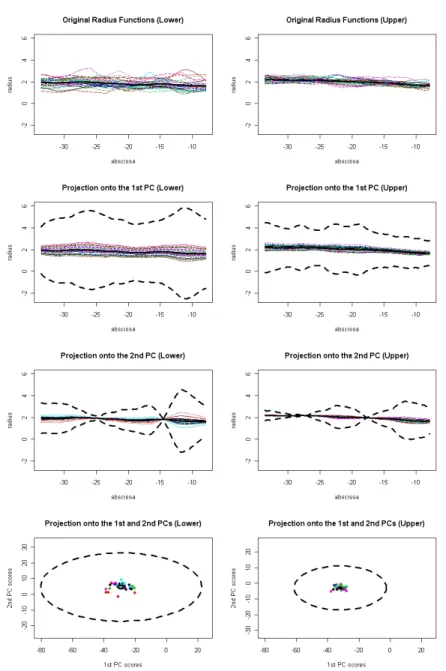
We present here an application of the results introduced in Section 3 to the analysis of a functional data set: the local radius of 65 internal carotid arteries (ICA). Details about the origin and elicitation of these data can be found in Sangalli et al. (2009a) and Sangalli et al. (2009b). The 65 patients are divided into two groups according to the presence and location of a cerebral aneurysm in their brain vascular system: the Lower group (made of 32 patients having an aneurysm along the ICA or healthy) and the Upper group (made of 33 patients having an aneurysm downstream of the ICA). For both groups, a 95% confidence region for the mean radius function and a test for the constancy of the mean radius function are computed.
From a numerical point of view, functional data have been discretized on a suf-ficiently fine grid and the values of the 65 functions in correspondence of the grid points have been used as realizations of the random variables. The grid size (in this case made of 258 points) has been chosen large enough to make the value of the terms on the left of inequalities (1) and (2) stabilize towards their limit values. In practice, we are dealing with two data sets characterized by n = 32 and p = 258, and n = 33 and p = 258, respectively, and the p-asymptotic approximation is going to be used.
In Figure 1, for the two data sets (first row of Figure 1), projections of the radius functions (colored curves) and of the 95% confidence region for the mean function (black dotted curves) along the 1st and 2nd PCs are reported (second and third row of Figure 1, respectively); in the language of multivariate statistics, we would refer to these bounds as the extremities of the T2-simultaneous confidence intervals along the direction indicated by the 1st and 2nd PCs. Similarly to the multivariate case, this representation is not exhaustive, indeed an infinite number of other directions can be explored by means of similar graphics to help the visualization of the confidence region. Note that the fact that a given function lyes within the confidence bounds shown in Figure 1 does not imply that this function belongs to the confidence region (the correct procedure to know if a given function belongs to the confidence region remains using equation (1) directly).
Moreover, note that the bounds in Figure 1 appear to be extremely large com-pared to the variability presented by the data; this is not surprising in a framework where p >> n. To this purpose, in the fourth row of Figure 1, the projection of the 95% confidence region (black dotted ellipse) onto the subspace generated by the 1st and 2nd PCs is compared with the confidence ellipse based on the classical Hotelling’s T2with p = 2 (black full ellipse); this is the confidence region that one would have used if he had projected functional data onto the subspace generated by the 1st and 2nd PCs and had performed - therein - a classical bi-variate statisti-cal analysis neglecting the randomness of the bi-dimensional space onto which the data are projected (i.e. assuming it as deterministically chosen instead of data de-pendent). It is evident that in the framework p >> n, ignoring this randomness can make the actual confidence (or test significance) drift away from its nominal value. Finally, we perform for the two populations a test for checking the constancy of the mean radius, i.e. H0: E[R(s)] = constant versus H1: E[R(s)] 6= constant. This
Fig. 1 First row: radius functions (colored curves). Second and third rows: projections of the radius functions (colored curves) and of the 95% confidence region (black dotted curves) along the 1st and 2nd principal components respectively. Fourth row: projections (by means of PC scores) onto the subspace generated by the 1st and 2nd principal components of the radius functions (colored points) and of the 95% confidence region (black dotted ellipse); for comparison the confidence ellipse based on the classical Hotelling’s T2with p = 2 is reported (black full ellipse). Lower
8 Piercesare Secchi, Aymeric Stamm, Simone Vantini
test is equivalent to the test H0: E[R0(s)] = 0 versus H1: E[R0(s)] 6= 0 that can be performed by applying test (2) to the first derivatives of the radius functions. In par-ticular, the 65 first derivatives have been estimated by means of free-knot regression splines (Sangalli et al., 2009b) and the same grid used to build the confidence regions for the radius functions have been used to perform the test. At the significance level 5%, the null hypothesis of constancy of the mean radius is rejected for the Upper group (p-value < 0.001) and it is not for the Lower group (p-value = 0.076). Thus, a strong statistical evidence for the non-constancy of the mean radius within the last 30 mm of the ICA of patients with an aneurysm downstream of the ICA is found. This conclusion is coherent with the results illustrated in Sangalli et al. (2009a). But - differently from the latter work, where this conclusion is heuristically derived by means of subjective interpretations of functional principal components - in the present work the same conclusion is reached from an inferential perspective where the hypotheses of constancy and non-constancy of radius are formally defined and quantified by means of an hypothesis test procedure.
References
Anderson, T. W. (2003), An introduction to multivariate statistical analysis, Wiley Series in Probability and Statistics, John Wiley and Sons Inc, 3rd ed.
Ferraty, F. and Vieu, P. (2006), Nonparametric functional data analysis, Springer Series in Statistics, Springer, New York.
Ramsay, J. O. and Silverman, B. W. (2005), Functional Data Analysis, Springer New York, 2nd ed.
Rao, C. R. and Mitra, S. K. (1971), Generalized inverse of matrices and its applica-tions, Wiley Series in Probability and Statistics, John Wiley and Sons Inc. Sangalli, L. M., Secchi, P., Vantini, S., and Veneziani, A. (2009a), “A case study in
exploratory functional data analysis: geometrical features of the internal carotid artery,” Journal of the American Statistical Association, 104, 37–48.
— (2009b), “Efficient estimation of three-dimensional curves and their derivatives by free-knot regression splines applied to the analysis of inner carotid artery cen-trelines,” Journal of the Royal Statistical Society, Ser. C, Applied Statistics, 58, 285–306.
Secchi, P., Stamm, A., and Vantini, S. (2010), “Large p Small n: Inference for the Mean,” Tech. rep., MOX, Dip. di Matematica, Politecnico di Milano, work in progress.
Srivastava, M. (2007), “Multivariate theory for analyzing high dimensional data,” Journal of Japan Statistical Society, 37, 53–86.