HAL Id: hal-01457681
https://hal.archives-ouvertes.fr/hal-01457681
Submitted on 3 Aug 2020
HAL is a multi-disciplinary open access
archive for the deposit and dissemination of
sci-entific research documents, whether they are
pub-lished or not. The documents may come from
teaching and research institutions in France or
abroad, or from public or private research centers.
L’archive ouverte pluridisciplinaire HAL, est
destinée au dépôt et à la diffusion de documents
scientifiques de niveau recherche, publiés ou non,
émanant des établissements d’enseignement et de
recherche français ou étrangers, des laboratoires
publics ou privés.
Mediterranean forests under global warming
Cédric Gaucherel, Joel Guiot, L. Misson
To cite this version:
Cédric Gaucherel, Joel Guiot, L. Misson. Changes of the potential distribution area of French
Mediter-ranean forests under global warming. Biogeosciences, European Geosciences Union, 2008, 5 (6),
pp.1493-1504. �10.5194/bg-5-1493-2008�. �hal-01457681�
www.biogeosciences.net/5/1493/2008/
© Author(s) 2008. This work is distributed under the Creative Commons Attribution 3.0 License.
Biogeosciences
Changes of the potential distribution area of French Mediterranean
forests under global warming
C. Gaucherel1, J. Guiot2, and L. Misson3
1INRA, UMR AMAP, TA A.51/PS2, 34398, Montpellier, France
2CEREGE – UMR 6635 CNRS Aix-Marseille Universit´e – BP 80, 13545 Aix-en-Provence Cedex 4, France
3CEFE – UMR 5175 CNRS, 1919 Route de Mende, 34293 Montpellier Cedex 5, France
Received: 14 November 2007 – Published in Biogeosciences Discuss.: 8 February 2008 Revised: 2 July 2008 – Accepted: 21 July 2008 – Published: 4 November 2008
Abstract. This work aims at understanding future spatial and temporal distributions of tree species in the Mediterranean region of France under various climates. We focused on two different species (Pinus Halepensis and Quercus Ilex) and compared their growth under the IPCC-B2 climate scenario in order to quantify significant changes between present and future. The influence of environmental factors such as
atmo-spheric CO2increase and topography on the tree growth has
also been quantified.
We modeled species growth with the help of a process-based model (MAIDEN), previously calibrated over mea-sured ecophysiological and dendrochronological series with a Bayesian scheme. The model was fed with the ARPEGE – MeteoFrance climate model, combined with an explicit
in-crease in CO2atmospheric concentration. The main output
of the model gives the carbon allocation in boles and thus tree production.
Our results show that the MAIDEN model is correctly able to simulate pine and oak production in space and time, after detailed calibration and validation stages. Yet, these simula-tions, mainly based on climate, are indicative and not predic-tive. The comparison of simulated growth at end of 20th and 21st centuries, show a shift of the pine production optimum from about 650 to 950 m due to 2.5 K temperature increase, while no optimum has been found for oak. With the direct
effect of CO2increase taken into account, both species show
a significant increase in productivity (+26 and +43% for pine and oak respectively) at the end of the 21st century.
While both species have different growth mechanisms, they have a good chance to extend their spatial distribution and their elevation in the Alps during the 21st century under
Correspondence to: C. Gaucherel
(gaucherel@cirad.fr)
the IPCC-B2 climate scenario. This extension is mainly due
to the CO2fertilization effect.
1 Introduction
Forest productivity and distribution changes in the coming decades are a major concern of ecological studies. Differ-ential impacts of global climatic changes or increasing
at-mospheric CO2concentration, as well as complex vegetation
feedbacks on climate makes it hard to estimate the vegeta-tion patterns in future (Prentice and Webb, 1998; Sitch et al., 2003). It is particularly true in Mediterranean region which has a limited area but with a high diversity of envi-ronments, vegetation and fauna (Joffre et al., 1999). Forests in this region are crucial for preserving this biodiversity and provide essential ecosystem services, such as soil protec-tion, water conservation and climate regulation (Eamus et al., 2005). Circulation models predict a significant warm-ing and decrease in precipitation in the Mediterranean basin
(Gibelin and Deque, 2003). Giorgi (2006) identified the
Mediterranean basin as the most prominent hot-spot of cli-mate change over the world with more than 20% decline of precipitation over April to September. Precipitation and drought risk changes can trigger a positive feedback on
cli-mate change by decreasing CO2sequestration in ecosystems
(Ciais et al., 2005).
Assessment of climatic change impacts must be supported by accurate and reliable models of climate-vegetation growth relationships (Misson, 2004; Misson et al., 2004; Rathge-ber et al., 2003). These models must be carefully calibrated and validated on data at different time and space scales. At large spatial scales, these data may come from field-based studies on natural gradients (Rathgeber et al., 2005). To
include the time variability at these gradient, dendrochrono-logical series are valuable as an exploratory tool for identify-ing relevant climatic variables and periods when tree growth is responding to climate (Tessier, 1989) or as a support to modelling (Misson, 2004; Rathgeber et al., 2005, 2000). At smaller space and time scale, field data (Rathgeber et al, 2005) and/or coupled micro-meteorological and biogeo-chemical data measured at fine resolution in forest stations (Misson, 2004) are essential to understand eco-physiological processes of the water and carbon cycles in the ecosystem.
Modelling approaches are diverse. Some of them have fo-cused either on ecophysiological processes (Anselmi et al., 2004) or on spatial patterns by the use of statistical rela-tionships (Luoto et al., 2005; Thuiller et al., 2004). We in-tend here to simultaneously investigate both issues. We ex-plore the geographical distribution of two common Mediter-ranean species: Aleppo pine (Pinus halepensis M.) and ever-green Holm oak (Quercus ilex L.) by using an ecophysiolog-ical model (MAIDEN, (Misson et al., 2004) that has been calibrated independently (Gaucherel et al., 2008) for both species using a Bayesian approach. This model is driven here, for the South-East France region, by climate simula-tions for the 21st century, at the daily time step using the Global Climate Model ARPEGE for the IPCC-B2 scenario (Deque et al., 1994). In addition, the fertilization effect of
CO2is assessed by comparing simulations with constant and
with variable CO2concentration.
Our main assumptions for this work are common to other similar works (Yu et al., 2002): forests are mature, they do not genetically adapt to climatic changes, their colonization process is quick enough relatively to climate changes to ne-glect their population dynamics. Moreover, we only focus on potential distribution areas, neglecting human impacts (Debussche et al., 1999). The objectives of this work are threefold: i) to estimate the tendency of both Mediterranean species growth for the 21st century and to compare them to the past (20th century) in order to detect significant changes; ii) to quantify the influence of environmental factors such
as CO2increase on the tree growth according to the
topog-raphy, the other external factors, such as soil composition, being considered as fixed and uniform over the entire region; iii) to quantitatively compare both species behavior
regard-ing to climate/topography/ CO2concentration changes, thus
helping to extrapolate our results.
2 Data and materials
2.1 Dendrochronological and ecophysiological data
We use dendrochronological data from 21 Aleppo pine (P. halepensis) stands (Nicault, 1999) and one typical Holm oak (Q. ilex) stand (unpublished data sampled in the Pu´echabon site (Rambal et al., 2003)). All sites are located
on calcareous soil in PACA region (Long. 0–8◦N×Lat. 41.5–
46.5◦N), southeast France. The pine tree-ring series are
based on the annual earlywood width (Ew), the latewood
width (Lw), the earlywood density (Ed) and the latewood
density (Ld), which are combined into a biomass index,
W (t ) =Ew(t ) .Ed(t ) +Lw(t ) .Ld(t ), taking into account
for both stem radial growth and wood density (Rathgeber et al., 2000). The W (t) curve of oak is calculated on the ring widths only as density measurements are not available. Ring width series are indexed using a digital filter as it is usually done in dendroclimatology (Cook and Kairiukstis, 1990). The oak tree-ring chronology was built by sampling 15 stem disks from 15 trees, among which only seven were kept. Be-cause of the eccentricity of the stem, only the longest radius was measured in each disk. The tree-ring width chronolo-gies on these 15 disks were interdated 2 by 2 in order to give the exact year for each tree ring. Ring with very high and very low width help us interdating the chronologies, as well as rings showing some cell disruption because of very low winter temperature that damaged the cambium (1963, 1985 and 1987). Tree-ring chronologies have been averaged into a 32-year regional chronology (1963–1994) in order to avoid over-parameterization and to perform a rigorous calibration. These 32 years are the common years for all sites. The 38-year oak series (1968–2005) is more local as it is based on a single site. Both mean series will be used to calibrate some parameters of the MAIDEN tree-growth model. Botanical, ecological and topographical factors were also recorded at each stand (Rathgeber et al., 2005) and used to help in cal-ibrating several physiological processes. Two years, 1956 and 1985, are characterized by extremely low winter temper-ature for the region (much below the freezing level), which induced partial damaging of the cambium and had strong im-pacts on the growth during three years. As these processes are not integrated in the model, years 1956–1958 and 1985– 1987 have been removed from the dataset.
In addition, we used the averaged biomass index of each 21 stands over the first 50 years (R50) of each site as an in-dex of the unbiased fertility of the stand. R50 is computed by summing W(t) of each tree over the first 50 years and then av-eraging them over the stand. Although this index could still be influenced by stand density, it offers a synthetic idea of the spatial distribution of pine production (Rathgeber et al., 2005). At two sites, one in P. halepensis and one in Q. ilex,
tree transpirations were measured continuously at1/2h time
step for one year using the heat dissipation method (Granier,
1987). Xylem sap flux density (H2O h−1dm−2 sapwood)
was monitored on 6 trees in the two plots. The sampled trees were representative of the plots’ mean basal area tree circum-ference. The sap flow sensors consist in a pair of probes, 2 cm long and 0.2 cm in diameter each, inserted in a radial orienta-tion separated vertically by 12 cm behind the cambial zone. The temperature difference between the heated and reference probes (1T ) was recorded and sap flux density was calcu-lated according to Granier (1985). Up-scaling from tree to stand was based on the estimation of the stand sapwood area.
2.2 Ecophysiological model
The process-based tree-growth model MAIDEN is exten-sively described in Misson (2004); Misson et al. (2004); Vincke et al. (2005). The model calculates processes such as photosynthesis, stomatal conductance and carbon alloca-tion. The water balance is computed at the ecosystem level, including canopy water interception, transpiration, soil evap-oration, soil water transfer, drainage and runoff. MAIDEN separates daily net primary production (NPP) between car-bon reservoirs (leaf, bole, root and storage) according to phenological phase-dependent rules. These phases are (1) winter: no activity, (2) spring: leaf and root expansion, (3) summer: bolewood production, (4) early falls: carbohydrate-reserve accumulation, (5) late fall: leaf and root senescence. An original modeling procedure of carbon storage and mobi-lization was developed to reproduce the temporal autocorre-lation structure of tree-ring series (Guiot, 1986). The annual increment of bole carbon reservoir at stand level is the mod-eled variable that will be compared with the observed den-drochronological tree-ring series. To be applied to a given species at a given site, the model needs several input vari-ables such as altitude, latitude, maximum absolute Leaf Area Index (LAI), specific leaf area, initial bole biomass, soil thickness and soil textural classes, which can be obtained from site measurements. Moreover, it also needs eleven in-ternal parameters that can be tuned to fit at best available ecophysiological and dendrochronological data, as explained in Gaucherel et al. (2008). Climatic driving variables are daily minimum and maximum temperature and precipita-tions. MAIDEN uses the MT-CLIM algorithm (Running et al., 1987) to estimate daily solar radiation and vapor pressure deficit from daily temperature and precipitations.
2.3 Climatic scenarios
Observed daily temperatures and precipitation series are ob-tained from the METEO-France meteorological station of
Aix-en-Provence. Climatic simulations for the 20th and
21th centuries are obtained from the global climate model ARPEGE-IFS (hereafter APG (Gibelin and Deque, 2003)) driven by the IPCC-B2 scenario radiative forcing (includ-ing greenhouse gases, CO2, CH4, N2O, CFC, water vapor, ozone, and five types of aerosols). Doubling of atmospheric
CO2 concentration occurs towards the end of the 21st
cen-tury with 610 ppm, while the 20th cencen-tury concentrations are the observed values. Description of the model is given in Deque et al. (1994) and Gibelin and Deque (2003). The APG model, for which the time step is 30 min, provides daily max-imum and minmax-imum air temperatures as well as daily precip-itations for the 1960–2099 period. The grid point used has
a 0.5◦×0.5◦cell size that we have interpolated as a function
of latitude and longitude using a two-dimensional (2-D) bi-cubic technique.
We used the Climate Research Unit (CRU) gridded dataset (New et al., 1999) over the 1960–1998 control period to es-timate possible biases of the APG simulation and correct it during the 21st century. This surface climatology has also
a 0.5◦×0.5◦resolution and has been interpolated for
visual-isation comfort in the same way than the APG fields. Al-though having the same resolution, the CRU grid does not perfectly superimpose with the APG grid: to obtain compa-rable data over the whole region, temperature and precipita-tion fields have been systematically corrected by associating the nearest grid points between the two grids (thus without any interpolation). The maximum and minimum tempera-ture and precipitation fields simulated by the APG model are finally compared with the 1960–1998 CRU climatology over South East France (New et al., 1999). In addition, the re-gional topography is available with gridpoints ranging from 0 to 2200 m elevation in Pyrenees and Alps mountains.
3 Methods
3.1 Ecophysiological calibration and simulation
Bayesian techniques such as Monte Carlo Markov Chains (MCMC) offer the opportunity to estimate the (a posteri-ori) distribution of the calibration parameters, starting from their predefined (a priori) statistical distributions (Andrieu et al., 2001; Gelman et al., 1995). We basically proceeded in two main stages (details on the calibration are given in Gaucherel et al., 2008). The a priori distributions are as-sumed to be uniform with a very large range. First, the range of six parameters controlling the ecophysiological processes has been narrowed by using the MCMC algorithm and the transpiration observations available for both species. This method provided us with an a posteriori probability distri-bution and then a 90% confidence interval for each parame-ter. The limits of this interval have been used to define the a priori limits used in the second stage in which the eleven parameters (the six ones calibrated in the first stage, plus the five remaining ones related to carbon allocation processes) have been calibrated on the observed dendrochronological time series. For each calibration, adapted convergence tests proposed by the BUGS project (Spiegelhalter et al., 1993) have been implemented. We performed detailed elasticity tests of the model to estimate possible misspecifications of model’s components, as well as validation on independent meteorological data to detect possible over-parameterization (Gaucherel et al., 2008). Finally, the model fit (determination
coefficient r2)between observations and simulation modes,
after five draws of 5000 steps each, converges and summa-rizes the modeling efficiency.
The eleven parameters are species dependent and valid for the whole region. After the calibration stage, only
cli-matic variables and CO2 atmospheric concentration vary in
r² ~ 0.37 ± 0.04
S tan d ar d iz ed r in g-w id th i n d ic es S tan d ar d iz ed r in g-w id th i n d ic es Time (years)r² ~ 0.50 ± 0.06
(a)
(b)
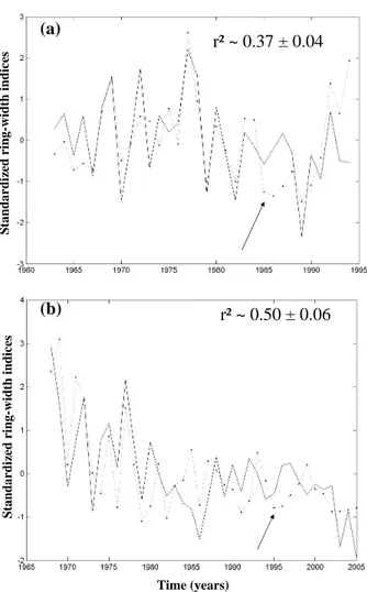
Fig. 1. Indexed tree-ring series (dotted line) and bole carbon
alloca-tion simulated by MAIDEN model after MCMC calibraalloca-tion (plain line) (a) Regional Aleppo pine (Pinus Halepensis) dendrochronol-ogy averaged over 21 series and (b) evergreen oak series at Puech-abon site. Both simulations are based on a calibration stage obtained after the convergence of five draws (5000 steps each). Arrows show excluded years (1985–1986).
topography, elevation and coordinates (for radiative process estimation). We choose averaged regional soil textures for the four soil layers (being 10, 20, 20 and 10 cm deep re-spectively): percentages of clay (25, 30, 35, 35 resp.) and sand (10, 15, 20, 20 resp.) (Misson et al., 2004). Ecophysio-logical simulations are made for mature stands such that the only biomass gain between years is caused by the bole
car-bon allocation. The CO2atmospheric concentration has an
influence on the climate and is taken into account by the cli-mate models, but it has also a direct effect in the tree-growth model, called also fertilization effect because it stimulates the photosynthesis and reduces the water loss through the stomata.
3.2 Regionalization
APG simulations cannot be directly used as inputs in the MAIDEN model because they are affected by some system-atic biases. They have been corrected with the CRU data at every gridpoint and for every month of the studied period, by using the temporal discrepancies between both data sets over the common period (1960–1997). APG temperatures (resp. precipitations) are corrected by adding to daily values the difference (resp. ratio) between APG and CRU means of the corresponding month. No topographical correction has been applied on APG variable values as both data sets present similar topography.
3.3 Simulation validation
R50 index and simulated bole increment for pine species will also be compared in order to assess our model ability to sim-ulate spatial variability of tree-growth, after interpolation us-ing a 2-D bicubic interpolation for southeast France. The assessment of the climate impact on tree-growth is based on the comparison between two periods of 38 years each: 1960– 1997 (hereafter called 20th century period) and 2062–2099
(21st century period). The direct impact of CO2is based on
the comparison on the 21st century with and without
tak-ing into account for the CO2 increase at the input of the
MAIDEN model. Runs without CO2 increase means that
the 1995 CO2concentration (360 ppm) has been used for the
whole 21st century. The vulnerability of both species is as-sessed by comparing the maps of their simulations for both periods and the time series of their averaged bole increments.
4 Results
4.1 Ecophysiological and dendrochronological calibration
The differences (mean absolute values in mm/day) between observed and simulated transpiration over year 2004 is low and reach 4% for pine and 6% for oak (not shown). This discrepancy does not seem to be due to the parameter values as both observation and simulation curves present the same seasonal variations, but rather due to a higher soil depth in-ducing a lower simulation of the soil water stress. The bole
C allocation of the pine is around 650±50 g/mm2and around
250±40 g/mm2for the oak.
The pine MCMC calibration of MAIDEN model with PACA dendrochronological series shows a modal fit at
r2=0.37±0.04 (Fig. 1). This correlation is lower than the
one computed in previous works (Misson, 2004), because model has been improved and because the (Bayesian) cali-bration stage is different and more rigorous (Gaucherel et al., 2008). The oak MCMC calibration of MAIDEN model with the Pu´echabon dendrochronological series shows a modal fit
at r2=0.50±0.06. The agreement between simulated and
Table 1. Monthly values of the three climate parameters used (mean maximum and minimum daily temperatures in◦K and monthly amount of precipitations in mm) for the common period (1960–1997) between CRU (Climatic Research Unit, University of East Anglia) and APG (ARPEGE model M´et´eo-France) data. Corrected APG values using CRU values are noted APG/CRU. Monthly means (for temperatures) and sums (precipitations) are highlighted in bold with their annual means and standard deviations.
Parameters J F M A M J J A S O N D Mean (T◦) or Month
Sum (Pcp) Std T(mean) CRU 2.05 3.09 5.42 8.03 12.01 15.60 18.54 18.18 15.13 10.88 5.74 2.80 9.79 6.09 Tmax APG 4.12 6.10 8.43 11.76 15.70 20.17 23.97 25.37 21.23 14.35 8.56 5.18 13.74 7.54 Tmax APG/CRU 4.75 7.09 10.94 15.80 22.30 28.75 33.87 33.57 25.75 14.72 4.29 −1.40 16.70 12.03 Tmin APG −1.18 −0.52 0.62 2.79 6.09 9.69 12.72 13.43 10.51 5.89 2.52 0.18 5.23 5.28 Tmin APG/CRU −0.55 0.48 3.14 6.83 12.70 18.27 22.62 21.63 15.03 6.26 −1.76 −6.39 8.19 9.71 Pcp CRU 77.85 69.57 69.87 85.48 97.22 85.07 64.30 82.18 91.86 93.84 86.69 80.81 985 10.21 Pcp APG 56.12 47.99 60.40 72.20 95.75 86.70 74.24 58.49 59.85 88.00 82.28 74.73 857 14.91 Pcp APG/CRU 77.83 64.51 86.88 131.32 171.36 129.09 80.43 80.13 87.90 133.44 101.37 77.87 1222 32.10
degraded after, probably under the influence of a biologi-cal factor such as the canopy closure. The model overesti-mated growth in 1996 and 1997, maybe because trees might have shed some leaves during the 1995 extremely dry year. Drought and the reconstruction of the canopy might have ne-cessitated carbohydrates reserves through processes that are not modelled. Conversely, the model seems having overes-timated drought effects in 2003 and 2005. Tree-ring width during the 1999–2005 showed a decreasing trend probably due the accumulation of stress such as increasing drought in the nineties, high temperature in 2003 and insect defoliation in 2004 and 2005. In these circumstances, the model seems to show too much interannual variability and to be unable to solve for low frequency growth cycle.
Nevertheless, differences between calibrated bole incre-ment simulations and observations are quite homogeneous, showing the ability of the model to simulate a large variabil-ity of growth (Fig. 1), while the oak growth is better fitted than the pine growth. It can be due to the negative trend of the oak growth observed since the beginning of the year 70’s. The fact that the model is able to simulate this trend could confirm its climatic origin. As additional and inde-pendent validation, gridded pine R50 values and simulated bole increment are compared and show a correct qualitative agreement (Fig. 2). Maxima are located at the centre of both maps, even if R50 have two maxima and simulation maxi-mum is slightly shifted westward by about 30 km.
4.2 Climate regionalization
Temperature and precipitation data for CRU and APG cli-matology are rather similar over the 38 common years in average (Table 1), but the APG simulations are more
vari-able from month to month. Both temperature data sets
show a lapse rate of about −0.0065 K/m. Spatial tempera-ture and precipitation simulated distribution (not shown) are also more scattered, probably due to the fact that each APG
Longitude (degree) Lat it u d e (d egr ee ) Lat it u d e (d egr ee )
(a)
(b)
S im u lat ed Bol e In cr em en t (g/ m m ²) R 50 P rod u ct ivi ty in d ex (c m )Fig. 2. Map of the simulated bole increments of pine (a) and of the
R50 productivity index (b) in PACA southeast France (inset) for the twentieth century. Coastline is highlighted and the 21 pine stands are superimposed on the R50 productivity index map.
Figure 3
Longitude (degree) Lat it u d e (d egr ee ) Lat it u d e (d egr ee )(a)
(b)
(c)
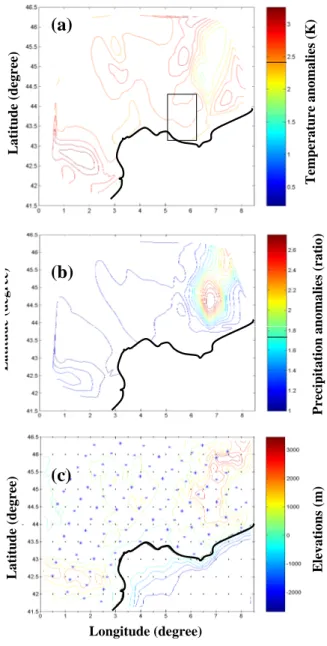
Te m p er at u re a n om al ie s (K ) P re ci p it at ion a n om al ie s (r at io) Lat it u d e (d egr ee ) El evat ion s (m )Fig. 3. (a) Map of the mean temperature anomalies (twenty first
mi-nus twentieth centuries) simulated by ARPEGE and averaged over the 12 months (in K). (b) Map of the precipitation ratios between twenty first and twentieth century simulated by ARPEGE. Daily precipitation ratios have been averaged by month an then over the year. (c) Topography of southeast France, superimposed with the two ARPEGE (dots) and CRU (stars) 0.5◦×0.5◦grids. The 21 pine stand area (Fig. 2) is located on the temperature anomaly map.
gridpoint is a punctual value rather than a cell-grid average. The mean annual deviation (resp. ratio) between APG and CRU datasets over this control period is +3.18±1.68 K for mean temperature (resp. 0.82±0.47 for rainfall) and for the whole studied region. Note that these averaged values are not exactly equal with differences between lines of Table 1, as calculations before averaging stage are made separately for each grid points and each month.
Figure 4
Longitude (degree) Lat it u d e (d egr ee ) Lat it u d e (d egr ee )(a)
(b)
Bol e In cr em en t (g/ m m ²) V ar iat ion s (% )Fig. 4. (a) Map of the mean annual growth of pine in southeast
France at the end of the twentieth century (1960–1997). The mod-ern limit of its potential distribution is indicated in black dashed line. (b) Map of the mean annual growth variation of pine in south-east France (in %), between the twentieth and the twenty first cen-turies without direct effect of CO2(i.e. with atmospheric CO2being fixed to 360 ppm). The 21 pine stand area (Fig. 2) is located on the bole increment map.
APG simulations for the 21st century are corrected using monthly and spatially dependent deviation (or ratio) coef-ficients (Table 2). Temperature (Fig. 3a) and precipitation (Fig. 3b) values of the 2062–2099 period are significantly higher than those of the 1960–1997 period. Mean annual de-viations of daily maximum and minimum temperatures are +2.62±0.66 K and +2.27±0.54 K, respectively, while mean annual precipitation will increase by a factor 1.75±0.98. The temperature diurnal amplitude (max–min) will also decrease with elevation. Precipitation patterns between both periods are very different at high elevations (almost a factor three) and similar at low elevations (Fig. 3b).
Table 2. Correction coefficients (up) of APG parameters for the twenty-first century based on monthly and spatially dependent deviation
(for temperatures) or ratio (for precipitations) coefficients. All coefficients have been computed over the (1960–1997) control period using the whole PACA grid. Mean monthly variations of the corrected climate parameters (down) between the twenty-first and twentieth centuries (noted 21/20) are presented. Annual means and standard deviations of monthly values follow.
Coefficients J F M A M J J A S O N D Mean Std
T(max and min) −0.63 −1.00 −2.52 −4.04 −6.61 −8.58 −9.90 −8.20 −4.52 −0.37 4.27 6.58 −2.96 5.08 Pcp 1.35 1.31 1.45 1.80 1.80 1.51 1.11 1.39 1.46 1.49 1.20 1.04 1.41 0.24
Tmax 21/20 2.54 2.12 2.24 2.49 2.91 2.88 4.16 3.39 2.73 1.94 1.95 2.03 2.62 0.66 Tmin 21/20 2.26 1.89 1.68 1.99 2.16 2.65 3.35 2.95 2.82 1.95 1.68 1.92 2.27 0.54 Pcp 21/20 2.74 4.46 1.83 1.72 1.01 1.14 0.94 1.10 1.67 1.40 1.50 1.53 1.75 0.98
4.3 Pine growth
Pine growth simulated for the 20th century with a CO2
con-centration increasing from 317 ppm (in 1960) to 360 ppm (1995), as expected, shows less productive zones at higher elevations where temperature is less favorable (Fig. 4a). For the 21st century, there will be a negligible mean decrease of about −2.72±4.57% compared to the first period. This hides a large spatial variability with increase up to +8% at high el-evations (Fig. 4b). If we take into account the direct effect
of atmospheric CO2(rising up to 612 ppm at the end of the
21st century), growth pattern will be very different (Fig. 5a): a mean increase of about +22.24±4.14%, with maxima at about +30% at intermediate elevations. Moreover, in rela-tive values, low elevations are the most favored by the direct
fertilizing effect (Fig. 5b). The average gain due to CO2is
about +26.01±3.68% with a significant relative productiv-ity loss of about 0.8% per 100 m elevation (up to the high-est grid-point at elevation 2200 m). This difference between
pine production simulation with and without direct CO2
ef-fect is linear in time and of about 0.34% per year. With CO2
direct effect too, pine production is maximum at intermedi-ate elevation, where the climintermedi-ate is a transition between warm and dry plains and cool and wet mountains (Fig. 5a). Pine growth seems to be optimum nowadays for elevation com-prised below 800 m (Fig. 6a), while this optimum is shifted up to 1100 m for the 21st century (Fig. 6b), whatever is the
CO2factor used. The twenty-year window moving average
curves (Fig. 7a) show that pine growth reaches a maximum
for present if we keep CO2constant during the 21st century,
while it continues to increase if CO2increases according to
the IPCC B2 scenario. The productivity increase seems to be constant, or weakly slowing down, at the end of 21st cen-tury (Fig. 7a). This increase over 100 years reaches 30% in average for the region, with a maximum at intermediate ele-vation. The present distribution of both species only covers a small fraction of these potential areas (approximately 15% for pine and 25% for oak) (Figs. 5a and 8a, dashed lines).
Figure 5
Longitude (degree) Lat it u d e (d egr ee ) Lat it u d e (d egr ee )(a)
(b)
V ar iat ion s (% ) V ar iat ion s (% )Fig. 5. (a) Map of the mean annual growth variation of pine in
southeast France (in %), between the twentieth (1967–1997) and the twenty first (2062–2099) centuries with direct effect of CO2 (increasing from 360 to 612 ppm). (b) Difference of pine growth between simulations with and without increase of CO2 in twenty first century.
Figure 6
Elevation (m) Bol e in cr em en ts ( g/ m m ²)(a)
(b)
(c)
(d)
Fig. 6. Relationships between mean annual growth of pine (resp.
oak) and elevation: (a) pine, twentieth century, (b) pine, twenty first century with CO2direct effect, (c) oak, twentieth century, (d) oak, twenty first century with CO2direct effect. The elevation range where pine and oak are not living at present time is indicated by hashes.
4.4 Oak growth
Simulations of oak growth for 20th century without CO2
di-rect effect show a weak spatial variability and much lower
(two times) productivity than pine (Fig. 8a). Oak mean
growth simulation during the 21st century period decreases by about −13.8±4.8% compared to the control period, but reaches a value of −25% in some low elevation zones (Fig. 8b). The differences between both periods are much more important for oak than for pine. If we include the
di-rect effect of atmospheric CO2(Fig. 9a), mean oak growth
increases by about +24.1±5.6% and reaches a value of about +43% at high elevations. The spatial distribution is quite ho-mogenous regarding to the elevation factor. Oak does not show any optimum with elevation (Fig. 6c, d). The gain due
to CO2direct effect is optimum at low elevations (Fig. 9b).
As highlighted by the twenty-year window moving average
Figure 7 Time (years) Bol e in cr em en t (g/ m m ²) Bol e in cr em en t (g/ m m ²) D rou gh t in d ex (K /d m ) (a) (b) (c)
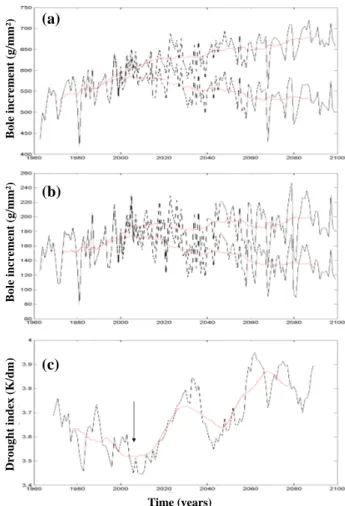
Fig. 7. (a) Evolution of the mean annual production of pine for
southeast France simulated on the basis of the ARPEGE scenario, with (plain line) and without (dotted line) direct effect of CO2. (b) Same for oak. (c) Evolution of a simple drought index (annual
temperature in K divided by annual total of precipitation in mm). The red curves correspond to 20 year window moving averages.
curve, the trend of regional oak growth with and without
CO2 direct effect (Fig. 7b), has the same general behavior
than for pine: a progressive productivity increase
through-out the 21st century with CO2direct effect versus a decrease
with constant CO2. This increase over 100 years reaches
50% in average for the region, and even more at low
ele-vation. Tree growth evolution for constant CO2
concentra-tion reaches a maximum around year 2005 for both species (Fig. 7). The simplified drought index of Fig. 6c (tempera-ture/precipitation ratio) smoothed with a twenty year moving window confirms that the period around 2005 is simulated as the most humid of the analyzed period. Afterwards, drought increases considerably, inducing an important growth deficit
Figure 8
Longitude (degree) Lat it u d e (d egr ee ) Lat it u d e (d egr ee )(a)
(b)
Bol e In cr em en t (g/ m m ²) V ar iat ion s (% )Fig. 8. (a) Map of mean annual growth of oak in southeast France
at the end of the twentieth century (1960–1997); the modern limit of its potential distribution is indicated in black dashed line and the Pu´echabon site is located (red dot). (b) Map of the variation of the mean annual growth of oak in southeast France (in %), between the twentieth and the twenty first centuries without direct effect of CO2 (i.e. with CO2being fixed to 360 ppm).
5 Discussions
5.1 Climate and growth modelling
The distribution of precipitation corrections (computed be-tween CRU and APG data sets for the twentieth reference period) is highly heterogeneous in space (Fig. 3b). This is possibly due to difficulties to precisely simulate frequent and local raining events in Mediterranean climate (West et al., 1986). The precipitation changes are only significantly pos-itive above 500 m, for the benefit to the tree growth. This is obvious for Alps and in a much lower extent for Pyrenees mountains. For temperature, Alps and Pyreneans do not be-have in the same way: temperature anomalies will decrease with elevation in the Alps, and increase in the Pyreneans (not shown), amplifying so the constraints.
Figure 9
Longitude (degree) Lat it u d e (d egr ee ) Lat it u d e (d egr ee )(a)
(b)
V ar iat ion s (% ) V ar iat ion s (% )Fig. 9. (a) Map of the variation of the mean annual growth of
Quer-cus Ilex in Southeast France (in %), between the Twentieth (1967– 1997) and the twenty first centuries with direct effect of CO2 (in-creasing from 360 to 612 ppm). (b) Difference of oak growth be-tween simulations with and without increase of CO2in twenty first century (2062–2099).
The MAIDEN model, after calibration, has shown a cor-rect ability to simulate tree growth of pine and oak species under various environmental conditions (Fig. 1). Some pre-vious works succeeded in such modeling using remote sens-ing (LAI) calibration (Anselmi et al., 2004). Our approach is, in a way, different and original, as we have calibrated a complex ecophysiological model, using dendrochronologi-cal time series (Gaucherel et al., 2008). The simulations are generally realistic from 1960 to 1997. But some short peri-ods (such as 1985–1987) are poorly simulated, mainly due to factors not included in the model, as cold winters that could have damaged the cambium cells of tree bole. The model calibration is based on the mean regional tree-ring chronol-ogy, and an independent validation has been designed on the spatial variability of the tree-growth. The spatial distribution of the pine R50 indices has been successfully compared to the spatial distribution of the simulations.
Tree growth simulations are only regional trends and are still too broad to take into account for detailed abiotic factors such as soil characteristics. Nevertheless, spatial and tempo-ral trends have been clearly identified. If we do not take into
account for CO2fertilization effect, we find that tree growth
has reached a maximum around year 2005 for both species (Fig. 7): this should not be taken as a precise date for the optimum of these species; it rather shows that the climate changes will not beneficiate to these species in the future in terms of ecophysiological processes at large scales in aver-age.
Some assumptions made in this work have to be dis-cussed. Simulated distribution areas are potential distribu-tions, which do not taken into account any history of species colonization nor human influences (Debussche et al., 1999). The present distribution of both species, only covering a small fraction of their potential areas (Figs. 5a and 8a, dashed lines), will likely extend or shift during the coming decades, as it has been simulated for example for broadleaf forests in China by similar approaches (Yu et al., 2002). For clarity too, we have chosen not hiding on maps high elevations at which tree species would not be able to grow due to freeze. Furthermore, another hypothesis behind our results is that there is no population dynamics included in the model, such as metapopulation processes (R´etho et al., 2008), and that species colonization is more rapid than climate dynamics. In case of low colonization rate, the driving factor of the po-tential distribution is no longer the climate, but the disper-sion rate and its modulation by environmental factors (Han-ski and Ovaskainen, 2000). Our simulations, mainly based on climate, are then indicative and not predictive.
5.2 Environmental factors
Topography and climate effects: the pine species produc-tion shows a significant optimum for intermediate elevaproduc-tions (around 650 m, Fig. 6a), indicating that pine does not accom-modate with low temperatures. The oak species production increases with elevation without any optimum, thus directly beneficiating of precipitation increase in mountainous areas (Fig. 6c). Several processes that are not taken into account in our simulations are able to stop the oak progression at higher elevations: competition with other species and embolism of main vessels after winter colds. Our model simulates a shift of the pine production optimum at about 950 m (Fig. 6b), due to 2.5 K temperature increase. This is particularly true if temperature during the warm part of the year is the main control of forest limit in temperate zones (Jobbagy and Jack-son, 2000). Climate is changing, with frost frequencies po-tentially changing too. It is probable that frost will be rarer and will favour colonization at higher elevations too. With this respect, we kept as much information as possible and we did not masked distribution areas computed (Figs. 5 and 9). Finally, both species will be favored during the twenty first century and will likely colonize higher elevations than
occu-pied today, but for different reasons: pine species will climb up because it does not yet reached its productivity optimum, oak species because it probably has no optimum.
CO2concentration: without any direct fertilization effect
of atmospheric CO2, both species show weak changes in
their distribution area: −3 and −14% for pine and oak re-spectively in average for the region (Figs. 4b and 8b). At least is it hard in our simulations to maintain species in plains
(particularly for oak species). With the direct effect of CO2,
both species have a significant increase in productivity: +26 and +43% for pine and oak respectively (Figs. 5b, 9b). This fertilizing effect even, on the basis of our data and model-ing, has a stronger impact than climate change. Higher CO2 concentration allows the tree to close its stomata, leading to a better efficiency in the water use, even if the water budget decreases, such as after year 2030. We are confident about
the simulation of this forcing because CO2fertilizing effect
has been calibrated and validated by using the observed
at-mospheric CO2concentrations for the 20th century. In
addi-tion, the direct effect of CO2tends to reinforce the
produc-tivity/topography relationships and in particular the oak (r2
shifting from 0.38 to 0.54). Finally, the direct effect of CO2
will modify deeply the distribution areas of both species. Both species will certainly maintain in plains at low
eleva-tions, mainly thanks to the CO2fertilization, but this is more
heterogeneous in space for oak species (Figs. 5b, 9b).
5.3 Species comparison (Oak – Pine)
For pine and oak species, productivity increases by about +22 and +26% in the twenty first century under direct effect
of CO2. Both productivities will increase at a rate of about
0.35% per year (Fig. 7). Nevertheless, model simulates a cli-matic optimum elevation at about 1000 m for pine while such optimum is not modeled for oak. This difference is proba-bly due to the way each species beneficiate of temperature and precipitation. These species are representative of two functional types extensively found in the Mediterranean: the oak is an evergreen sclerophyllous often found in secondary successions, and the pine is drought-adapted conifer and a colonizing species. They have a very different physiolog-ical response to drought, which lead to contrasted ecosys-tem functioning: P. halepensis is typically drought-avoiding water-saving, whereas Q. ilex is more tolerant to precipitation variability (Ferrio et al., 2003; Martinez-Ferri et al., 2000; Methy et al., 1997). P. halepensis develops very well in dry environment, but might be less competitive in higher altitude where precipitation is high and temperature is low. Note here that our ecophysiological model does not limit tree growth at high elevations because freeze induced embolism is an effect not taken into account.
Our results also have limitations linked to both data and models. Our measurements still do not cover optimum pe-riods of time. The vegetation models have some lacunae which must be filled up progressively in future. Finally, our
vulnerability studies are based on a single scenario (IPCC-B2) of a single climatic model. They therefore do not have value of prediction but simply of indication. It will be neces-sary, to complete this approach, to use simulation ensembles from several climate models to deal with the climate evolu-tion under probabilistic forms.
6 Conclusion
Finally, considering their present distribution areas being mainly located in the central part of PACA region and at low elevations, pine and oak species have a good chance, according to our data and modeling, to extend their habi-tat. This general trend is mainly (but not only) caused by
the CO2 atmospheric increase. Pine should colonize
east-ward and southeast-ward (along to Alps and Pyrenees slopes), while oak should colonize eastward, in the Alps. While our model does not simulate species competition, nor embolism, the pine productivity optimum with elevation should favor this species in a first stage and then leave the place for oak, in particular at higher (above 1000 m) elevations.
Acknowledgements. We gratefully thank Cyrille Rathgeber and
Yves Gally for comments on earlier drafts or for help in com-puting developments respectively. This research has been funded by the French program GICC2 (Minist`ere de l’Ecologie et du D´eveloppement Durable) (project REFORME, 2005–2007) and by the Agence Nationale de la Recherche (project DROUGHT+, ANR-06-VULN-003-01).
Edited by: J. Leifeld
References
Andrieu, C., Djuric, P. M., and Doucet, A.: Model selection by mcmc computation, Signal Processing, 81, 19–37, 2001. Anselmi, S., Chiesi, M., Giannini, M., Manes, F., and Maselli, F.:
Estimation of mediterranean forest transpiration and photosyn-thesis through the use of an ecosystem simulation model driven by remotely sensed data, Global Ecology and Biogeography, 13, 371–380, 2004.
Ciais, P., Reichstein, M., Viovy, N., Granier, A., Ogee, J., Allard, V., Aubinet, M., Buchmann, N., Bernhofer, C., Carrara, A., Cheval-lier, F., De Noblet, N., Friend, A. D., Friedlingstein, P., Grun-wald, T., Heinesch, B., Keronen, P., Knohl, A., Krinner, G., Loustau, D., Manca, G., Matteucci, G., Miglietta, F., Ourcival, J. M., Papale, D., Pilegaard, K., Rambal, S., Seufert, G., Sous-sana, J. F., Sanz, M. J., Schulze, E. D., Vesala, T., and Valentini, R.: Europe-wide reduction in primary productivity caused by the heat and drought in 2003, Nature, 437, 529–533, 2005.
Cook, E. R. and Kairiukstis, L. A.: Methods of dendrochronol-ogy, applications in the environmetal sciences, Kluwer Academic Press, Dordrecht, 394 pp., 1990.
Debussche, M., Lepart, J., and Dervieux, A.: Mediterranean land-scape changes: Evidence from old postcards, Global Ecology and Biogeography, 8, 3–15, 1999.
Deque, M., Dreveton, C., Braun, A., and Cariolle, D.: The arpege/ifs atmosphere model – a contribution to the french com-munity climate modeling, Clim. Dynam., 10, 249–266, 1994. Eamus, D., Macinnis-Ng, C. M. O., Hose, G. C., Zeppel, M. J.
B., Taylor, D. T., and Murray, B. R.: Ecosystem services: An ecophysiological examination, Australian J. Botany, 53, 1–19, 2005.
Ferrio, J. P., Florit, A., Vega, A., Serrano, L., and Voltas, J.: Delta c-13 and tree-ring width reflect different drought responses in quer-cus ilex and pinus halepensis, Oecologia, 137, 512–518, 2003. Gaucherel, C., Campillo, F., Misson, L., Guiot, J., and Boreux, J. J.:
Parameterization of a process-based tree-growth model: Com-parison of optimization, mcmc and particle filtering algorithms, Environm. Model. Software, 23, 1280–1288, 2008.
Gelman, A., Carlin, J. B., Stern, H. S., and Rubin, D. B.: Bayesian data analysis, Chapman & Hall, London, 526 pp., 1995. Gibelin, A. L. and Deque, M.: Anthropogenic climate change over
the mediterranean region simulated by a global variable resolu-tion model, Clim. Dynam., 20, 327–339, 2003.
Giorgi, F.: Climate change hot-spots, Geophys. Res. Lett., 33, L08707, doi:10.1029/2006GL025734, 2006.
Granier, A.: Une nouvelle m´ethode pour la mesure du flux de s`eve brute dans le tronc des arbres, Ann. For. Sci., 42, 193–200, 1985. Granier, A.: Evaluation of transpiration in a douglas-fir stand by means of sap flow measurements, Tree Physiology, 3, 309–320, 1987.
Guiot, J.: Arma techniques for modelling tree-ring response to cli-mate and for reconstructing variations of palaeoclicli-mates, Eco-logical Modelling, 33, 149–171, 1986.
Hanski, I. and Ovaskainen, O.: The metapopulation capacity of a fragmented landscape, Nature, 404, 755–758, 2000.
Jobbagy, E. G. and Jackson, R. B.: Global controls of forest line ele-vation in the northern and southern hemispheres, Global Ecology and Biogeography, 9, 253–268, 2000.
Joffre, R., Rambal, S., and Damesin, C.: Functional attributes in mediterranean-type ecosystems, in: Handbook of functional plant ecology, Marcel Dekker Inc., New York, 347–380, 1999. Luoto, M., Poyry, J., Heikkinen, R. K., and Saarinen, K.:
Uncer-tainty of bioclimate envelope models based on the geographical distribution of species, Global Ecology and Biogeography, 14, 575–584, 2005.
Martinez-Ferri, E., Balaguer, L., Valladares, F., Chico, J. M., and Manrique, E.: Energy dissipation in drought-avoiding and drought-tolerant tree species at midday during the mediterranean summer, Tree Physiology, 20, 131–138, 2000.
Methy, M., Gillon, D., and Houssard, C.: Temperature-induced changes of photosystem ii activity in quercus ilex and pinus halepensis, Can. J. For. Res.-Revue Canadienne De Recherche Forestiere, 27, 31–38, 1997.
Misson, L.: Maiden: A model for analyzing ecosystem pro-cesses in dendroecology, Can. J. For. Res.-Revue Canadienne De Recherche Forestiere, 34, 874–887, 2004.
Misson, L., Rathgeber, C., and Guiot, J.: Dendroecological analysis of climatic effects on quercus petraea and pinus halepensis radial growth using the process-based maiden model, Can. J. For. Res.-Revue Canadienne De Recherche Forestiere, 34, 888–898, 2004. New, M., Hulme, M., and Jones, P. D.: Representing twentieth century space-time climate variability. Part 1: Development of a 1961–90 mean monthly terrestrial climatology, J. Climate, 12,
829–856, 1999.
Nicault, A.: Analyse de l’influence du climat sur les variations inter-et intra-annuelles de la croissance radiale du pin d’alep (pinus halepensis mill.) en provence calcaire, Aix-Marseille III, Mar-seille, FR, 1999.
Prentice, I. C. and Webb, T.: Biome 6000: Reconstructing global mid-holocene vegetation patterns from palaeoecological records, J. Biogeogr., 25, 997–1005, 1998.
Rambal, S., Ourcival, J. M., Joffre, R., Mouillot, F., Nouvellon, Y., Reichstein, M., and Rocheteau, A.: Drought controls over con-ductance and assimilation of a mediterranean evergreen ecosys-tem: Scaling from leaf to canopy, Global Change Biol., 9, 1813– 1824, 2003.
Rathgeber, C., Nicault, A., Guiot, J., Keller, T., Guibal, F., and Roche, P.: Simulated responses of pinus halepensis forest pro-ductivity to climatic change and co2 increase using a statistical model, Global Planet. Change, 26, 405–421, 2000.
Rathgeber, C., Nicault, A., Kaplan, J. O., and Guiot, J.: Using a bio-geochemistry model in simulating forests productivity responses to climatic change and co2 increase: Example of pinus halepen-sis in provence (south-east france), Ecol. Model., 166, 239–255, 2003.
Rathgeber, C. B. K., Misson, L., Nicault, A., and Guiot, J.: Bio-climatic model of tree radial growth: Application to the french mediterranean aleppo pine forests, Trees-Structure and Function, 19, 162–176, 2005.
R´etho, B., Gaucherel, C., and Inchausti, P.: Spatially explicit pop-ulation dynamics of pterostichus melanarius i11. (coleoptera: Carabidae) in response to changes in the composition and con-figuration of agricultural landscapes, Landscape and Urban Plan-ning, 84, 191–199, 2008.
Running, S. W., Nemani, R. R., and Hungerford, R. D.: Extrap-olation of synoptic meteorological data in mountainous terrain and its use for simulating forest evapotranspiration and photo-synthesis, Can. J. For. Res.-Revue Canadienne De Recherche Forestiere, 17, 472–483, 1987.
Sitch, S., Smith, B., Prentice, I. C., Arneth, A., Bondeau, A., Cramer, W., Kaplan, J. O., Levis, S., Lucht, W., Sykes, M. T., Thonicke, K., and Venevsky, S.: Evaluation of ecosystem dy-namics, plant geography and terrestrial carbon cycling in the lpj dynamic global vegetation model, Global Change Biol., 9, 161– 185, 2003.
Spiegelhalter, D. J., Thomas, A., and Gilks, W. R.: Bugs, bayesian inference using gibbs sampling, MRC Biostatistics Unit, Cam-bridge, UK, 1993.
Tessier, L.: Spatio-temporal analysis of climate tree-ring relation-ships, The New Phytologist, 111, 517–529, 1989.
Thuiller, W., Lavorel, S., Midgley, G. F., Lavergne, S., and Rebelo, A. G.: Relating plant traits and species distributions along biocli-matic gradients for 88 leucadendron species in the cape floristic region, Ecology, 85, 1688–1699 (1683, 1701), 2004.
Vincke, C., Granier, A., Breda, N., and Devillez, F.: Evapotranspi-ration of a declining quercus robur (l.) stand from 1999 to 2001. Ii. Daily evapotranspiration and soil water reserve, Ann. For. Sci., 62, 615–623, 2005.
West, A. W., Ross, D. J., and Cowling, J. C.: Changes in microbial c, n, p and atp contents, numbers and respiration on storage of soil, Soil Biol. Biochem., 18, 141–148, 1986.
Yu, M., Gao, Q., Liu, Y. H., Xu, H. M., and Shi, P. J.: Responses of vegetation structure and primary production of a forest transect in eastern china to global change, Global Ecol. Biogeogr., 11, 223–236, 2002.