OF THE WINTERTHUR INSURANCE CONVERTIBLE BOND: A STUDY OF THE MODEL RISK '
BY
UWE SCHMOCK
Mathematical Finance
Department of Mathematics, ETH Zurich
KEY WORDS AND PHRASES
WINCAT coupon, Winterthur Insurance, catastrophe bond, storm, hail,
model risk, (generalised) Pareto distribution, generalised extreme value distribution, composite Poisson model, generalised linear model, change-point, peaks over threshold.
ABSTRACT
The three annual 2\% interest coupons of the Winterthur Insurance convertible bond (face value CHF 4 700) will only be paid out if during their corresponding observation periods no major storm or hail storm on one single day damages at least 6 000 motor vehicles insured with Winterthur Insurance. Data for events, where storm or hail damaged more than 1 000 insured vehicles, are available for the last ten years. Using a constant-parameter model, the estimated discounted value of the three WINCAT
coupons together is CHF 263.29. A conservative evaluation, which accounts for the standard deviation of the estimate, gives a coupon value of CHF 238.25. However, fitting models which admit a trend or a change-point, leads to substantially higher knock-out probabilities of the coupons. The estimated discounted values of the coupons can drop below the above conservative value; a conservative evaluation as above leads to substantially lower values. Hence, already the model uncertainty is higher than the standard deviations of the used estimators. This shows the dominance of the model risk. Consistency, dispersion, robustness and sensitivity of the models are analysed by a simulation study.
1 1991 Mathematics Subject Classification. 62P05 (primary); 90A09 (secondary).
CONTENTS
1. Introduction 102 2. Presentation and discussion of the data 107 3. A critical review of a binomial model 109 4. Composite Poisson models with constant parameter 111 4.1. Bernoulli distribution for the knock-out events 113 4.2. Pareto distribution for the knock-out events 116 4.3. Generalised Pareto distribution for the knock-out events 121 5. Testing the constant-parameter Poisson model 126 5.1. Testing for over-dispersion 126 5.2. Testing for time-inhomogeneity 128 6. Fitting a generalised extreme value distribution 129 7. Composite Poisson models with a time-dependent parameter 132 7.1. Linear trend of the parameter 134 7.2. Log-linear trend of the parameter 136 7.3. Square-root linear trend of the parameter 138 7.4. Modified-linear trend of the parameter 139 7.5. Smooth transition of the parameter 140 8. Testing for a positive trend in the Poisson parameter 142 9. Composite Poisson model with a change-point 144 10. Peaks-over-threshold method 147 11. Comparison of the estimated values 152 12. Model robustness and sensitivity analysis 154 13. Model consistency and dispersion analysis 156 Acknowledgements 162 References 162
1. INTRODUCTION
The Swiss insurance company Winterthur Insurance has launched a three-year subordinated 2^% convertible bond with so-called WINCAT coupons,
where CAT is an abbreviation for catastrophe. This bond with a face value of CHF 4 700 may be converted into five Winterthur Insurance registered shares ' at maturity (European-style option) between the 18th and 24th of February 2000. The annual interest coupon of 2|% will not be paid out if on any one calendar day during the corresponding observation period for the coupon at least 6 000 motor vehicles insured with Winterthur in Switzerland are damaged by hail or storm (wind speeds of at least 75 km/h). If the number of insured motor vehicles changes by more than 10%, then the knock-out limit of 6 000 claims will be adjusted correspondingly.
Due to the merger of Winterthur Insurance and Credit Suisse Group on December 15th, 1997, the bond may be converted into 36.5 Credit Suisse Group registered shares at maturity. Due to the conversion right and the rising market value of the Winterthur Insurance registered shares (see [20]), the convertible bond offered a good investment opportunity during its first few months.
Had Winterthur launched an identical fixed-rate convertible bond, then, according to Credit Suisse First Boston's brochure [3], the coupon rate would have been around 0.76% lower (approximately 1.49%). In other words, the investor receives an annual yield premium of 0.76% for bearing a portion of Winterthur's damage-to-vehicles risk. This convertible bond is intended as an instrument to diversify portfolios. The WINCAT coupons are
very suitable for this purpose, because storm and hail damages have only a very small correlation with traditional financial market risk. The European-style conversion right, however, strongly ties the bond to the financial market. It is the intention of Winterthur Insurance to test the Swiss capital market for such products, make investors acquainted with them, and obtain a partial reinsurance through the financial market by securitizing a portion of its damage-to-vehicles risk.
Within the range of designs of catastrophe bonds, the Winterthur Insurance convertible bond with WINCAT coupons "Hail" belongs to the more conservative ones, namely the principal-protected catastrophe bonds. Besides the pure catastrophe bonds, where the coupons and the principal are at risk, another more conservative variant are the deferred catastrophe bonds, where no payment as such is at risk, but the payments may be deferred. This gives the issuer of such a bond an interest-free credit in case of a catastrophe.
Two guiding principles for specifying the conditions of the WINCAT
coupons were simplicity and absence of moral hazard. For the purpose of reinsurance, it would have been interesting for Winterthur Insurance to include a knock-out limit connected to the total number of claims during an observation period. To reduce moral hazard, damage arising from a natural cause was chosen as the triggering event, and the knock-out limit is tied to the number of claims and not to the capital necessary to pay full indemnity to the insured. If an event with at least 6000 claims occurs, then Winterthur Insurance saves the corresponding 2|% coupon interest payment on 399.5 million Swiss francs, which makes C H F 8 988 750 at the corresponding coupon date. On the other hand, according to Winterthur Insurance, CHF 3 000 have to be paid out per claim on the average for motor vehicles damaged by storm or hail. Therefore, when an event with at least 6000 claims occurs, Winterthur Insurance can expect to save up to 50% by means of the WINCAT coupons - a profit from a knock-out event seems extremely unlikely. A possible problem with the knock-out limit can be borderline cases of events with about 6 000 claims when a few insured do not know the exact date of the damage (because they have been on holiday, for example). A way to moderate the severity of such a problem would be a linear reduction of the coupon interest rate from 2\% to 0% between 5 000 and 7 000 claims. However, such a specification would make the product more complex and the statistical analysis for the coupon pricing even more involved.
[19] as well as in Credit Suisse First Boston's brochure [3] and thereby to set standards in product transparency, fairness of pricing and investor education. This enables a scientific discussion of such products and their corresponding pricing methodologies, which in turn helps to enhance transparency and acceptance of such products. To satisfy this aim and to build up the confidence of investors, the various sources of risk of such new products should be made explicit to avoid unpleasant surprises. The present paper seeks to make a contribution in this direction with emphasis on education. Since convertible bonds are well-established securities in the market, a lot of information concerning Winterthur Insurance is contained in the legally binding prospectus [18], which helps the investor to judge the default risk and the possible profits from the European-style conversion right. However, no information (other than the exact legal specification) for estimating the knock-out probability of the WINCAT coupons is given in this legally binding prospectus; in particular, there is no historical data on the subject in the prospectus. Apparently, Winterthur Insurance and Credit Suisse First Boston have been aware of this deficiency; hence their decision to publish [3] and to make the historical data available on the web page [19]. This paper will focus on estimating the risk arising from the WINCAT
coupons, with emphasis on the model risk which is not addressed in [3]. For a discussion of the various disguises of model risk, we refer to [4]. Based on the available historical data, we shall present and work out several models and calculate the discounted value of the WINCAT coupons in every case for
an easy comparison of the various results. For the pricing of the European-style option for converting the bond into Winterthur Insurance registered shares, we refer to [3]. We should mention here, that the current value of the call option depends on the knock-out probability of the last coupon, because the exercise price of the call option is either CHF 4 805.75 (face value of the bond plus last coupon), if the last coupon is paid, or simply the face value of CHF 4 700, if the last coupon is knocked out.
To estimate the risk of the WINCAT coupons, a 10-year history of damage
claims is provided in [3] and [19], see Table 1.1. During this period, a total of 17 events with more than 1 000 damaged vehicles were registered. Of these events, 15 happened during the summer and two were winter storms. None of these events occurred between 1987 and 1989. Only two of the events, which happened on the 21st of July 1992 and the 5th of July 1993, caused at least 6000 claims. Without any sophisticated modelling, this suggests a knock-out probability of 20%, i.e., the expectation of the annual coupon payment would be 80% of the 2|% WINCAT coupon, which is an expected annual yield of 1.8%. Of course, as mentioned in [3, p. 11], this estimate has little statistical significance.
In Section 2 of this note, we present and briefly discuss the available historical data. Section 3 contains a critical review of a simple binomial model. In Section 4 we give a review of the constant-intensity model to estimate the discounted value of the WINCAT coupons. We discuss several
an event causing more than 1 000 adjusted claims actually leads to the knock-out of the coupon. These distributions include the Bernoulli distribution, the Pareto distribution (used in [3]) and finally, as suggested by extreme value theory, the generalised Pareto distribution. According to [18] and Winterthur's web page [19], the length of the observation period for the first coupon is not an entire year as assumed in [3]; therefore we recalculate the discounted value of the WINCAT coupons also for the cases already
considered in [3]. In Section 5 we test the constant-parameter model with respect to over-dispersion and time-inhomogeneity. Since the historical data set is small, we can calculate the corresponding probabilities under the null hypothesis exactly and do not need to utilise asymptotic results for these tests.
TABLE 1.1.
CLAIM NUMBERS OF PAST EVENTS CAUSING OVER IOOO ADJUSTED CLAIMS AS PROVIDED IN [3j AND [19]. D U R I N G I W IWJ. SUCH EVENTS DID NOT OCCUR. SINCE THE NUMBER OF MOTOR VEHICLES INSURED WITH W I N I LR niuR i ENDS TO INCREASE, FORMER ACTUAL CLAIM NUMBERS ARE SET INTO RELATION WFTH THE NUMBER
OF INSURED VEHICLES TO OBTAIN THE NUMBER OF ADJUSTED CLAIMS.
Number of Vehicles insured
Year Date Event Adjusted claims claims index 1987 1.248 1988 1.204 1989 1.161 1990 27. Feb. Storm 1646 1.127 1855 1 395 1 572 1991 23. June Hail 1333 1.104 1472 1114 1230 1992 21. July Hail 8 798 1.098 9660 1085 1 191 1 253 1 376 1 733 1 903 27. 30. 23. 6. 21. 31. 20. 21. 5. 2. 24. 18. 6. 10. 26. 2. Feb. June June July July July Aug. Aug. July June June July Aug. Aug. Jan. July Storm Hail Hail Hail Hail Hail Hail Hail Hail Hail Hail Hail Hail Hail Storm Hail 1993 5. July Hail 6589 1.099 7241 1994 2. June Hail 4802 1.086 5 215 940 1021 992 1077 2 460 2 672 2 820 3 063 1995 26. Jan. Storm 1167 1.067 1245 1 290 1 376 1996 20. June Hail 1262 1.000 1262
Only the most severe event within an observation period matters for the possible knock-out of a WINCAT coupon. In Section 6 we therefore fit
a generalised extreme value distribution to the observed yearly maxima. In Section 7 we present and discuss various models with a time-dependent parameter for the number of events with more than 1 000 adjusted claims. We shall give several reasons why there might be a trend in the data. An investor, who wants to take a possible trend into account, might use one of these models to estimate the discounted value of the WINCAT coupons.
Alternatively, an investor, who prefers a constant-parameter model, can use one of the trend models to create a stress scenario for risk management. These trend models will lead to substantially lower estimates for the values of the WINCAT coupons. In the subsequent section we apply a permutation
test to most of the trend models to test the null hypothesis, that there is no trend, and we explain why a permutation test is not adequate for the remaining model with a square-root linear trend.
In contrast to the continuous-trend models, there can also be a sudden change in the expected event frequency. Such a change-point model is presented in Section 9.
The composite Poisson models discussed in Sections 4-9 make use of the assumption that the event frequency is independent from the event severity, namely the adjusted numbers of claims arising from these events. The corresponding trend and change-point models take only a varying event frequency into account. The peaks-over-threshold method from extreme value theory, which we use in Section 10, provides a convenient way to model a possible trend in the event frequency as well as in the event severity. However, when choosing only one additional parameter for the time-inhomogeneous extension of the peaks-over-threshold model, then those two trends are coupled.
A short discussion of the various values of the WINCAT coupons is given
in Section 11; see Table 11.1 for a comparison. The substantially different values indicate that the model uncertainty is the dominating risk for the evaluation of the discounted value of the WINCAT coupons.
In Section 12 we use a scenario technique to investigate the robustness and sensitivity of the various models with respect to new data. This is done by adding fictitious data for the year 1997 to Table 1.1, namely no event for a favourable scenario or a repetition of the four events from 1992 for a stress scenario. The corresponding changes of the estimated coupon values are given in Table 12.1 for the models under consideration. '
In the last section we check the consistency of the models and investigate the dispersion of the estimated discounted coupon values by a simulation study. For every fitted model - under the assumption that it describes reality
Actually, one hail storm in the area Entlebuch/Sarnen with 1 825 claims was recorded on the 11th of June 1997. Another hail storm hit the town of Lucerne on the 21st of July 1998 and caused 3 085 claims. There were no other events with more than 1 000 claims during the years 1997 and 1998. In this paper, however, we only use the information available at the time the bond was issued.
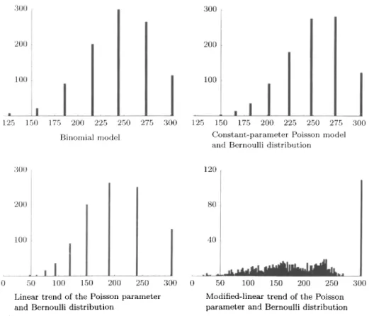
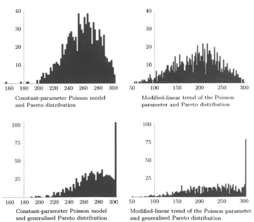
correctly - we generate 1000 new random data sets according to the distribution specified by the fitted model. These data sets replace the actual observations recorded in Table 1.1, and we use the model to estimate the discounted coupon values based on the random data set. In this way we can check whether the model can recover its own features from the simulated data - in particular the mean and the median - and we can see how far the simulated coupon values deviate from the mean. This can help to determine conservative estimates of the coupon values for the models. The mean, the median, the standard deviation and the 15.9%-quantil for the various models are listed in Table 12.1. Instructive are also the histograms in Figures
13.1 and 13.2, showing the distributions of the estimated coupon values for some selected models.
If the knock-out probability PCAT, for the WINCAT coupons were
known exactly, then a very small risk premium for the investor would suffice, because the investor has the freedom to invest only a small fraction of the capital in the Winterthur Insurance convertible bond thereby diversifying the risk. This small risk premium is the motivation for insurance companies to securitize their catastrophe risk. However, the true knock-out probability PCAT is not known. Therefore, at various places in
this paper, we follow the procedure used in [3] and add an estimated standard deviation &(PCAJ) to the estimated knock-out probability PQAT
to obtain a conservative upper estimate, thereby adding a risk premium for the investor to account for the uncertainty of PCAJ- We could elaborate
on this point by using the entire estimated distribution of PCAT and tilt it towards higher values (the paper [17] by G.G. Venter is interesting in this context). Taking investor-dependent utility functions and the current market price of risk into account, a more profound analysis might be possible than the one sketched above. However, since the estimated knock-out probabilities and the corresponding standard deviations will vary substantially with the models used, the model risk should also be taken into account, because is seems to be the dominating one in the present problem. There should be a coherent way to calculate an adequate risk premium which accounts for the variation of the estimated knock-out probability and the corresponding model risk. We leave it to future research to develop a rigorous mathematical basis for this purpose and to apply it to the present problem.
2. PRESENTATION AND DISCUSSION OF THE DATA
Whether a WINCAT coupon is paid on February 28th depends on the events
happening during the corresponding observation period. These observation periods are specified on Winterthur's web page [19], see Table 2.1. The first observation period is shorter than a year so that there are always four months left between the end of the observation period and the coupon
TABLE 2.1.
OBSERVATION PERIODS FOR THE W I N C A T COUPONS ACCORDING TO |i«] AND THE WEB PAGE [19] OF WlNTERTHUR INSURANCE.
Coupon date Relevant observation period February 28, February 28, February 28, 1998 1999 2000 February 28, November 1, November 1, 1997 1997 1998 - October 31, -October 31, - October 31, 1997 1998 1999
and to determine whether the corresponding coupon is knocked out. In the 10-year history of damage claims provided in [3] and [19], see Table 1.1, two events are not within the period from February 28th to October 31st. This is relevant for the first coupon, we shall therefore always reduce the knock-out probability for the first coupon in a deterministic way (see Table 3.2) using
"CAT = 1 - ( 1 -JP C A T )1 5 / 1 7, (2.1) where PQAT denotes here the knock-out probability if the observation period
were a full year. Formula (2.1) is motivated by the Poisson models used in following sections. It corresponds to reducing the Poisson parameter by the factor 15/17, see the discussion in the introduction of Section 4 and the one of formula (4.9). By using (2.1), we neglect the fact that the number of events not occurring in the period from February 28th to October 31st is random as well. This simplification, however, is suggested by the lack of data and can be justified by the small influence of this 15/17-correction (CHF 2.21 for
PCAT = 20%, for example) when compared with the model uncertainty to
be discussed. Furthermore, when analysing the adjusted claim numbers, we assume that the two numbers arising from the winter storms come from the same underlying distribution as the numbers arising from the hail storms. Again, this simplifying assumption is suggested by the small historical data set.
The number of claims arising from damage by storm or hail have to be set into relation with the number of vehicles insured with Winterthur in Switzerland. The statistical basis is 773 600 insured risks per year in 1996 or 744764 insured motor vehicles on April 1st, 1996. Note that many motor-cycles are only insured during the summer months. The above numbers include the motor vehicles insured with Neuenburger Schweizerische Allgemeine Versicherungsgesellschaft, which merged with Winterthur Insurance in 1997. The column Vehicles insured index in Table 1.1 gives the number of insured risks in 1996 divided by the number of insured risks for the respective year. The column Adjusted claims in Table 1.1 contains the claim numbers multiplied with the insured-vehicles index. Only events with more than 1 000 adjusted claims are shown in Table 1.1, because other historical data is not provided by Winterthur Insurance.
If the statistical basis changes by more than 10%, based on the number of insured motor vehicles on April 1st, then, according to [18, Condition 2(e)], the knock-out limit of 6 000 claims will be adjusted accordingly, rounded to the nearest multiple of 100 claims. As the column Vehicles insured index of Table 1.1 shows, the statistical basis tends to increase, but it seems unlikely that it reaches the adjustment trigger of 10% within three years without a merger with another insurance company. Apparently, such a scenario slightly increases the risk of the investor. On the other hand, there was a recent change in the Swiss legislation concerning the mandatory motor vehicle insurance, and new competitors are becoming active in the motor vehicles insurance market. Therefore, it is not clear whether a rising trend in the statistical basis will persist. For the further analysis in this paper, we assume that the statistical basis stays constant. It should be kept in mind however, that (depending on the model) the estimated coupon values in Table 11.1 can change by up to CHF 10 if the statistical basis changes by as much as ±10% already in the first observation period.
3. A CRITICAL REVIEW OF A BINOMIAL MODEL
To extract the relevant information from the historical data given in Table 1.1, we could use a simple model consisting of ten Bernoulli random variables X\^i, X\<.m, ..., ^1996, where Xy = 1 means that an event with at
least 6000 adjusted claims happened in the observation period ending at October 31st of the year y. We set Xy = 0 otherwise. For the model we
assume that these ten random variables are independent and identically distributed. We are interested in estimating the probability p = f{Xy = 1).
An unbiased estimator of/? is the empirical mean , 1996
>'=1987
The data of Table 1.1 leads to p = 0.2, because there were two observation periods out of ten where an event with at least 6000 adjusted claims happened. Using coupon knock-out probabilities of PQX1(\991) = 1 - ( 1 -0.2)1 5 / 1 7 «0.179 for the first observation period and
^CAT(1998) = PCAT(1999) = 0.2 for the following two years, and using the interest rate structure of Table 3.1, the discounted value of the three WINCAT
coupons is calculated in Table 3.2.
Of course, the estimator in (3.1) can only lead to one of the eleven values in the set {0.0, 0.1, 0.2, ..., 0.9, 1.0}. Hence, to be realistic, we should not favour any specific value within the interval [0.15, 0.25]. A recalculation of Table 3.2 with the knock-out probabilities 15% and 25% gives CHF 259.08 and C H F 229.78, respectively, for the discounted value of the three WINCAT
110 UWE SCHMOCK TABLE 3.1.
ASSUMPTIONS REGARDING THE INTEREST-RATE STRUCTURE TAKEN FROM p}. THE INTEREST RATES CORRESPOND TO THE ZERO-COUPON YIELD ON SWISS CONFEDERATION BONDS PLUS A SPREAD OF 35 BASIS POINTS.
Coupon Interest rate Discount factor
1. 2. 3. 1.87% 2.33% 2.57% 0.9816 0.9550 0.9267 TABLE 3.2.
CALCULATION OF THE DISCOUNTED VALUE OF THE THREE WINCAT COUPONS FOR THE ESTIMATE p = 0.2. THE THREE DISCOUNT FACTORS ARE TAKEN FROM TABLE 3.1. THE PRODUCT OF THE PRINCIPLE. THE COUPON INTEREST RATE AND THE DISCOUNT FACTOR IS MULTIPLIED WITH THE PROBABILITY (1 - P(:A, ) THAT THE CORRESPONDING
COUPON IS NOT KNOCKED OUT. THE 15/17-CORRECTION ACCORDING TO (2.1) WAS APPLIED TO THH KNOCK-OUT PROBABILITY OF THE FIRST COUPON TO TAKE CARE OF ITS SHORTER OBSERVATION PERIOD GIVEN IN TABLE 2.1.
Discounted values of the three WINCAT coupons: Coupon 1. 2. 3. Principle 4 700 4 700 4700 Interest 2\% 2 | % 2±% Discount factor 0.9816 0.9550 0.9267 /VAT 17.9% 20% 20% Value CHF 85.25 CHF 80.79 CHF 78.40 CHF 244.44
From a statistical point of view we should also consider the standard deviation of the estimator in (3.1). This will give an impression of the quality of the estimator. Since the variance is given by
o2(p) = Var
10 (3.2) we could follow statistical practice and use the estimated value p — 0.2 for p to obtain an estimate for the variance u2{p). This would mean to use p(\ — p)/\§ as the estimator. In this binomial model, however, a short
calculation shows that
10-1 p{\-p)
10 10 10
hence we would underestimate the variance in (3.2) by a factor 9/10. Therefore, we estimate the variance of p by the unbiased estimator
to obtain a(p) = ^ 0 . 2 • 0.8/9 ss 0.13 for the standard deviation of p. For a conservative estimate we may use PQAT — P + &{p) ~ 0.33 as the knock-out
probability. A recalculation of Table 3.2 with this knock-out probability leads to CHF 205.24. '
The empirical mean in (3.1) is a minimal sufficient estimator for the knockout probability p in this model [10, Chapter 1, Problem 17], hence we have done our best within this model. We cannot expect more from this model, because it uses the data of Table 1.1 very inefficiently. Already in the first step, the data is reduced to ten yes/no decisions (10 bit of information). By taking the mean in (3.1), this information is further reduced by ignoring the order of the ten yes/no decisions, leading to one out of eleven possible numbers. This is less then 4 bit of information. Having gone through this bottleneck, not much can be done with a statistical examination afterwards.
4. COMPOSITE POISSON MODELS WITH CONSTANT PARAMETER
To extract more data from Table 1.1 than in the previous section, we shall review several composite Poisson models. The one in Subsection 4.2 was used for the analysis in [3]. For every calendar day in an observation period there is a slight chance of a major storm or hail storm causing more than 1 000 adjusted claims. The data of Table 1.1 as well as common knowledge suggest that this slight chance varies with the season: In Switzerland, a storm is more likely to occur in late autumn or winter than in any other season while hail storms usually occur in summer. If the dependence between the different days is sufficiently weak, then the Poisson limit theorem suggests that a Poisson random variable might be a good approximation for the number of those events within an observation period, which cause more than 1 000 adjusted claims. Note that Table 1.1 records hail storms for August 20th, 1992, and the following day, hence the assumption of "sufficiently weak dependence" has to be kept in mind. Such two-day events can arise artificially from a single storm due to the dividing line at midnight, or they can arise due to weather conditions favouring a hail storm on two consecutive days. The use of a compound Poisson model however, which allows us to model such two-day events conveniently, does not seem to be appropriate here, because a single observation is not sufficient for a reliable estimate of the corresponding parameter. Concerning Poisson approximation, we refer to Barbour, Hoist and Janson [1].
All numerical calculations for this paper were done with the software package Mathematica. Only rounded numbers are given in the text, but for subsequent calculations machine precision of the numbers is used. Values in Swiss francs are given up to 1/100, although not all given digits are
The seasonal dependence mentioned above is also the reason why we have chosen the exponent 15/17 in the correction formula (2.1). We think that this exponent based on the available data is more appropriate than the exponent 2/3 based on the length of the shorter first observation period given in Table 2.1.
The Poisson distribution with parameter A > 0 is defined by
yk
PoissonA(/t) = — e~x for k G No. (4.1) Let the random variable Ny describe the number of days within the
observation period ending in year y G {1987, ..., 1996} on which more than 1 000 adjusted claims arose from damage by storm or hail. We assume that these ten random variables are independent and that each of them has a Poisson distribution with the same parameter A > 0. Since EfA^] = A, the empirical mean
, 1996
j=1987
is an unbiased estimator for A, which is also sufficient [10, Section 1.9, Example 16]. Table 1.1 contains m = 17 events within the n = 10 observation periods, hence
m 17
\ const _ ^_ 1 7 (A T\
1 0 0 0
~ « ~ 1 0 l '
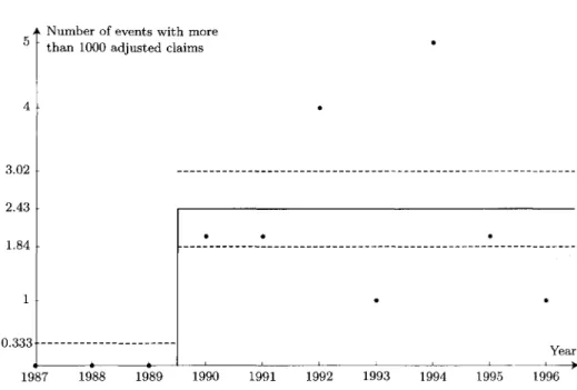
Figure 4.1 contains an illustration of the counting data and this empirical mean. Since Var(jVy) = A, the variance of the estimator Xf^ in (4.2) is X/n
- i const
MOOO
1 \J\J\J
with n = 10, hence the estimated standard deviation of Awi™ is
It remains to determine the probability that an event, which causes more than 1 000 adjusted claims, actually causes at least 6000 adjusted claims and therefore leads to the knock-out of the corresponding WINCAT coupon. For
this purpose we shall consider a sequence {Xk}keN of independent,
identically distributed random variables, where A* describes the severity of the kth event. We always assume that the sequence {X/(}keN is independent of
7V1987, ..., Ni996- The random variables X\, ..., XNmi are used to describe
the severity of the events in 1987, the variables XNmi+\, ..., Xivmi+Nmx those
in 1988 and so on. In the following subsections we consider three different distributions for the random variables { X ^ ^ .
A Number of events with more than 1000 adjusted claims
2.11 1.7 1.29 1 Year 1987 1988 1989 1990 1991 1992 1993 1994 1995 1996 FIGURE 4.1: Observed number of events in the ten observation periods November 1st to October 31st causing more than 1 000 adjusted claims. The empirical mean of A"^' = 1.7 events per observation period is also shown. The dashed lines indicate the estimated standard deviation 0.41 of the estimator A'jJJJJ given
by (4.4). The estimated standard deviation for the distribution of the observations is
4.1. Bernoulli distribution for the knock-out events
In this subsection we introduce a simple model to describe events with more than 1 000 adjusted claims, which actually cause at least 6 000 adjusted claims; meaning that they lead to a knock-out of the WINCAT coupon. For this purpose we introduce Bernoulli random variables X\, ..., Xm for the
m — 17 events, where Xk = 1 means that event number k e {1, ..., m)
caused at least 6 000 adjusted claims. We set Xk = 0 otherwise. We assume that Xy, ..., Xm are independent and identically distributed. Proceeding as in
Section 3, we can estimate the probability /?6ooo = P(^/t = 1) by the unbiased empirical mean
£ * (4.5)
m k=\
The data of Table 1.1 leads to /?6ooo = 2/AW = 2/17 «0.118. An analysis similar to (3.2) and (3.3) gives the estimate
114 UWE SCHMOCK
If N is a random variable with the Poisson distribution given by (4.1) describing the number of events, and if independently of everything else we perform a Bernoulli experiment with success probability peooo £ [0,1] for each of the TV events, then an elementary exercise shows that the resulting number of successful events has a Poisson distribution with parameter /?6oooA. Therefore, under the above assumptions, the number of events per observation period leading to at least 6000 adjusted claims has a Poisson distribution. An estimate for the corresponding Poisson parameter is
•vconst ~ \ c o n s t (\ ~> IA 1\
A
6000 = ^6000 • A1000 = — • — = — = 0.2 . (4. /)
The probability that no such event happens, is given by exp(—Ag^4), see (4.1) with k = 0. Hence, the estimated knock-out probability is
PCAT = 1 - e x p ( - A ^ ) = 1 - exp(-0.2) « 0.181 . (4.8)
A recalculation of Table 3.2 with this value of PQKJ leads to a discounted value of CHF 249.93 for the three WINCAT coupons.
To estimate the knock-out probability of the first WINCAT coupon, we have to replace A ^ f = 17/10 from (4.3) by A'j^o =15/10, because only 15 events are recorded in Table 1.1 for the period from February 28th to October 31st. This leads via (4.7) and (4.8) to
( 4 9 )
which is exactly the same result as the one obtained by applying the correction formula (2.1) to the result of (4.8).
The variance of the estimator A^jf is not easily computable from the variances of j?6ooo and AJQQQ*, because these two estimators are dependent (knowing A^jf restricts the set of possible values for^ooo)- According to our model assumptions however, we have observations from n = 10 independent Poisson random variables available, which describe the number of events in each of the ten observation periods leading to at least 6 000 adjusted claims. Similar to (4.2) and (4.4), we therefore see that the estimator (4.7) for Ag^jf is unbiased and that
For a conservative estimate of the knock-out probability we might use
/>CAT = 1 - e x p ( - A ^ - ( T ( A ^ ) ) « 1 - exp(-0.341) « 0.289 . A recalculation of Table 3.2 with this value of PCAT leads to CHF 218.24 for
There is a methodical problem with the approach in this subsection so far. We are mainly interested in an unbiased estimator for the knock-out probability PCAT- The unbiasedness of the estimator A^QQ* for a model specific parameter is not of primary concern. To elaborate on this point, let •/V6ooo,« be t n e n u mb e r of events with at least 6 000 adjusted claims within
n = 10 observation periods. According to our model assumptions, A^6ooo,«
has a Poisson distribution with parameter np\, where A is the intensity for the number of events per observation period with more than 1 000 adjusted claims, and/? = />6000 is the "success" probability for the following Bernoulli experiment indicating whether actually at least 6000 adjusted claims arise from the event. The estimator (4.8) corresponds to
PCAT = 1 - exp(-JV6Ooo,«/«) (4.10) with n = 10. Calculating the expectation gives
- exp(-AW>,«/«)] = 1 - Y
te-klH
^£
Le-
mpX k=0 oo ~ 2-~i k} = 1 — exp (—(1 — e~l/")np\),which is different from 1 — exp(—p\), hence (4.10) is biased. Multiplying o,n in (4.10) by the correction factor log MM" leads to the estimator
(
1 \ #6000,n1 - - J (4.12)
with expectation 1 — exp(—p\) as a calculation similar to (4.11) shows. Hence the estimator (4.12) is unbiased. Since n = 10 and A^ooo.io = 2 by Table 1.1, we obtain
The corresponding recalculation of Table 3.2 gives C H F 247.37 for the discounted value of the three WINCAT coupons.
For the variance of the estimator in (4.12) we obtain after a short calculation similar to (4.11)
Var(PCAT) = E
1-i
n2^6000.™
Using the estimate \<$$ = 0.2 for pX from (4.7) and (9/10)2 for e-pX from (4.13), we obtain
/ (^\ 0.115 . (4.14)
A recalculation of Table 3.2 with the conservative knock-out probability
^CAT + ^(^CAT) ~ 0.305 gives C H F 213.73 for the discounted value of the WINCAT coupons.
The estimated standard deviation in (4.14) is slightly smaller than the one in the simple binomial model calculated via (3.3). This indicates that in our case the composite Poisson model of this subsection leads only to a slight improvement. Indeed, the estimator (4.13) for the knock-out probability uses only the information that two events within the ten years caused at least 6000 adjusted claims. Since the model of this subsection allows these two events to happen in the same year, the estimated knock-out probability in (4.13) is 1% lower than the one in the binomial model. If the two events with at least 6000 adjusted claims had actually happened in the same year and not in consecutive ones, the discrepancy in the estimated knock-out probabilities would be 9%, because the estimate in the binomial model of Section 3 would drop from 20% to 10%. In this respect the composite Poisson model of this subsection is more robust than the binomial one.
4.2. Pareto distribution for the knock-out events
The binomial model of Section 3 and the corresponding composite Poisson model of Subsection 4.1 do not use the adjusted claim numbers recorded in Table 1.1. For the benefit of a better estimate of pawo, let us incorporate these numbers into the model. The step function in Figure 4.2 is the empirical distribution function of the adjusted claim numbers from Table 1.1. A heavy-tailed distribution of common use is the Pareto distribution, its distribution function is given by
. , \\-(a/x)h for x > a, , , , ^ Pareto^ (x) = { V ' ' " (4.15)
^ 0 for x < a,
where a and b are strictly positive parameters. The Pareto distribution is used in [3] to model the number of adjusted claims per event given that more than 1 000 adjusted claims arise from the event. We choose the threshold
a = 1000, because only such events are contained in Table 1.1. At first glance
it might look as if we make a conceptual mistake by fitting the distribution of an apparently integer-valued random variable by a distribution having a density. However, the involved numbers from the last column of Table 1.1 are sufficiently large for such an approximation and, in addition, they are actually rounded numbers arising as the product of the number of claims
and the vehicles insured index. Therefore, the use of a continuous distribution function should not cause an intellectual problem (see Section 6 and the end of Section 13 however).
To fit the empirical distribution with a Pareto distribution as in Figure 4.2, we need an estimator for the exponent b. If a random variable X has a Pareto distribution with parameters a and b, then Y = log(X/a) satisfies
P( Y < y) = P(X < aey) = 1 - ( - ^ ) = 1 - e~by, y > 0,
which means that Y has an exponential distribution with expectation
E[Y] = \/b. Hence, if the independent random variables X\, ..., Xm, with a
Pareto distribution given by (4.15) describe the adjusted number of claims for the m events, then the random variables Y\, ..., Ym with Yk = \og(Xk/a)
are independent and exponentially distributed. Their empirical mean 0 /w) Z X - i Yk is an unbiased estimator for \jb. This suggests to estimate
b by the reciprocal value
k=\ Yk L,k=
Another way to derive this estimator is to consider the likelihood function
h
which is the product of the densities of the Pareto distribution (4.15) evaluated at X\, ..., Xm. By differentiating the logarithm of Lm, we find that
b given by (4.16) maximises Lm, hence (4.16) is also the maximum-likelihood
estimator for b.
Let us calculate the expectation of the estimator in (4.16). The sum
YTk-\ Yk has a gamma distribution with parameters m and b, meaning that
This fact is easily proved by an induction on m, because the convolution of the exponential density and the gamma density of parameter m leads to the gamma density of parameter m + 1:
)m-xe-bsds = ^{bt)me-b
(bs)m-xe-bsds = ~^-~{bt)me-b\ t > 0, mT{m)
118 UWE SCHMOCK
Number of adjusted claims
0.2 •
2000 4000 6000 8000 10000 12000
FIGURE 4.2: The step function is the empirical distribution of the number of (adjusted) claims per event, given that more than 1 000 claims arise from the event. Also shown is the fitted Pareto distribution (4.15) with
a = 1000 and b = bn, where bn ss 1.37 is the maximum-likelihood estimate, corrected with the factor (m — \)/m for m = 17 to eliminate the bias. The estimated probability, that an event with at least I 000 claims
causes at most 6000 claims, is around 0.914. Two additional Pareto distributions (dashed curves) illustrate the estimated standard deviation of An- The lowed dashed curve corresponds to bn — &(f>n) « 1.02, the
upper one to bn + a(bn) sa 1.73.
and the gamma function satisfies T(m + 1) = mT(m). Calculating the expectation of (4.16) for m > 2 shows that
m
-1 =
f-la)\ Jo t
mb Z"00 b{bt)m-2e-htdt = m
(4.18)
m — 1-b.
This means that the estimator in (4.16) underestimates the tail of the Pareto distribution. To obtain an unbiased estimator for b, we therefore have to use
bm —
m — 1
(4.19) instead of (4.16). The data from the last column of Table 1.1 leads to
bn w 1.37 . (4.20)
A calculation similar to (4.18) leads to
V a r ( f tm) =/^ (4.21) for all m > 3. Therefore, a(bm) — bmj\/m — 2 is an unbiased estimator for
the standard deviation; using the numerical value from (4.20) gives
< T ( &1 7) « 1 . 3 7 / V 1 5 « 0 . 3 5 . (4.22)
The Pareto distributions with b\7 ± &(b\7) are shown as dashed curves in
Figure 4.2.
Using bm for the parameter of the Pareto distribution (4.15), we obtain
the estimator
Peoao = 1 - ParetoloooAii(6000) = ^h"' (4.23) for the probability that an event, which causes more than 1 000 adjusted claims, actually causes at least 6000 adjusted claims. The numerical value
bxl K, 1.37 from (4.20) leads to
Peooo « 6 -L 3 7« 0.0857. (4.24) Considering the two Pareto distributions corresponding to b\j — cf(bn) « 1.02 and b]7 + a(bv) « 1.73 (see Figure 4.2), we obtain via (4.23) the
asymmetric interval
j ^ [0 0 4 5 ) 0 1 6 2] (425) around the estimate /?6ooo ~ 0.0857 as an indication of the standard deviation. This is an improvement compared to the interval [0.037, 0.199] arising from the Bernoulli distribution via (4.6).
F'ollowing the approach in [3], we recalculate the estimate (4.7) for the Poisson parameter A^JJjf describing the number of knock-out events per observation period using A'JQJJQ1 = 1.7 from (4.3) and peooo ~ 0.0857 from (4.24). We obtain A ' ^ = pm(l • X^f « 0.1457. As in (4.8), the estimated
knock-out probability is
PCAT = 1 - c x p ( - A ^ ) = 1 - exp(-A,ooo • XTm) « ° -1 3 5 6 • (4-26)
A recalculation of Table 3.2 with this value of PcAT leads to a discounted value of CHF 263.29 for the three WINCAT coupons.
To get a rough estimate of the standard deviation of the knock-out probability in (4.26), consider it as a function of the two parameters b\7 ^n A \ — \ const.
a n d A = Al 0 0 0 .
Using the approximating plane in (b, A) and thereby neglecting all higher order terms in the Taylor expansion, we get
Since b\-j and A are unbiased, we obtain for the variance
> i 7 ) + ( — ^ ( M ) ) Var(A)
The two estimators bm and A = Xc°^ are certainly not independent,
because the observed number m of events determines A " ^ via (4.3) and the variance of bm via (4.21). However, b\j and A are independent and
therefore uncorrelated, meaning that E[(S]7 - b)( A - A)]. Evaluating the partial derivatives of the knock-out probability PcAr at the
estimated point (bn, A) instead of (b,X), and using the estimated standard deviations from (4.22) and (4.4) instead of (Var(6,7))1/2 and (Var( A))1/2, we obtain the approximation
\ "X )
w 0.086. (4.27) From (4.26) and (4.27) we obtain PCAT(^17, A) + a(PCAT{b]7, A)) w 0.221
as a conservative estimate of the knock-out probability. A recalculation of Table 3.2 leads to a discounted value of C H F 238.25 for the three WINCAT
coupons. Due to these calculations, in [3] the rounded knock-out probability of 0.25 is considered to be a conservative estimate, leading to a discounted value of CHF 229.78. ' This value is supposed to include a risk premium for the investor because the standard deviation of the knock-out probability is added and the result rounded in a conservative way.
Before turning our attention to a generalised Pareto distribution for the knock-out events, let us conclude this subsection with some supple-mentary considerations concerning the biasedness of the estimators for />6ooo and PCAT- First note that A^Q* from (4.2) and bn from (4.19) are unbiased estimators for the two model parameters A and b, but this does
' In [3] a discounted value of CHF 227.09 is actually derived, because the 15/17-corrcction for the first observation period is not taken into account.
not imply that /?6ooo and PCAT, given by (4.23) and (4.26), respectively, are unbiased. The arguments leading to the unbiased estimator (4.12) in the case of the Bernoulli distribution for the knock-out probability in Subsection 4.1 suggest that the estimator
/ £>AAAn\ ^VlOOO.d / 6 l 7
\ ^1000,(1
PCAT
= \-[\ - ^ ) = 1 - ( l — ) (4.28)
is a small improvement, because this would be an unbiased estimator for
PCAT if bn were non-random. Here the random variable Mooo,« denotes the number of events with more than 1000 adjusted claims within the n observation periods. Recall that Mooo,« has a Poisson distribution with parameter n\. Substituting our estimate bn « 1.37 from (4.20) and Wiooo,n = 17 for the n = 10 observation periods into (4.28) leads to
AJAT ~ 0.1361, which gives a discounted value of C H F 263.13 for the three
WINCAT coupons. This is a decrease of only C H F 0.16 compared to the value
arising from (4.26).
If we consider #1000,10 = 17 as non-random and replace bn « 1.37 from (4.20) by bn — &{b\q) ss 1.02 in the estimator (4.28) to find a conservative estimate, we get PC A T ~ 0.242, which via Table 3.2 leads to C H F 232.14 for
the discounted value of the three WINCAT coupons. Note that this knock-out probability is abknock-out 0.02 larger than the one obtained from (4.27) and is already very close to the conservatively rounded value of 0.25 from [3].
An examination of the above model reveals that the conditional distribution of the estimator bm given m = JVIOOO,« is only specified in
the case A^iooo.n > 2. Furthermore, (4.21) shows that bm does not have a
variance unless m = JVIOOO.M > 3. Hence, the above approach of fitting the empirical distribution of the adjusted claim numbers by a Pareto distribution is applicable only in the case of appropriate data sets. Such an a priori exclusion of certain data sets already introduces a bias which suggests that unbiasedness for estimators like (4.26) or (4.28) is a problematical notion. Maybe a notion of conditional unbiasedness would be more appropriate. This means in our case that one would like to have estimators for PCKT such
that the conditional expectation given />6OOO#IOOO,H > 1, for example, is the right one.
4.3. Generalised Pareto distribution for the knock-out events
In Subsection 4.2, we did not give a theoretical argument in favour of the Pareto distribution in addition to the desire to pick a heavy-tailed distribution. Let us use an idea from extreme value theory to overcome this deficiency. It will turn out that we should use a generalised version of the
Let X\, ..., Xk denote the adjusted number of claims arising from k events. We shall assume that X], ..., X^ are independent and distributed according to a heavy-tailed distribution function. We are only interested in those numbers which exceed a certain threshold a, which is 1 000 in our case. This means we are interested in the excess distribution function
Fa(x) = P(X] -a<x\X\> a), x£R.
Extreme value theory essentially says the following in our case [6, Section 3.4]: If the original distribution function of X\, ..., X^ is heavy-tailed, then the excess distribution functions {Fa}a>o can be better and better
approximated (with respect to the supremum norm) by generalised Pareto distributions of the form
for x > 0, for x < 0,
as the threshold a tends to infinity. Here £ is a strictly positive ' shape parameter and the scale parameter ra > 0 varies with the threshold a. This
suggests that we should try to fit the empirical distribution function of the observations exceeding the threshold a by a distribution function of the form
<w*> = (!-
( 1 +
*^
) / r r
T-"'
(4
-
29)
[0 for x < a.
Note that in the heavy-tailed case £ > 0, the (shifted) generalised Pareto distribution (4.29) with r = a£ reduces to the Pareto distribution (4.15) with b = l/£. Hence, Ga^T gives us the freedom of the additional scale
parameter r.
Before fitting a generalised Pareto distribution function to the observa-tions, an exploratory data analysis should be done, see [6, Chapter 6], to check the assumption of a heavy-tailed distribution and to determine a suitable threshold. However, since there are only m = 17 observations available in Table 1.1, there seems to be no point in choosing a higher threshold than a = 1 000 in our case, because the historical data set is quite small already. The assumption of a heavy tail is (at least partially) supported by Figure 4.4.
The log-likelihood function for the m = 17 observations originating from a generalised Pareto distribution is
l + T j I ^ l o g f l + e ^ ). £>0,r>0. (4.30)
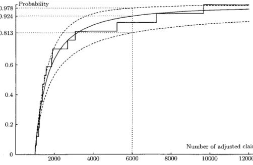
0.978 r Probability
Number of adjusted claims
2000 4000 6000 8000 10000 12000
FIGURE 4.3: The empirical distribution of the number of adjusted claims per event (solid step function) and the fitted generalised Pareto distribution (solid curve) with threshold a = 1 000, estimated exponent l/£ ss 1.38 and estimated scale parameter f ss 660.7. The estimated probability that an event with at least 1 000 claims causes at most 6000 claims, is approximately 0.924, and [0.813, 0.978] is an approximate
68%-confidence interval for this probability. The two dashed curves are generalised Pareto distributions chosen such that they indicate the standard deviation of the estimated probability for at most 6000 claims.
Inserting the data from the last column of Table 1.1, we can calculate the maximum-likelihood estimator (£, f) numerically, i.e., we can search for the point (|, f) which maximises /. As starting values for the numerical iteration procedure, we can choose £ = \/bm and r = a/bm, where bm is the estimator
(4.19) for the Pareto distribution, or we can use a probability-weighted moment approach (see [6, Section 6.3.2 and page 358]) to obtain a priori estimates for £ and T. We find
0.7243 and f » 660.7, (4.31)
hence
/>6ooo = 1 - Gmolf(6000) « 1 - 0.92425 = 0.07575. (4.32)
The corresponding fit of the empirical distribution with a generalised Pareto one is shown in Figures 4.3 and 4.4. A calculation as in (4.28) gives the estimate
1 - 0.121,
124 UWE SCHMOCK 1000 1 0.7 0.5 0.3 0.187 0.15 0.1 0.076 0.05 0.03 0.022 i Tail probability
**Sti on logarithmic scale
^ ^ ~-~--~.
> 1500 2000 2500 3000 4000 5000 6000 7000 9000
Number of adjusted claims on logarithmic scale
FIGURE 4.4: This is Figure 4.3 on log-log scale to magnify the important part. Instead of the distribution functions, the corresponding tail probabilities are shown. Pareto distribution functions defined by (4.15) would give straight lines in this log-log plot. The estimated generalised-Pareto fit jr i—>• 1 — Gnmrr{x) 's close
to a straight line because a£/f ss 1.096 is quite close to one. The estimates plmn ~ 0.022, p(m> ~ 0.0757 and
Pum ~ 0.187 are shown. This figure supports the model assumption, that the adjusted claim numbers follow
a heavy-tailed distribution.
For comparison with the earlier results on the standard deviation of /?6ooo in the case of the Bernoulli distribution for the knock-out events in (4.6) and for the corresponding case of the Pareto distribution in (4.25), we would like to give again an estimate for the standard deviation of pmo- This does not seem to be possible by analytical means, however. Therefore, we prefer to construct ah interval [^60001^6000] a r o u nd the estimated value />6ooo ~ 0.0757 from (4.32), which can serve as the region for accepting the null hypothesis
P = P6000 at a 68%-confidence level when using the log-likelihood ratio
statistic. We choose the 68% level, because this is the probability that a normally distributed random variable with mean fi and variance a2 > 0 takes its value in the interval [/J — a, /x + a]. As log-likelihood ratio statistic, also called deviance, we use
, T) = 21(1 T) - 2/(£, T), £ > 0, r > 0. (4.33)
We want to determine the smallest interval [/>6~ooo>/'600o] s u c n t n a t
c
G (0,CX)) 1 - G,ooo^.r(6OOO) G [/W/>6+ooowhere X2032 ~ 2-30 denotes the 32%-quantile of the chi-squared distribu-tion with two degrees of freedom. In other words: We are looking for the smallest probability P^QQ and the largest probability / ^0 0, which can arise from generalised Pareto distributions with parameters (£, r) close to (£, f) in the sense that the deviance Z>(£, r) does not exceed the 32%-quantile xlo.32 of the x^-distribution. This choice for the upper bound of the deviance
D(£, r) is based on the asymptotic normality of the maximum-likelihood
estimators, see for example [10, Section 8.8]. According to [12, Appendix A], the approximation of the distribution of the deviance by the chi-squared distribution is often quite accurate for small numbers of observations, even when the normal approximation for the parameter estimates is unsatisfac-tory. When compared to methods using the second derivatives of the log-likelihood function at the estimated point (£, f), the log-log-likelihood ratio statistic has the advantage of being able to give asymmetric confidence intervals and thereby being less prejudiced. This is useful in our case, because we don't want to obtain negative estimates for p^000, for example. It should
be kept in mind that (4.34) is in general a strict inclusion, hence [p6ooo'i'6ooo] can correspond to a higher confidence level than 68%. This is problematical for larger numbers of parameters, because the confidence intervals get too large. Bootstrap methods are an alternative in this case.
Note that the interval [P6ooO'^60oo] m (4-34) does not depend on the parametrisation arising from (|, r) 1—> GIOOO,£,T in (4.29). We can use this
observation to change to an advantageous parametrisation which reduces the amount of numerical calculations necessary to determine the above acceptance interval. Since the equation/? = 1 — Giooo,(,r(6000) can be solved for r yielding
5000C
T(£P)
we can use/> itself as a parameter by changing the parametrisation from (4.29) to (£,/?) H-> GIOOO,£,T(£,/>). Rewriting the inclusion (4.34) with this parametrisation yields {(£,/>) € (0,oo) x (0,1) | Z>(£r(£,/>)) <X2,O.32> C (O. ° ° ) X [PMOO A O ]
-Numerical calculations lead to [P6ooo>/\tooo] ~ [0-022, 0.187], the correspond-ing exponents |~ « 0.355772 and | + « 1.396 are the only ones with a deviance less or equal to the quantile X2 0 32- The shifted generalised-Pareto distribution functions x •-> Giooo,c ,f W w i t h r = T{ir,Pmo) ~ 6 2 0-3 and x » Gim4-f> (x) w i t h f+ = T{£+>Ptooo) « 7 4 0-6
are shown in Figures 4.3 and 4.4. If we consider the number /Viooo.io = 17 as non-random and use /^000 ~ 0.187 instead of peom, a calculation as in (4.28) leads to the conservative estimate PCAT ~ 0.274. A recalculation of Table 3.2 gives a discounted value of C H F 222.75 for the three WINCAT
coupons.
5. TESTING THE CONSTANT-PARAMETER POISSON MODEL
5.1. Testing for over-dispersion
In Section 4 the number of events with at least 1 000 adjusted claims per observation period is modelled by ten independent random variables Ny for
the years ^ G { 1 9 8 7 , ..., 1996}, each one having the same Poisson
distribution (4.1) with parameter A > 0. Since the expectation and the variance of the Poisson distribution are equal to the parameter A, the empirical mean \c°^ of 7V"i987, •••, -^1996 was used in (4.2) as an unbiased
estimator for the expectation and the variance. However, if we don't want to rely on the assumption of a Poisson distribution when investigating the variance (but keep the assumption that N\9$j, ..., /V1996 are independent and identically distributed), then we should estimate the variance a2N — Yar(Ny)
by the unbiased estimator
, 1996 , 1996
4 E ^
q w i t hM*
ith^
j=1987 >>=1987
The data of Table 1.1 leads to &2N = 2.9, which yields the standard deviation
a(fcN) = ^Ja2N/10 = A / 2 9 / 1 0 « 0.54 (5.1)
for the empirical mean (iff of Nmj, ..., Nigg^. Note that a2N = 2.9 is quite a
bit larger than Xf^f = 1.7 from (4.3). This observation raises the question whether the data of Table 1.1 exhibits over-dispersion, meaning in our case that the variance of /V1987, ..., iVi996 is actually larger than the mean. Such an over-dispersion can arise, for example, from a Poisson parameter A which is itself a random variable. In the present case, global weather conditions could have determined different values for A in the ten observation periods. See, e.g., [12] for a discussion of over-dispersion.
To investigate this question of over-dispersion, let us consider the possibility that a large variance as above, namely &2N > 2.9, happened by
chance. This means that we want to calculate the conditional probability
V[&2N > 2.9 I (iff = 1.7) under the null hypothesis that A^i987, •••, ^1996 are
independent and distributed according to (4.1) with an unknown Poisson parameter A > 0. The small number of observations and their small values make it feasible to calculate the above conditional probability exactly.
Under the null hypothesis, the sum iVi987 + •••+ M996 has a Poisson distribution with parameter 10A and we obtain
F(Ny = ny for every y e {1987, ..., 1996} | £LN = 1.7) X
\A /(
1 O A)
1 7iZL ft J (
5-
2)
for every t u p l e («i987, •••, «i996) €E NQ° with «i9 87 + ... + 721996 = 17. N o t e t h a t
the conditional probability in (5.2) does not depend on the unknown parameter A > 0. For every tuple in (5.2), there are
10!
- .
1 9 9 6)
w i t h ny = 0 )
!different rearrangements of the tuple; all of these lead to the same probability in (5.2). A small program, ' which considers all possible tuples for (5.2) satisfying ny+x <ny for all ye {1987, ..., 1995}, finds 267 such
tuples and yields
> 2.9 I /ijv = 1.7) « 0.0889 . (5.3)
(a N >
While this one-sided test does not show a significant deviation from the Poisson distribution on the 5%-level, it is certainly more conservative to use the standard deviation a(p,N) « 0.54 from (5.1) instead of o^A^o*) ~ 0.41
from (4.4) to take the possibility of over-dispersion into account. Combining this result with the fitted Pareto distribution for the knock-out events (see Subsection 4.2), the analogue of (4.27) for the approximation of the standard deviation of the knock-out probability gives (r(Pc£r(bn, A)) « 0.0893. Together with (4.26) we obtain PCAT(6, A) + (T(PCAT(^, A))« 0.225 as a
con-servative estimate of the knock-out probability. A recalculation of Table 3.2 leads to a conservative discounted value of C H F 237.15 for the three WINCAT
coupons. This is only CHF 1.10 below the conservative value CHF 238.25 derived from (4.27).
It is possible to test the assumption of a Poisson distribution further by choosing an explicit alternative like a negative binomial distribution and considering the corresponding Neyman-Pearson test. In addition, we could choose a preferred measure of discrepancy for distributions and apply model selection criteria to come to a decision about the underlying distribution. In this paper, however, we want to pursue a different route, namely a possible deterministic time-inhomogeneity of the distribution of the numbers 7Vi987, ..., Ni996 of events per observation period. Concerning model selection in the case of independent and identically distributed random
The Mathematka command NumberOfPartitions! 17] from the standard add-on package DiscreteMath'Combinatorica" shows that there are 297 partitions of 17 altogether, hence the running time of the program will be acceptable. Unnecessary loops in the program can be avoided
variables, we therefore refer the reader to [11], in particular to [11, Example 4.4.3], where the Poisson and the negative binomial distribution are the alternatives.
5.2. Testing for time-inhomogeneity
When looking at Figure 4.1 which shows the number of events in the ten observation periods causing more than 1 000 claims, we can ask whether there is something special about the order of the ten observations; in particular, whether the assumption of an identical distribution for the random variables Nmj, ..., N\w(, is justified.
Starting from (0, 0, 0, 1, 1, 2, 2, 2, 4, 5), namely the ten observations in increasing order, we need 38 successive transpositions of adjacent entries of the tuple to rearrange it in decreasing order. To rearrange the observed tuple (0, 0, 0, 2, 2, 4, 1, 5, 2, 1) into decreasing order, we need 28 successive transpositions of adjacent entries:
(0,0,0,2,2,4,1,5,2,1) —»• (2,2,4,1,5,2,1,0,0,0) 21 transpositions -> (2,2,4,5,2,1,1,0,0,0) 2 transpositions -+(4,5,2,2,2,1,1,0,0,0) 4 transpositions -> (5,4,2,2,2,1,1,0,0,0) 1 transposition
Since the number of 28 transpositions is well above the half of 38, we can use this observation for a permutation test to find out whether the data shows a tendency to be arranged in increasing order.
Under the assumption that the ten observations are given by ten exchangeable, No-valued random variables N1987, ..., N1996 every permuta-tion of the ten observapermuta-tions has the same probability. If N\g^, ..., N\g% are independent and identically distributed, then exchangeability follows. For every one of the
37312! =
5°
4 0°
(5'
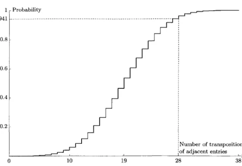
5) different permutations of the ten observations, we can count the required number of successive transpositions of adjacent entries to obtain the decreasing order given by the tuple (5, 4, 2, 2, 2, 1, 1, 0, 0, 0). This number is always between zero and 38. Figure 5.1 shows the resulting distribution function of this number.Under the null hypothesis where all permutations of the ten observations have the same probability, only for 2 953 permutations out of 50 400, about 5.86% of them, 28 or more transpositions of adjacent entries are needed to reach the decreasingly ordered tuple. (If there were a substantially higher number of permutations than 50400, then a suitable number of random permutations would have to be generated in order to get an estimate for this percentage.)
1 p Probability 0.941 —
Number of transpositions of adjacent entries
0 10 19 28 38
FIGURE 5.1: Distribution function of the number of successive transpositions of adjacent entries necessary to order a random permutation of the ten observations into decreasing order. For the observed data, 28 transpositions are necessary. At least 28 transpositions are necessary for about 5.86% of all permutations.
Note that for the permutation test of this subsection we do not assume that the distribution of Nw, ••-, N1996 lies in a certain class; in particular, the test is parameter-free. Furthermore, the test does not depend on the actual numbers but merely on their relative order or ranks; an observation like (0, 0, 0, 3, 3, 4, 1, 7, 3, 1) would give the same test result. For such a distribution-free test and just ten observations, 5.86% is a remarkable result. However, as we can see from (5.4), it is mainly caused by the position of the three zero observations.
6. FITTING A GENERALISED EXTREME VALUE DISTRIBUTION
For a knock-out of a WINCAT coupon, only the most severe event within
the corresponding observation period matters. We can use extreme value theory to model this event directly. The theoretical background for this approach is the Fisher-Tippett theorem (see for example [6, Theorem 3.2.3]), which identifies all possible limit distributions for properly scaled maxima M(n) = max{X\, ..., Xn} of independent, identically distributed
random variables X\, ..., Xn as n —> 00. If the distributions of the properly
scaled maxima do converge, then the limiting distribution is either a Frechet, a Weibull or a Gumbel distribution. In the following we use the Jenkinson-von Mises representation of these extreme value distributions,
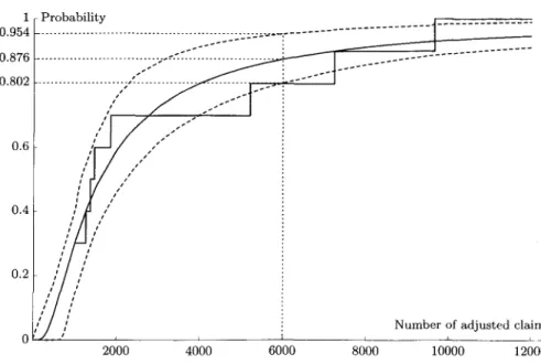
130 UWE SCHMOCK r Probability
Number of adjusted claims
2000 4000 6000 8000 10000 12000
FIGURE 6.1: The censored empirical distribution function of the number of adjusted claims of the most severe event per year (solid step function) and the fitted generalised extreme value distribution (solid curve) with estimated exponent l/£ « 1.316, scale parameter f as 1008 and location parameter /"/, ss 1168. The estimated probability, that no knock-out event occurs within one year, is approximately 0.876. The two dashed curves, derived from 1 000 bootstrap samples, indicate 68%-confidence intervals for the fitted generalised extreme
value distribution.
the scale parameter and £ e M. the shape parameter. In the case £ > 0, which corresponds to the Frechet distribution, we define the distribution function
Hn,(,T by
r'/
£), if l + £ ( j f - / i ) / T > 0 ,
otherwise.
In the case £ < 0, which corresponds to the Weibull distribution, we define
similarly
otherwise.
With the above representation, the Gumbel distribution
HpflAx) ~ exp(—exp(-
(x-for the case £ = 0 is actually the limit of H^T as £ —> 0.
When fitting the generalised extreme value distribution with /x, £ € R and r > 0 to the observed maxima given in Table 1.1, we have to
cope censored data. The most severe events of the years 1987-1989 are not given because they caused less than 1 000 adjusted claims (assuming that there were damages caused by storm or hail at all). Next, when we want to use the maximum-likelihood method to estimate the parameters /x, £ and r, we encounter another problem: The density of H^T is unbounded for
£ < - 1 and
x /
fi-
T/\.Both problems can be solved by discretizing the distribution H^^j. The censored data for the years 1987-1989 corresponds to three observations in the interval (0, 1000]. The most severe events in the years 1990-1996 are adjusted claim numbers which correspond to intervals of the form (n, n + 1] with an integer n > 1000 (at least approximately, ignoring that the vehicles insured index in Table 1.1 is not always exactly one). This suggests the likelihood function
1996
3
j=1990
with ( i , ( e R and r > 0, where M1990, ..., M1996 denote the yearly maxima from Table 1.1. The numerical iteration procedure applied to the log-likelihood function leads to the maximum-log-likelihood estimates /t w 1168, £ « 0.760 and f « 1008; the corresponding fit is shown in Figure 6.1. These values lead to an estimated knock-out probability of only
PCAT = 1 - 77/^^(6000) « 12.4%, because the fitted distribution is well
above the empirical one at 6 000 in Figure 6.1. A recalculation of Table 3.2 gives a discounted value of C H F 266.62 for the three WINCAT coupons.
For further background on parameter estimation for the generalised extreme value distribution, see [6, Section 6.3] and the references given there.
It would be unreasonable to insist on estimates for \x, £ and r giving a generalised extreme value distribution with support in [0,00), because
Hfi,li(0) « 6.8 • 10~8 is already a very good approximation of zero, the true distribution is almost certainly not in the family {H^T | ju,£ <E R, r > 0},
and a good fit at this end of the distribution, where the data is censored anyway, is not our primary concern.
To estimate the 68.3%-confidence intervals in Figure 6.1, we use the bootstrap method; see e.g. [5] for an introduction. We take 1 000 bootstrap samples (Mjf987, ..., Mf996), where for each component the values M1990, ..., M1996 have probability 1/10 of being chosen, and with probability 3/10 we take a censored observation. For each bootstrap sample we calculate the corresponding maximum-likelihood estimate (/}*, £*, f *). This gives 1 000 bootstrap values for H^^^^x), we take the 159th and the 841st largest values as boundaries for a 68.3 %-confidence interval for H^lf{x). The estimated 68.3 %-confidence interval for the above knock-out probability is [0.046, 0.198]; the conservative estimate PCAT = 0.198 leads to a discounted