Tests of structural changes in conditional distributions with unknown changepoints

HAL Id: halshs-00611932

https://halshs.archives-ouvertes.fr/halshs-00611932

Submitted on 27 Jul 2011

HAL is a multi-disciplinary open access

archive for the deposit and dissemination of

sci-entific research documents, whether they are

pub-lished or not. The documents may come from

teaching and research institutions in France or

L’archive ouverte pluridisciplinaire HAL, est

destinée au dépôt et à la diffusion de documents

scientifiques de niveau recherche, publiés ou non,

émanant des établissements d’enseignement et de

recherche français ou étrangers, des laboratoires

Tests of structural changes in conditional distributions

with unknown changepoints

Dominique Guegan, Philippe de Peretti

To cite this version:

Dominique Guegan, Philippe de Peretti. Tests of structural changes in conditional distributions with

unknown changepoints. 2011. �halshs-00611932�

Documents de Travail du

Centre d’Economie de la Sorbonne

Tests of Structural Changes in Conditional Distributions

with Unknown Changepoints

Dominique G

Philippe de P

Tests of Structural Changes in Conditional

Distributions with Unknown Changepoints

Dominique Guégan

Philippe de Peretti

July 18, 2011

Abstract

This paper focuses on a procedure to test for structural changes in the …rst two moments of a time series, when no information about the process driving the breaks is available. To approximate the process, an orthogonal Bernstein polynomial is used, and testing for the null is achieved either by using an AICu information criterion, or a restriction test. The procedure covers both the pure discrete structural change and the continuous changes models. Running Monte-Carlo simulations, we show that the test has power against various alternatives.

Keywords: Structural Changes ; Bernstein polynomial ; AICu

1

Introduction

This paper deals with models of the form:

A(L)yt= ct (1)

where: A(L) = 1 ₁L ₂L2 _:::

pLp;

ct is either de…ned as ct= f (t) + "tor ct= f (t)"t, where in both cases f (t) is

Université Paris1 Panthéon-Sorbonne, 106-112 Bd de l’Hôpital, 75013 Paris, France. [email protected]

y_{Université Paris1 Panthéon-Sorbonne, 106-112 Bd de l’Hôpital, 75013 Paris, France.} [email protected]

an unknown, possibly time-varying signal, thus inducing heterogeneity in one of the two moments of the conditional distribution, "tis an iid term.

For instance, assume the simple case where f (t) is de…ned as a step-function for the mean: f (t) = 8 < : 1 if t t0 2; otherwise (2) with 16= 2and t02 ( 1T; T (1 2)):

Perron (2005) stresses the importance of testing for structural changes. On the one hand, structural changes are a source of global non-stationarity (Granger and Starica [2005], Guégan [2010]) and then of parameter instability, and on the other hand, ignoring structural changes may lead to erroneous statistical infer-ence in tests for stationarity (Perron [1989]), and for long memory (Diebold and Inoue [2001], Char¤edine and Guégan [2011]). Thus, testing for time-heterogeneity of moments in a time series is a prior to modelling.

Several procedures have been developed to test for multiple changes when the number of changes is unknown. For instance, Bai and Perron (1998) and Andrews, Lee and Ploberger (1996) have suggested a sequential procedure, while Bai and Perron (1998) have also introduced the so-called double-maximum test. In a recent contribution, Heracleous, Koutris and Spanos (2004) have pointed out that such procedures may not have power against continuous changes. In-stead they suggest computing rolling moments on (…ltered) series, and then testing for time heterogeneity of these moments using an orthogonal polyno-mial, this latter capturing movements in moments.

In this paper, we present an alternative procedure inspired of that of Her-acleous, Koutris and Spanos (2004). The procedure tests for the null of no structural change in the …rst two moments of a conditional distribution of a time series against a pure discrete break model, or continuous changes in mo-ments. Compared with the above literature, the suggested test di¤ers in several ways: i) The procedure requires no estimation of the breaks, and then of f (t), ii) The procedure is not sequential, iii) The procedure does not use rolling win-dows estimators for the moments, thus avoiding the di¢ cult choice of choosing

a window, iv) At last the procedure has not the nuisance parameter problem under the alternative.

Our aim is to estimate model (1), by approximating the unknown function f (t) by an orthogonal polynomial, here a Bernstein one. With k the degree of the polynomial, the test of no-structural breaks therefore amounts to testing k = 0 (constant signal) against k > 0. To perform such a task, we use two statistical strategies. The …rst one consists in using an information criterion to select the optimal model. We jointly select the order p and the degree k using the AICu criterion (McQuarrie and Tsai [1988]). Indeed, this criterion ensures an optimal trade-o¤ between smoothing and …tting. Since the AICu is an ‘all or nothing’ decision rule, we also focus on a two-step strategy consisting in i) Selecting the optimal model using the AICu and then if k > 0, ii) Using a restriction test to test k = 0 against k > 0.

This note is organized as follows. Section 2 presents the test, Section 3 implements Monte-Carlo simulations, and Section 4 concludes.

2

A test of no structural change

For fytgTt=1 where yt is real-valued, we de…ne the following Data Generating

Process: yt= p X i=1 iyt i+ ct (3)

Suppose we are interested in testing for …rst-order time homogeneity: H1 0 :

ct = 1+ "t; and conditional on H01 true, for second-order time homogeneity:

H2

0 : ct= 2"t; Under H01and H02, (3) can be re-written as:

yt= p

X

i=1

iyt i+ c + "t (4)

where: "tis an iid noise.

Since f (t) is generally unknown in empirical work, we approximate the unknown signal by an orthogonal Bernstein polynomial. The unconstrained model is thus

given by (5) for the mean: yt = p X i=1 iyt i+ f (t) + "t (5) = p X i=1 iyt i+ k X i=0 i k i ( t T) i₍₁ t T) k i_{+ "} t (6)

and (7) for the variance under H1 0 true. "2_t= k X i=0 i k i ( t T) i₍₁ t T) k i₊ t (7) where: "2

t are the squared residuals of model (4), and tis an iid noise

It is straightforward to see that in models (6) and (7), no-structural change in the conditional distribution of yt implies k = 0; corresponding to a constant

signal. Thus, testing for the null amounts to testing: Hi

0: k = 0 against k > 0,

i = 1; 2.

Two testing strategies are used:

Select the adequate model by minimizing an information criterion. Note that since we want to extract a signal, a classical mean square error (MSE) minimization criterion will be inadequate, resulting in overweighting the …t. This leads to use a penalized MSE. For an optimal trade-o¤ between …tting and smoothing, we use the AICu criterion, introduced by McQuar-rie and Tsai (1988), and given by:

AICu = log("0"(T p k) 1) + 2(p + k + 1)(p k 2) 1 (8)

for the mean, and:

AICu = log( 0 (T k) 1) + 2(k + 1)(k 2) 1 (9)

for the variance under Hi 0 true.

Select the adequate model by minimizing the information criterion, if k > 0, test k = 0 against k > 0 using a restriction test. A typical procedure

is then to use tests in a non-nested environment. In what follows, for instance for the mean, we estimate (10)

yt= p X i=1 iyt i+ 0+ k X i=1 i k i ( t T) i₍₁ t T) k i_{+ "} t (10) and test H1

0 : 1= 2::: = k using a standard Ftest1.

For the variance, under H1

0 true, we estimate (11): "2t = 0+ X i = 1k i k i ( t T) i₍₁ t T) k i₊ t (11) and test H2 0 : 1= 2::: = k:

We next turn to Monte-Carlo simulations.

3

Monte Carlo Simulations

In this section, we perform Monte-Carlo simulations to estimate the size and power of the test for various sample sizes and under di¤erent kinds of structural changes. The …ve cases for ct= f (t) + "t; "t N (0; 1) are:

f (t) = 0; (iid case),

f (t) = 0 for t t0 and f (t) = 1 otherwise and t0 is randomly drawn in

(T =4; 3T =4) at each iteration (mean break), f (t) = (1 + 2t=T ) (mean trend), f (t) = f (t 1) + t; t N (0; 1); f (0) = 0 (stochastic trend), yt= f (t) + "t; f (t) = f (t 1) + " 2 t +"2 t; f (0) = 0 (stop-break model).

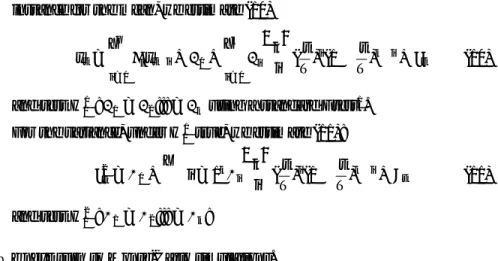
Table 1 returns the results of the simulations when one bases the test-ing strategy on the simple AICu criterion. The iid case is used to study the empirical size of the procedure, which is computed as 1 P (k = 0) or P (k = 1) [ P (k > 1). The four other cases are used to compute the empirical

Table 1: AICu based criterion for …ve models, the last four ones exhibiting ruptures in mean

iid case: H0 true

T = 50 T = 100 T = 150 T = 200 T = 500 P (k = 0) 0.813 0.831 0.860 0.872 0.882 P (k = 1) 0.102 0.090 0.088 0.066 0.075 P (k > 1) 0.085 0.079 0.052 0.062 0.043

Single discrete break in mean: H0 false

T = 50 T = 100 T = 150 T = 200 T = 500 P (k = 0) 0.125 0.018 0.006 0.001 0.000 P (k = 1) 0.400 0.329 0.187 0.109 0.006 P (k > 1) 0.475 0.653 0.807 0.890 0.994

Linear trend in mean: H0 false

T = 50 T = 100 T = 150 T = 200 T = 500 P (k = 0) 0.047 0.000 0.000 0.000 0.000 P (k = 1) 0.729 0.849 0.841 0.865 0.878 P (k > 1) 0.224 0.160 0.159 0.135 0.122

Stochastic trend in mean: H0false

T = 50 T = 100 T = 150 T = 200 T = 500 P (k = 0) 0.229 0.244 0.252 0.233 0.228 P (k = 1) 0.161 0.182 0.182 0.167 0.158 P (k > 1) 0.610 0.574 0.566 0.600 0.614

Stop-break mode: H0 false

T = 50 T = 100 T = 150 T = 200 T = 500 P (k = 0) 0.156 0.059 0.049 0.064 0.000 P (k = 1) 0.202 0.077 0.055 0.078 0.000 P (k > 1) 0.642 0.864 0.896 0.858 1.000

Note 1: The iid case returns the size of the procedure, given by 1 P (k = 0). Ideally it should be close to 0

Note 2: The other four cases return the power of the procedure, given by P (k = 1) [ P (k > 1). Ideally it should be close to 1

power, i.e. P (k = 1)[P (k > 1). Using the AICu criterion returns a low empiri-cal size, especially for small sample size (T = 50), not exceeding 0:187. Focusing on the power, results are twofold. For the stop-break model (Engle and Smith [1999]), the linear trend in mean, and the single discrete break in mean models,

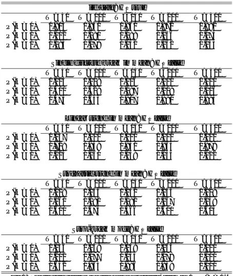
Table 2: Size and power of restriction tests at 4 nominal sizes for …ve models, the last four ones exhibiting ruptures in mean.

iid case: H0 true

size T = 50 T = 100 T = 150 T = 200 T = 500 0.01 0.045 0.039 0.024 0.020 0.011 0.05 0.105 0.086 0.063 0.051 0.045 0.10 0.139 0.120 0.093 0.088 0.070 0.15 0.166 0.148 0.111 0.105 0.092

Single discrete break in mean: H0 false

size T = 50 T = 100 T = 150 T = 200 T = 500 0.01 0.343 0.716 0.910 0.944 1.000 0.05 0.671 0.925 0.970 0.982 1.000 0.10 0.810 0.967 0.989 0.996 1.000 0.15 0.848 0.978 0.992 0.998 1.000

Linear trend in mean: H0 false

size T = 50 T = 100 T = 150 T = 200 T = 500 0.01 0.489 0.918 0.995 1.000 1.000 0.05 0.788 0.986 1.000 1.000 1.000 0.10 0.897 0.994 1.000 1.000 1.000 0.15 0.938 0.998 1.000 1.000 1.000

Stochastic trend in mean: H0false

size T = 50 T = 100 T = 150 T = 200 T = 500 0.01 0.512 0.467 0.442 0.442 0.432 0.05 0.689 0.652 0.639 0.638 0.654 0.10 0.739 0.718 0.695 0.717 0.729 0.15 0.763 0.741 0.736 0.751 0.749

Stop-break model: H0false

size T = 50 T = 100 T = 150 T = 200 T = 500 0.01 0.670 0.871 0.880 0.860 0.999 0.05 0.792 0.913 0.936 0.914 1.000 0.10 0.817 0.933 0.946 0.925 1.000 0.15 0.831 0.936 0.947 0.932 1.000

Note 1: The iid case returns the size of the procedure. Ideally it should be close to the nominal one

Note 2: The four other cases return the power of the procedure. Ideally it should be close to 1

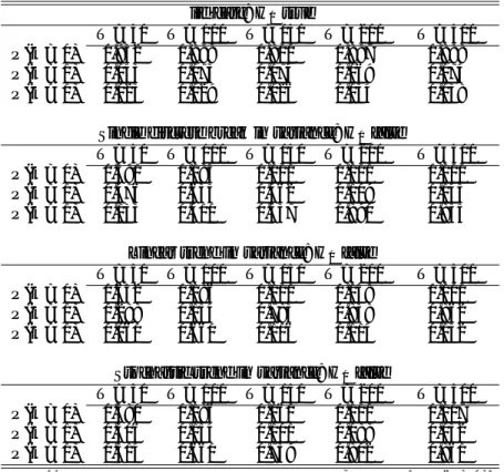
Table 3: AICu based criterion for four models, the last three ones exhibiting ruptures in variance

iid case: H0 true

T = 50 T = 100 T = 150 T = 200 T = 500 P (k = 0) 0.932 0.898 0.900 0.897 0.888 P (k = 1) 0.043 0.073 0.074 0.069 0.074 P (k > 1) 0.023 0.029 0.026 0.034 0.038

Single discrete break in variance: H0 false

T = 50 T = 100 T = 150 T = 200 T = 500 P (k = 0) 0.391 0.085 0.001 0.001 0.000 P (k = 1) 0.476 0.635 0.462 0.109 0.145 P (k > 1) 0.133 0.410 0.537 0.890 0.855

Linear trend in variance: H0false

T = 50 T = 100 T = 150 T = 200 T = 500 P (k = 0) 0.652 0.186 0.111 0.048 0.000 P (k = 1) 0.288 0.154 0.783 0.838 0.862 P (k > 1) 0.060 0.660 0.106 0.114 0.132

Stochastic trend in variance: H0 false

T = 50 T = 100 T = 150 T = 200 T = 500 P (k = 0) 0.380 0.186 0.160 0.110 0.107 P (k = 1) 0.306 0.154 0.101 0.088 0.032 P (k > 1) 0.314 0.660 0.739 0.802 0.861

Note 1: The iid case returns the size of the procedure, given by 1 P (k = 0). Ideally it should be close to 0

Note 2: The three other cases return the power of the procedure, given by P (k = 1) [ P (k > 1). Ideally it should be close to 1

the power ranges from 0:844 to 0:953 for T = 50. For the stochastic trend in mean model, the power is lower: ranging form 0:771 to 0:748 according to the sample size. Hence, results remain within an acceptable range.

Focusing now on restriction tests, as presented in Table 2, at the 5% nominal size, the empirical sizes range from 0:105 (T = 50) to 0:045 (T = 500). Also, as mentioned above, for the stop-break, the linear trend in mean, and the single discrete break in mean models, the type II error is close to the nominal size, except for T = 50. When the data contain a stochastic trend, the power ranges

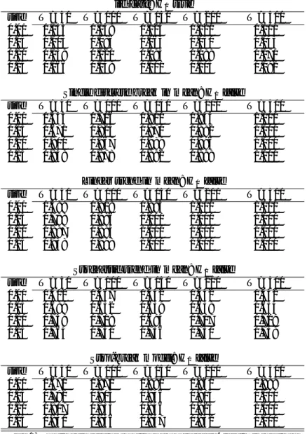
Table 4: Size and power of restriction tests at 4 nominal sizes for four models, the last three ones exhibiting ruptures in mean

iid case: H0 true

size T = 50 T = 100 T = 150 T = 200 T = 500 0.01 0.007 0.007 0.013 0.009 0.012 0.05 0.024 0.026 0.030 0.031 0.038 0.10 0.043 0.052 0.055 0.060 0.061 0.15 0.054 0.070 0.076 0.080 0.082

Single discrete break in variance: H0 false

size T = 50 T = 100 T = 150 T = 200 T = 500 0.01 0.109 0.459 0.768 0.913 1.000 0.05 0.305 0.729 0.947 0.985 1.000 0.10 0.447 0.839 0.980 0.995 1.000 0.15 0.538 0.880 0.988 0.998 1.000

Linear trend in variance: H0false

size T = 50 T = 100 T = 150 T = 200 T = 500 0.01 0.048 0.194 0.399 0.534 0.994 0.05 0.148 0.415 0.659 0.807 1.000 0.10 0.212 0.536 0.786 0.887 1.000 0.15 0.281 0.608 0.835 0.917 1.000

Stochastic trend in variance: H0 false

size T = 50 T = 100 T = 150 T = 200 T = 500 0.01 0.226 0.577 0.666 0.761 0.849 0.05 0.407 0.707 0.765 0.825 0.864 0.10 0.502 0.776 0.795 0.853 0.873 0.15 0.577 0.792 0.818 0.871 0.882

Note 1: The iid case returns the size of the procedure. Ideally it should be close to the nominal one

Note 2: The three other cases return the power of the procedure. Ideally it should be close to 1

form 0:639 to 0:689, at 5% suggesting using a higher threshold in empirical work. Turning now to structural breaks in variances, four cases are considered:

f (t) = 1 and thus ct= "t; "t N (0; 1) (iid case),

f (t) = 1 for t t0 and

p

f (t) = 2 otherwise, "t N (0; 1); and t0 is

f (t) = (1 + 2t=T ); "t N (0; 1) (variance trend),

f (t) = exp(ht=2), ht = ht 1+ t, t N (0; 1); "t N (0; 1) (stochastic

volatility model)

Table 3 presents the size and power of the procedure based on the AICu decision rule. Clearly, the size is low, but unexpectedly doesn’t decrease with the sample size. Considering the power, it is quite low for T = 50; especially when the variance moves according to a linear trend and generally for all considered models. It is nevertheless acceptable for sample sizes ranging from T = 100 to T = 500. Turning now to restriction tests, Table 4, it can be seen that the empirical size is less than the 5% nominal one. Focusing at last on the type II error; it appears that the test has power against the three models, only for sample sizes more or less than T = 100 (T = 150 for linear trend in variance). In all cases under the alternative, the test has low power for small sample sizes (T = 50).

4

Conclusion

In this note, we have introduced a procedure to test for the null of no struc-tural change in the …rst two moments of a conditional distribution of a time series. The procedure uses Bernstein polynomials to extract the (noisy) signal and has not the nuisance parameter problem under the alternative. Two tests are proposed, a test based on the simple AICu criterion, and a restriction one. Monte-Carlo simulations suggest that the test is powerful and can be used in empirical work. Moreover, the procedure could be used as a general misspeci…-cation test.

References

[1] Andrews, W.K., Lee, I. & W. Ploberger (1996), Optimal Change Point Tests for Normal Linear Regression, Journal of Econometrics 70, p. 9-38.

[2] Bai, J. & P. Perron (1998), Estimating and testing linear models with multiple strucural changes, Econometrica 66, p.47-78.

[3] Charfeddine, L. & D. Guégan (2011), Which is the best model for the US in‡ation rate : A structural changes model or a long memory process ? to appear in Journal of Applied Econometrics.

[4] Diebold, F.X. & A. Inoue (2001), Long memory and regime switching, Journal of Econometrics 105, p. 131-159.

[5] Engle, R.F. & A.D. Smith (1999), Stochastic permanent breaks, The Review of Economics and Statistics 81, p.553-574.

[6] Granger, C,. & C. Starica (2005), Nonstationarities in Stock Returns, The Review of Economics and Statistics 87, p. 503-522.

[7] Guégan, D. (2010), Non-stationary samples and meta-distribution. In: Basu A, Samanta T, SenGupta A, (eds.) ISI Platinium Jubilee Volume: Statistical sciences and interdisciplinary research, ICSPRAR World Scien-ti…c Review, in press.

[8] Heracleous, M.S., Koutris, A. & A. Spanos (2008), Testing for nonsta-tionarity using maximum entropy resampling: A misspeci…cation testing perspective, Econometric Reviews 27, p. 363-384.

[9] McQuarrie, A.D.R. & C.-L. Tsai (1998), Regression and time series model selection, World Scienti…c.

[10] Perron, P. (1989), The Great Crash, the oil price shock and the unit root hypothesis. Econometrica 57, p. 1361-1401.

[11] Perron, P. (2005), Dealing with Structural Breaks, in Palgrave Handbook of Econometrics, Vol. 1: Econometric Theory.