HAL Id: halshs-00344845
https://halshs.archives-ouvertes.fr/halshs-00344845
Submitted on 5 Dec 2008
HAL is a multi-disciplinary open access
archive for the deposit and dissemination of
sci-entific research documents, whether they are
pub-lished or not. The documents may come from
teaching and research institutions in France or
abroad, or from public or private research centers.
L’archive ouverte pluridisciplinaire HAL, est
destinée au dépôt et à la diffusion de documents
scientifiques de niveau recherche, publiés ou non,
émanant des établissements d’enseignement et de
recherche français ou étrangers, des laboratoires
publics ou privés.
The pollution haven hypothesis : a geographic economy
model in a comparative study
Sonia Ben Kheder, Natalia Zugravu
To cite this version:
Sonia Ben Kheder, Natalia Zugravu. The pollution haven hypothesis : a geographic economy model
in a comparative study. 2008. �halshs-00344845�
Documents de Travail du
Centre d’Economie de la Sorbonne
Maison des Sciences Économiques, 106-112 boulevard de L'Hôpital, 75647 Paris Cedex 13
http://ces.univ-paris1.fr/cesdp/CES-docs.htm
The pollution haven hypothesis : a geographic economy
model in a comparative study
Sonia B
ENK
HEDER,Natalia Z
UGRAVUThe pollution haven hypothesis: a geographic economy model in a
comparative study
BEN KHEDER Sonia
yZUGRAVU Natalia
zApril 2008
Abstract
Although based on theoretical foundations, the pollution haven hypothesis has never been clearly proven empirically. In this study, we reexamine this hypothesis by a fresh take on both its theoretical and empirical aspects. While applying a geographic economy model on French …rm-level data, we con…rm the hypothesis for the global sample. Through sensitivity analysis, we validate it for Central and Eastern European countries, emerging and high-income OECD countries, but not for the major part of the Commonwealth of Independent States countries. Finally, we show that the pollution haven hypothesis is con…rmed in the strongest manner for emerging economies.
Keywords: FDI; Environmental regulation; Economic geography; Pollution haven hypothesis. JEL classi…cation: F12; F18; Q28
1
Introduction
There is, by now, quite an extensive literature on the factors that in‡uence …rms’location decisions abroad. Among these factors, the most studied are the cost of production factors such as labor and capital, and the mar-ket access. Additional factors such as taxation or agglomeration e¤ects have also been studied. More recently, a new factor appeared as a potential determinant of …rms’location abroad: environmental regulation. This factor was notably put in evidence by Copeland and Taylor (2004) through a simple model of specialization and trade according to which the rich countries, that protect their environment, should abandon their polluting activities to developing countries, whose environmental legislation and enforcement are not severe. This statement illus-trates the commonly studied "pollution haven hypothesis" (PHH). Nevertheless, empirical research often fails
We thank the Directorate of Treasury and Economic Policy (DGTPE in French) for having allowed us to exploit data from the Subsidiaries-Survey 2002. We also would like to thank Ann E. Harrison, Katrin Millock, Edward Norton, and the participants of the Development and Transition ROSES and CERDI joint seminar, and the Environmental Economics seminar of Centre d’Economie de la Sorbonne for their helpful comments on previous versions of this article. Natalia Zugravu thanks in particular the ADEME (The French Environment and Energy Management Agency) for the …nancial support granted for the completion of her Ph.D. dissertation. Any errors or shortcomings remain the authors’ own responsibility.
yCES - Université Paris-I Panthéon Sorbonne, 106-112 boulevard de l’Hôpital, 75013 Paris, FRANCE (e-mail:
zCorresponding Author. CES - Université Paris-I Panthéon Sorbonne, Maison des Sciences Economiques, 106 -112 boulevard de
l’Hôpital, 75647 Paris Cedex 13, FRANCE. E-mail: [email protected], Bureau 227, Tel : + 33 1 44 07 82 66, Fax : +33 1 44 07 81 91.
to prove this hypothesis. Furthermore, an approach based on the classic theory of endowments would yield an opposite conclusion: polluting activities are generally capital-intensive and should thus locate in rich countries where capital is abundant.
The debate on the pollution haven hypothesis produced a political challenge by trying to …nd clear empirical evidence in order to prove or refute what is really a complex and dynamic issue: how does environmental regulation interact with more and more mobile production?
Generally, statistical studies prove that the pollution haven hypothesis cannot be clearly identi…ed. Four potential problems in this literature require more empirical tests. First of all, most studies lack theoretical foundations for the construction of the equations to be tested, which often entails speci…cation errors. Secondly, the studies of Zhang and Markusen (1999) and Cheng and Kwan (2000) demonstrate the importance of relative endowments of production factors in the explanation of the foreign direct investment (FDI). The absence of this determinant can lead to omitted variable bias. Next, Levinson and Taylor (2008) and Keller and Levinson (2002) emphasize the empirical importance of controlling for the unobservable characteristics of industries and locations. Finally, as noted by Smarzynska and Wei (2004), several studies use very aggregated data on FDI, and proxies of the severity of the environmental policy that are far o¤ the real variable to be taken into account, which generally results in bias induced from measurement-error.
In this study we considered these various limits and tried to remedy them by di¤erent means. Consequently, we present a classic theoretical model of geographic economy (open economy model with increasing returns to scale, monopolistic competition and trade costs), which supplies us a testable equation for determinants of the …rms’location choice, among which we distinguish the impact of the environmental regulation. According to our knowledge, at the moment, there is no empirical study on the link between FDI and environment, in particular on the pollution haven hypothesis, based on a theoretical model of geographic economy. Such models are used in some purely theoretical studies, without empirical estimation of the forces at work (e.g., Rauscher, 2005; Conrad, 2005; Van Marrewijk, 2005). The geographic economy model presents the advantage to take into account the complexity of FDI determinants, such as: production factor endowments (labor, capital, etc.); distance between trade partners, local market size and access to other important markets (market potential of the host country); cultural, historic, linguistic connections. While representing the demand, the market potential derived from theory has the advantage, in comparison to other often used variables (GDP, population, etc.), to take into account the accessibility to the host country’s market and that of its neighbors, the trade barriers and competition. Besides, the additional interest of this model is that it enables us to introduce the environmental regulation as a determinant of the location decision. Thus, for the speci…cation of the location choice, we are inspired by the study of Head and Mayer (2004), to which we introduce environmental regulation. Besides labor and capital, we consider pollution as a production factor, the cost of which is the pollution tax established exogenously by the government. Furthermore, in our empirical model, the …xed costs corresponding to the launch of an activity / creation of a …rm di¤er across countries and thus have an impact on the …rm’s location choice. These costs are proxied in our study by the institutional quality of the potential locations.
countries, while also considering other groups of countries. In fact, if in 1992 the transition and developing countries counted 30 % of the French multinationals’subsidiaries, in 2002 these countries were the destination of 45% of the French …rms abroad. Concerning the speci…c case of the Central and Eastern European Countries (CEECs) and the countries of the Commonwealth of Independent States (CIS), between 1992 and 2002 the French multinationals multiplied by six the number of their subsidiaries in this region in order to represent 11% of the total of the French …rms abroad (3 % in 1992)1. Regarding emerging countries, while they counted about
25% of the French establishments in 1992, in 2002 they counted about 35%. This important reorientation of the French FDI towards countries with an environmental regulation less severe than that of industrial nations represents an interesting case study for the research on the pollution haven hypothesis.
Furthermore, to represent the environmental regulation’s stringency in a more complete way, we create a complex and dynamic index which estimates the relative severity of the environmental policy between countries, based on a diverse set of variables.
Finally, in order to take into account the speci…c characteristics of industries and countries, the empirical estimations are performed by controlling for di¤erent types of industrial sectors (according to their pollution intensity) and groups of countries (transition CEECs, transition countries of CIS, emerging countries2, and
high-income OECD countries3).
The contribution of this article lies in the empirical estimation and test of the pollution haven hypothesis, using …rm level data on worldwide location of French manufacturing subsidiaries. Our empirical results show that looking at diverse countries (pooled sample), the French …rms of the manufacturing sector, and in particular the ones belonging to more polluting sectors, prefer to settle in countries where the environmental regulation is the most lenient, thereby con…rming the pollution haven hypothesis. Sensitivity analysis including interaction terms between the environmental regulation and the di¤erent country groups generate three major conclusions. First of all, we validate this hypothesis for all the CEECs, emerging and high-income OECD countries in our sample. Concerning the CIS transition countries, we discover a prevailing opposite relationship: it is rather the lenient environmental regulation that deters the foreign investments. Finally, we show that emerging economies constitute the group of countries for which this hypothesis is most clearly con…rmed.
This study is structured as follows: in section 2 we present the relevant literature analyzing the relation between FDI and environmental regulation. In the third section, we describe brie‡y the theoretical model of the new geographic economy giving the econometric speci…cation for the analysis of the determinants of …rms’ location decision. The fourth section describes the empirical model and data used. In the …fth section we analyze the empirical results and provide some extended analyses. The last section concludes.
1Source : Survey on French subsidiaries implanted abroad, managed by the Directorate of Treasury and Economic Policy on
2003.
2An emerging country is a country, up to there under developed, which undertaken measures and accumulated means, in
particular legal and cultural, in order to begin a phase of fast growth of the production and social welfare. According to Morgan Stanley Emerging Markets Index, in July 2006, the status of emerging country was awarded to the following countries: Argentina, Brazil, Chile, China, Colombia, Egypt, Iran, India, Indonesia, Israel, South Korea, Malaysia, Mexico, Morocco, Pakistan, Peru, the Philippines, South Africa, Sri Lanka, Taiwan, Thailand, Tunisia, Turkey, Venezuela.
3High-income OECD members except Czech Republic and Republic of Korea, considered here as transition and emerging
2
Review of the literature
The increasing relocation of industries towards developing countries raises some questions, mainly in the …eld of employment, and more recently concerning the environment. The relatively less severe environmental regulation in developing countries can create a comparative advantage in pollution-intensive production, and trade openness and FDI could then damage the environment of the host country. From a theoretical point of view, researchers proposed two main hypotheses to explain the direct impact of international trade and FDI on the environment: the "pollution haven hypothesis" and the "factor endowment hypothesis". The …rst hypothesis assumes that countries are identical except for exogenous di¤erences in their environmental policies. Thus it is cheaper to produce pollution-intensive goods in countries with a weaker environmental regulation, usually poorer countries. Trade, inferred by di¤erences in environmental policy, thus creates pollution havens in the poorer countries. The "factor endowment hypothesis" is the main alternative to the pollution haven hypothesis. It suggests that trade is determined by the relative abundance of production factors (labor and capital in most models) in each country. Thus, if pollution-intensive goods are generally more capital intensive, they should be produced in the developed countries, instead of the developing countries. At the same time, the developed countries are supposed to be abundant in capital and have a stricter environmental policy, unlike poor countries. This illustrates the narrow connection between both hypotheses, which should be taken into account while testing anyone of them.
Unfortunately, the empirical validation of the pollution haven hypothesis is always rather delicate. One of the founder-articles is Grossman and Krueger (1993), which however shows that the trade liberalization between the United States and Mexico in the 1980’s and 1990’s did not come along with a relocation of polluting industries, which could be explained by the very weak weight of environmental costs imposed on American …rms during this period. Since then, articles on this subject followed without a consensus being established, while concerns abound about the e¤ects of environmental standards on trade ‡ows and FDI. However, the scienti…c research did not manage to prove that environmental regulation a¤ects trade or …rms’investment decisions (e.g., Ja¤e et al., 1995; Wheeler, 2001).
Ederington et al. (2005) explain partially why previous studies did not con…rm the pollution haven hypoth-esis. They recall that international trade is essentially made between developed countries, whose regulation is quite similar. However, if one examines only the ‡ows between industrial nations and developing countries, the environmental standards have more pronounced e¤ects on the trade structure: with the strengthening of the environmental regulation of the United States, imports from developing countries decrease. In fact, Ederington et al. (2005) notice that polluting industries are generally the least mobile geographically and thus, it becomes more expensive to establish production in countries that apply a less rigorous regulation.
Most studies in this …eld use data on trade ‡ows while analyzing the pollution haven hypothesis. Some more recent papers examine this hypothesis by using data on FDI. Eskeland and Harrison (2003) study the e¤ect of the abatement cost and pollution intensity on FDI in Morocco, Cote d’Ivoire, Venezuela and Mexico, and …nd essentially no empirical support for the pollution haven hypothesis. Besides, they …nd that the United States
factories are appreciably more e¢ cient in terms of energy use and employ more "clean" types of energy than the host country’s plants. In a group of 24 transition countries, Smarzynska and Wei (2004) …nd some, however relatively weak, proof for the pollution haven hypothesis.
Dean et al. (2004), in a study on China, discover a relationship between FDI and environmental regulation completely di¤erent from that evoked by the pollution haven hypothesis. In fact, the authors …nd that a less stringent regulation is a signi…cant determinant for Chinese villages’attractiveness for joint ventures with partners from Hong-Kong, Macao, Taiwan and other countries of South Asia. On the contrary, industrial nations (United States, Japan, United Kingdom etc.) are attracted by higher standards, regardless of industry pollution intensity. The authors suggest that this result could be explained by technological di¤erences.
Other studies, however, assert that environmental regulation in‡uences the spatial allocation of capital. A seminal paper in this literature is that of Keller and Levinson (2002). What distinguished this work was its using of, on the one hand, panel data on inward FDI ‡ows in the United States over a long period of time and, on the other hand, an innovative measure of the relative abatement costs across the States. By applying standard parametric models on panel data, the authors …nd a robust result showing that abatement costs had moderate dissuasive e¤ects on foreign investments. Given the implications of such a conclusion for trade and environmental policies, any evaluation of the sensibility of these results to changes in the parametric hypotheses is well justi…ed. The application to Keller’s and Levinson (2002) data of the recently developed non parametric techniques (Henderson and Millimet, 2007) reveals two results: …rst, some of the parametric results are not robust, and second, the impact of relative abatement costs is not uniform across the States, and is generally of a smaller magnitude than previously suggested.
Finally, a recent study (Cole et al., 2006) shows the existence of an inverse relationship between FDI and environmental regulation: it is FDI that in‡uences the environmental policy, but this e¤ect is a function of the degree of corruption in the host country. The authors show that at high (low) corruption levels, FDI leads to less (more) stringent environmental policy.
Di¤erent theoretical and empirical factors can explain the lack of robust empirical proof for the pollution haven hypothesis. One reason for which developing countries do not tend to become pollution havens can be the fact that the stringency of the environmental standards is only one, and maybe not the most important, factor determining the comparative advantages between countries. In particular, the endowments of factors such as quali…ed human capital and physical capital determine largely industrial location and the products that a country will export. As far as the strongly polluting industries tend also to be intensive in capital, the relative lack of capital in the developing countries can prevail over the advantage of low abatement costs (e.g., Antweiler et al., 2001; Cole and Elliott, 2002).
It is thus di¢ cult to conclude on this point, in so far as the laxness of the environmental policy, supposed to attract polluting …rms, may be associated with other characteristics that, in their turn, generally discourage the establishment of foreign …rms. It is notably the case of weak institutions, expressed through high corruption level, lack of civil freedoms’and property rights’protection, etc. That is why, as Smarzynska and Wei (2004) underline, it is necessary to take into account the e¤ect of institutions on FDI, while trying to test the pollution
haven hypothesis.
3
Theoretical background
The theoretical frame of our model is based on the classic hypotheses of the new geographic economy, open economy model with increasing returns to scale, monopolistic competition and trade costs. Monopolistic competition is a common market form, characterized by the following: there are many producers and many consumers in a given market; consumers have clearly de…ned preferences and sellers attempt to di¤erentiate their products from those of their competitors; goods and services are heterogeneous, usually (though not always) intrinsically so; there are few barriers to entry and exit; producers have a degree of control over price. This frame seems relevant to our study since these criteria characterize well the French market.
Moreover, the existence of intra-industry trade is typically associated with increasing returns to scale, product di¤erentiation and monopolistic competition (Helpman and Krugman, 1985), and the volume of such trade is expected to be higher the greater the equality of trading partners’GDP per capita (Helpman, 1987). Hummels and Levinsohn (1995), however, in repeating Helpman’s (1987) analysis for a sample of non-OECD countries, found that gravity models still worked well for a group of countries whose bilateral trade was more likely characterized by homogeneous goods. Evenett and Keller (2002) have argued that the gravity model can nest both the increasing returns/product di¤erentiation story as well as a more conventional homogeneous goods/relative factor abundance story. Thus, we can use the monopolistic competition model in order to explain French multinationals’behavior concerning location in both the developed and developing countries.
In our model, the world consists of i = 1; :::N open economies. In every country there are two sectors - industry and agriculture. Given the interest of this paper in the industry’s location, we model the second sector as simply as possible. Namely, the traditional sector A is supposed to produce a homogeneous good under Walrasian conditions (constant returns to scale and perfect competition), which is traded costlessly. The manufacturing sector M produces a continuum of di¤erentiated goods, called varieties v, under increasing returns to scale in an environment of monopolistic competition à la Dixit and Stiglitz (1977). Each …rm produces a distinct variety. Let us denote the elasticity of substitution between two varieties > 1. The shipping of these varieties towards another country implies "iceberg" transport costs: > 1 units must be sent so that a unity arrives at the destination; the rest, 1, is melt in transit. The consumers spend a part 0 < < 1 of their income E on the purchase of the composite good M , the rest is spent on the good A, and they have constant elasticity of substitution (CES) sub-utility functions for the composite good. Under constraints of income and each variety’s price, the maximization of this sub-utility results in the following demand function of the country’s j consumers for a speci…c variety h produced in a country i (see details in Appendix A):
qij(h) = [pi(h) ij] P i R ni[pi(v) ij] 1 dv Ej (1)
country i, i 2 N; and ij is the trade cost supported by the consumer in the importing country j. The trade
cost includes all transaction costs connected to the shipment of goods in space and across borders.
One of the most important factors for the …rm’s location decision is the production cost. The total production cost in every potential location is supposed to take the following form: ciqi+ Fi. The increasing returns result
from …xed costs Fi(h) speci…c to the …rm producing a variety h (further named …rm h) and related to launching
activity in the country i, qi(h) is the total production of the …rm h in the country i and ci(h) is its constant
production marginal cost. A …rm tries to maximize its gross pro…t on every market. We can write the gross pro…t realized in any country j by a …rm h implanted in a country i:
ij(h) = [pi(h) ci(h)] ijqij(h) (2)
In this model à la Dixit and Stiglitz (1977) and Krugman (1980), the production price is a simple mark-up on the marginal cost: p = c( 1). By substituting it in the equation (1), we obtain the following expression for the quantity that a …rm h produces in country i and would ship to any destination j:
qij(h) = 1 [ci(h) ij] P i R ni[ci(v) ij] 1 dv Ej (3)
By replacing the expression (3) and the price expression in the equation (2), by summarizing the gross pro…ts realized by a …rm h located in country i while shipping its goods to any market j (equation 2) and by deducting the …rm’s …xed cost Fi(h), we obtain the total net pro…t that a …rm h could earn in any potential location i:
i(h) = ci(h)1 X j ij Ej Gj Fi(h) = ci(h)1 M Pi Fi(h) (4) with ij = 1ij , Gj = Pi R ni[ci(v) ij] 1 dv and M Pi = Pj ij Ej
Gj . The location choice is thus
deter-mined by the comparison of the characteristics of every potential location: demand (represented by M Pi, an
abbreviation of the Market Potential concept developed in section 4), cost of launching an activity/ creating an enterprise, and production cost.
Taking logarithms and denoting i=ci(h)
1
M Pi, we write the pro…tability U of a …rm h located in country
i:
Ui(h) ln i(h) = ln ( i Fi(h)) = ln i+ ln 1 e(ln Fi(h) ln i) (5)
We have thus:
Ui(h) ln M Pi ( 1) ln ci(h) ln + ln 1 e(ln Fi(h) ln i) (6)
In our model, there are three production factors: K - capital, L - labor and P oll - pollution (the last factor is used only in industry). One of the most common forms used to represent the cost function is that of Cobb-Douglas with constant returns: c = A1w r t , where = 1 ( + ) and w, r and t are costs of labor,
capital and pollution, respectively. The share of labor in the …rm’s production process is noted by , of the capital is and …nally that of the pollution is , whereas A represents the total factor productivity. With this last speci…cation we can rewrite equation (6) in the following way:
Ui(h) ln M Pi+ ( 1) ln Ai (h) ( 1) ln wi (h) ( 1) ln ri
(h) ( 1) ln ti ln + ln 1 e(ln Fi(h) ln i) (7)
The equation (7) predicts that the pro…tability of a …rm settled in a country is an increasing function with regard to the market potential and the global factor productivity in this country, and decreasing with regard to …xed and production costs. For more simplicity, we present this relation as follows:
Ui(h) f ln M P
+ ; ln A+ i; ln wi; ln ri; ln ti; ln Fi (8)
This speci…cation represents the theoretical background for the empirical work that now follows.
4
Empirical work
4.1
A location choice model: the conditional logit
In this paper, we seek to study the factors determining a speci…c …rm single choice between some unordered alternatives. Each subsidiary h chooses country i where it will locate. An unordered choice model particularly well adapted to our question is the model developed by McFadden in 1974, i.e., the conditional logit (…rm …xed-e¤ects logit model).
The conditional logit is a discrete choice model based on pro…t maximization. In such a model, each …rm compares the pro…ts related to the di¤erent location alternatives, and selects, among the N alternatives, the location that will maximize its pro…t i(h):
In our example, for a French …rm h facing N alternatives, the pro…tability of choosing i can be written
i(h) = 0Zi+ "hi (9)
with Zia vector of independent variables that vary between location alternatives, the vector of estimated
parameters and "hi a random error term, which corresponds to unobserved variables related to location i and
a¤ecting the choice of …rm h.
Each French subsidiary h, faced with N choices, will select a location i if the expected pro…t i(h) exceeds
the expected pro…ts j(h), for all j 2 N alternative locations.
The model is made operational by a particular choice of distribution for the disturbances. Let Yh be a
random variable that indicates the choice made. Following McFadden, if and only if the N disturbances are independent and identically distributed with Weibull distribution, the probability that …rm h chooses location
i is given by: P r(Yh= i) = exp( 0Zi)= N P j=1 exp( 0Zj) (10)
This intuitive formulation of the conditional logit model presents nevertheless some limits due to the as-sumption concerning the disturbances, which implies the property of Independence from Irrelevant Alternatives (IIA). According to the IIA property, the likelihood of making a choice is independent of the other alternatives. In practice, this assumption could be problematic. In order to mitigate this problem, in our econometric speci-…cation we introduce in addition to the explanatory variables, dummy variables representing the four di¤erent country groups forming our sample. With the assumption that the error terms are correlated only within coun-try groups and not across groups, the dummy variables (de…ned in section 5) should capture this correlation and reduce the IIA problem.
4.2
Data description
Dependent variable
The location choice
Data concerning French …rms location choice have been gathered from the Survey about French …rms located abroad, conducted by the Directorate of Treasury and Economic Policy (DGTPE in French) in 2002. This Department collects from French Economic Missions abroad the census of units whose capital is owned by a French parent company by at least 10%. The survey includes among other information, the units date of creation and their French classi…cation NAF93 code, data which is crucial for this analysis. The global database covers 21379 investment decisions realized in all economic sectors in 128 countries during the past century. In our study, we concentrate on the manufacturing industry, excluding the two-level NAF93 code DF "Coke, Petroleum Re…ning and Nuclear Industry" which corresponds to speci…c sectors whose location determinants are beyond the scope of this study. In the end, reduced to manufacturing sectors and limited to data availability for the explanatory variables, our empirical sample covers 1332 French investments in 55 countries from 1996 to 20024.
Explanatory variables
As we have seen in our theoretical model, the pro…tability of a location for a …rm depends on the market potential of the location and its total factor productivity, the …rm’s production costs, and the …xed costs that correspond to launching an activity. We have calculated market potential and total factor productivity growth, following commonly used methods described hereafter. Production and …xed costs are represented using several proxies that we present below.
The market potential
The market potential is a general concept regarding the impact of demand on …rms location. Gross domestic product of the host country or its population are the most commonly used proxies for demand variables, but they
are very partial. Indeed, measuring the local demand through these variables present the major inconvenience to not take into account the demands emanating from nearby countries and the facility or di¢ culty to reach them. In this study we exceed these limits by using the concept of market potential of a location. Here, market potential (M P ) means "demand accessibility". This concept was introduced by Harris (1954) who proposed, as measure of the potential demand that a …rm faces, the sum of economic sizes of surrounding markets weighted over distances: M Pi=PNj=1GDPdistijj: The concept was then validated by its deduction from the standard model
of the new trade theory, such as presented in the equation (4) (Krugman, 1992; Head and Mayer, 2004). The presentation of the market potential à la Harris is very insu¢ cient because of omission of the price index, Gj, which allows taking into account the e¤ect of the competition. Besides, this simpli…cation supposes that
the simple distance includes all costs, while the literature on the border e¤ects on trade between countries refutes this hypothesis by underlining the importance of obstacles bound to borders (McCallum, 1995; Head and Mayer, 2000). In this study analyzing the determinants of French …rms location choice, it seems then essential to consider, besides the distance, additional trade costs induced by crossing borders and sharing or not a common language, while estimating the market potential of all possible destinations. Following Redding and Venables (2004) and Head and Mayer (2004), we build a measure of market potential that aggregates the local demand and the demands emanating from nearby markets, while taking into account the e¤ect of demand’s depreciation due to obstacles related to shipping goods in space and across borders. The estimation technique is presented in Appendix B.
Moreover, given that market potential values have been calculated using estimators of trade regression5, the standard-errors of equation (10) are biased as they include also trade equation’s errors. We use the bootstrap technique in order to obtain correct standard-errors (limiting also measurement-error-induced bias resulting from using a calculation technique for total factor productivity variable). Standard-errors reported in clogit regressions table are thus based on 100 bootstrap replications (see Efron and Tibshirani, 1993, for more details).
Total factor productivity
While there is no available data on total factor productivity , we apply here a "Growth Accounting" calcu-lation method, following the technique developed by Robert Solow (1956) to calculate the rate of technological progress (T F P _growth). According to this technique, the sources of output growth are: contribution of capital growth = KK; contribution of labor growth = LL; and contribution of total factor productivity growth =
T F P
T F P . To resume, the technological progress in our study equals output growth which is not explained by
factors growth (T F P _growth = P IB P IB K K L L ) 6. Factor costs
Following our theoretical model, the total production cost faced by a …rm is composed by labor, capital and environmental costs.
Suitable variables to re‡ect the capital and the labor costs would have been respectively the capital interest rate and the wages in manufacturing sectors. On account of many missing values in the International Labor
5Cf Appendix B.
6The coe¢ cients and are obtained by running regression: ln P IB = ln K + ln L + ", for each of our country-groups,
O¢ ce Laborsta database, related to international labor costs, and because of an expected high correlation between these costs and governance factors, we have …nally decided to capture capital and labor costs through the countries’relative endowments in production factors. This is represented by the variable KL, which is the ratio K/L, with K the capital stock7 and L the total labor force.
The most complex cost to be represented is the environmental regulation (ER). Since a direct measure does not exist for this cost, we had recourse to di¤erent proxies that allowed us to compute, through the Z-score method8, a global and quite exhaustive Environmental Regulation index (ER index) for each country in our
sample. This index integrates the following variables:
Multilateral Environmental Agreements (MEA rati…ed): this variable distinguishes countries having rati…ed several international environmental agreements. Thus, countries ratifying more MEAs prove their governments’ concern about environmental protection. We retained the MEA’s rati…cation year (and not the year of signature) since it is the rati…cation that imposes compliance to international environmental treaties.
ISO 14001 (ISO 14001 certi…cations/billion US$ GDP): we have integrated for each country the number of ISO 14001 certi…cations normalized by the country’s GDP. Even if ISO certi…cation is a private and voluntary initiative, this variable manages to express a global state of mind prevailing in a country. For illustration, this variable is also used in the construction of the Environment Sustainability Index jointly initiated by the Yale Center for Environmental Law and Policy and Columbia University. On one hand, one can suppose that a higher number of 14001 ISO certi…ed …rms is the consequence of strict standards and controls imposed by the government. On the other hand, countries where this variable is the most important should be considered as countries where population is the most sensitive to environmental issues and thus the most exacting to environmental policy’s severity.
International NGOs (INGOs’ members/million of population): this variable represents the density of in-ternational non-governmental organizations with membership. As mentioned by Dasgupta et al. (1995) and Smarzynska and Wei (2004), international NGOs make local population sensitive to environmental problems, and also put pressure on governments to respect laws. Thus, a more important presence of international NGOs in a country would imply a more stringent environmental regulation.
Energy e¢ ciency (GDP/unit of energy used): the interest of using such a quantitative variable is that it gives a real measure of the impact of the preceding variables9. This allows distinguishing countries that apply concrete environmental measures from the ones that adopt a "theoretical" environmental policy not really restrictive to …rms.
Thus, grouping these variables in a single index allows us to encompass the general environmental regulation
7The capital stock is calculated by using the following formula: K
t= gross …xed capital formationt + 0.95 capital stockt 1.
Due to data availability (particularly concerning transition countries), the initial stock is represented by the gross …xed capital formation in 1990.
8We …rst calculate for each variable and year, the distance between each country’s value and the mean of the group expressed
in standard-errors, following the formula: z = Xjt Xt = t. We obtain thus values allowing to classify the countries below
or above the mean. Then, we calculate the unweighted average of all variables’ z-scores. Finally, we apply the standard normal percentile technique which gives the value 0 to the least average Z-score and 100 to the highest. Thus, the value 50 corresponds to the mean of the sample.
9A more appropriate quantitative measure would have been the manufacturing sectors’CO
2 emissions normalized by the value
added in the respective sectors. Due to a lack of consistent data that would have prevented us from including several countries, we have preferred to consider energy e¢ ciency, which generates similar results (available upon request).
of countries according to di¤erent more precise environmental aspects. For instance, some countries can have a small number of ISO 14001 certi…ed …rms, but high energy e¢ ciency. The use of one variable rather than the other in the regression would then give an incomplete vision of the local environmental regulation and result in wrong ER coe¢ cients. As illustration, we can cite the work of Smarzynska and Wei (2004) who, by using several too precise environmental variables, taken separately in the estimations, did not manage to capture the general aspect of the environmental regulation, which may have prevented them from proving explicitly the pollution haven hypothesis. Moreover, introducing a unique proxy for environmental regulation stringency can lead to biased results. For example, if we only use the MEA variable as the environmental proxy without controlling for other aspects of the environmental policy climate, it could capture in this case the state’s willingness to keep reliable relationships on international arena, which is usually favorable for FDI, rather than its direct concern to international, and much less domestic environmental compliance.
Table 1 presents correlations among the four variables and the ER index. On the one hand, some variables are well correlated, e.g., ISO 14001 and NGO variables (0.46), or MEA and Energy e¢ ciency variables (0.39), while others, e.g. ISO 14001 and Energy e¢ ciency, have a correlation coe¢ cient close to zero (0.092). On the other hand, we can see in the …rst column that all variables are strongly enough positively correlated with the ER index. This lends support to our argument that these variables measure each one a di¤erent aspect of environmental stringency, and that taken together they represent environmental stringency in general.
Table 1 here
-Governance factors
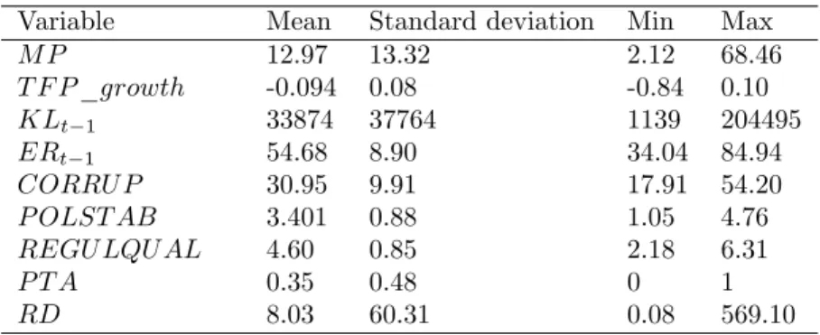
Since there is no variable representing precisely a …rm’s …xed costs to establish itself in a location, we have used proxies of institutional quality in a location in order to capture these costs. Indeed, bad governance generates additional costs while launching an activity and creates a feeling of insecurity among investors. Factors related to country governance constitute then determining factors to …rms’location abroad, especially when we consider developing countries or transition economies, where governance problems are rather frequent. In our paper, we use as proxies three governance indicators developed by Kaufmann et al. (2005): the corruption level (CORRU P ), the political stability (P OLST AB) and the government regulatory quality (REGU LQU AL). CORRU P is the inverse of the original Kaufmann index which re‡ects the control of corruption in states ( a higher value meaning a better governance outcome). Our corruption variable should then have a negative e¤ect on location decisions as a result of greater corruption. At the opposite, we expect the attractiveness of a location to increase with political stability and absence of violence (P OLST AB), and the government ability to implement promoting regulations (REGU LQU AL). Tables 4 and 5 in Appendix present descriptive statistics for the independent variables and information about the data.
5
Empirical results
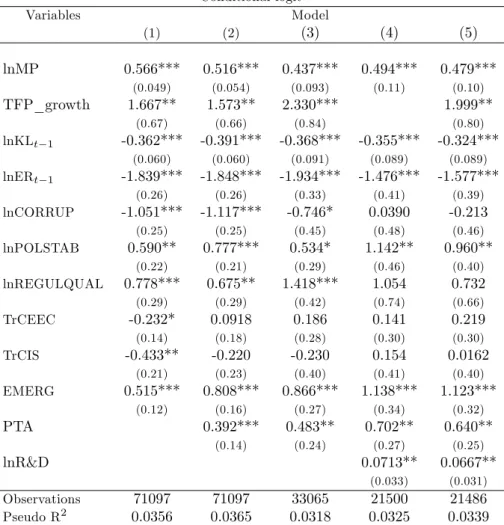
Table 2 shows estimation coe¢ cients concerning the impact of di¤erent factors on the location of French …rms. Besides variables presented in the preceding section, our estimations include also dummy variables that we have created by grouping countries in four homogenous clusters: T rCEEC for transition CEECs, T rCIS for transition countries of CIS, EM ERG for emerging countries, and OECD for high-income OECD members. Variables are log-linearized, and KL and ER have been lagged one-year to avoid any possible endogeneity with the dependent variable.
Our base model, estimation (1), shows results consistent with theory and our predictions for all the explana-tory variables. First, concerning our core variable in this study, environmental regulation, it seems to be an important factor for French manufacturing …rms’location decisions. The estimated coe¢ cient of the environ-mental regulation index is negative and consistently signi…cant at the 1% level, indicating that a more stringent environmental regulation deters French manufacturing investments. Everything else equal, all industries have interest to avoid additional costs induced by stricter environmental regulation, since there is generally no to-tally "clean" manufacturing industry. Second, market potential and total factor productivity growth appear to be important attractive factors for French direct investments abroad. Moreover, French …rms are attracted by relatively labor-abundant countries, an increase in the ratio K/L having a negative and strongly signi…cant e¤ect on the location decision. Finally, host countries’governance also in‡uences French …rms’decision to settle or not in a country, since our three governance variables are signi…cant and show the expected signs. Thus, politically stable countries attract French FDI, as well as a satisfactory regulatory quality, while a high level of corruption discourages it. All our dummy variables representing country groups are signi…cant, and indicate that between 1996 and 2002, French …rms preferred to establish predominantly in emerging countries compared to OECD countries, but much less in transition economies.
Table 2 here
-In order to assert these main results and control for any potential e¤ect on location of trade openness between host countries and France, we have incorporated to the base model the variable P T A (columns (2) to (5)). Variable P T A takes value 1 if a country is a EU-member or has contracted a preferential trade agreement with the European Union, and 0 otherwise. We observe in column (2) that P T A has the expected sign for the pollution haven hypothesis to work (under free trade, relocation of pollution-intensive production takes place from countries with stringent pollution regulation to countries with lax regulation countries) and it is signi…cant at the 1% level, while other variables and especially the ER index maintain their sign and signi…cance. Dummy variables TrCEEC and TrCIS are no more signi…cant, perhaps because in this case French …rms choose countries depending on the existence of a trade agreement rather than their belonging to a speci…c country group.
To highlight PHH reality, we focus in model (3) on the particular case of …rms belonging to the most polluting manufacturing sectors, de…ned here as sectors the abatement costs of which exceed 0.5% of value added in the classi…cation provided by Raspiller and Riedinger (2004). These …rms should be more a¤ected by a stricter
environmental regulation. We …rst notice that nearly all the coe¢ cients keep high signi…cance, which attests to the robustness of our results. Nevertheless, parameters estimates reveal some particular characteristics speci…c to polluting …rms. Regarding the environmental regulation index, the coe¢ cient remains very signi…cant at the 1% level, with a higher magnitude, indicating the higher sensitivity of most polluting …rms to environmental regulation. This result emphasizes the pollution haven hypothesis previously proven in models (1) and (2). Market potential and the K/L ratio coe¢ cients have lower magnitudes, while the variables for political stability and corruption remain signi…cant at the 10% level only. At the opposite, total factor productivity and regulatory quality show a higher impact on FDI location compared to the model including all industries. We can deduce from these …ndings that …rms in the most polluting sectors, that often are more capital intensive and require heavier investments, may be relatively more attracted by capital endowments, total factor productivity and regulatory quality than the less polluting ones. For the same reasons, these …rms are also geographically less mobile, and thus may be slightly less sensitive to market potential. All dummies remain quite robust.
In order to verify the robustness of these …rst empirical results, we run two additional regressions. Firstly, we introduce in model (4) the share of research and development expenditure in GDP (R&D) as a proxy for the total factor productivity, instead of T F P _growth. Secondly, we include the two variables simultaneously in model (5), considering that T F P _growth represents the e¤ect of technological progress while R&D captures the impact of a given level of total factor productivity. Moreover, since rich countries have usually the largest share of R&D expenditure in GDP, the use of R&D as a proxy for the level of total factor productivity allows us to control for some e¤ects of the country’s economic development that could be correlated with the stringency of its environmental regulation. The regression results con…rm the robustness of model (3), except for CORRU P and REGU LQU AL which are no more statistically signi…cant in both models. The variables T F P _growth and R&D are statistically signi…cant at the 5% level and have the expected positive signs. As for the environmental regulation, even after an additional control for the country’s development level, it maintains a negative e¤ect on FDI location, signi…cant at the 1% level. Considering the high number of missing data on R&D, we concentrate further sensitivity analysis on model (3).
Country-group analysis
Based on the previous results, which provide evidence in favour of the pollution haven hypothesis, we extend our analysis in order to distinguish which countries are the most likely to constitute pollution havens. To this goal, we need to introduce interaction terms between the index of environmental regulation and the country-group dummies. However, as noted by Ai and Norton (2003), the interaction e¤ect’s magnitude and signi…cance should not be based on the interaction coe¢ cient in non-linear models, e.g. the conditional logit, because its magnitude and signi…cance may vary across the range of predicted values. Consequently, given that interaction terms cannot be correctly interpreted from our conditional logit model results, we …rst run estimation of model (3) through a logit model with adjusted standard-errors for intragroup correlation10. Since the results are
consistent with those found with the conditional logit, we can then use the Norton’s et al. (2004) methodology
recommended for computing the marginal e¤ects of the interaction terms in logit models. Below, we present …rst the marginal e¤ects of model (3) logit estimations, with ER impact by country-group.
Table 3 here
-Apart from the ER index, and except the corruption variable, which is not signi…cant in models (7) and (9), our explanatory variables maintain their sign and signi…cance across all models (6) to (9), as compared to model (3)11. Concerning the environmental regulation, in models (6) to (9), where the country group in
the interaction term varies, the sign of the coe¢ cient of the ER variable indicates once again that a stricter environmental regulation deters foreign investments. Concerning the e¤ect for di¤erent country groups, we observe that the interaction term is not signi…cant for CEECs, emerging and OECD countries (models (6), (8) and (9) respectively), suggesting that the e¤ect of environmental regulation for these countries is identical to the ER variable’s marginal e¤ect, i.e., a negative and signi…cant e¤ect, and does not di¤er across these country groups. By comparison, model (7) for CIS countries, yields a signi…cant interaction term, and results in a positive marginal e¤ect of about 0.157, which indicates that a strengthened environmental regulation in this country group attracts French …rms. These results suggest that the pollution haven hypothesis does not hold for CIS countries, while it is uniformly con…rmed for the other country groups. However, as previously mentioned, the interaction e¤ect’s magnitude and signi…cance may vary across the range of predicted values, and this early conclusion can be misleading. The methodology recommended by Norton et al. (2004) allows us to visualize the correct interaction e¤ect through two …gures.
We present below the interaction e¤ect for CIS countries.
Figure 1 here
-We observe that the interaction e¤ect is positive across all observations, and that it o¤sets the negative ER marginal e¤ect of -0.031 in model (7) since it takes values superior to 0.031 in most cases. In addition, Figure 2 shows that it is signi…cant across almost the entire range of predicted probabilities of choosing a country (X-axis), since most of observations have a z-statistic superior to the 1.96 value (represented by the upper horizontal line on the Y-axis) corresponding to the 5% level of signi…cance.
Figure 2 here
-Thus, the interpretation of the interaction e¤ect compared to the ER marginal e¤ect of -0.031 mentions that a stricter regulation in CIS countries generally attracts foreign investments, with the pollution haven hypothesis nevertheless validated for a minor part of CIS observations. This predominant opposite e¤ect for CIS countries could indicate some reluctance of French …rms to locate in countries where the environmental regulation is too lenient.
When we apply the above methodology to other country groups, we …nd that for CEECs and OECD countries the marginal interaction e¤ect, although predominantly positive, is not signi…cant, which means that the impact
1 1Comparing estimation coe¢ cients, not marginal e¤ects, of Tables 2 and 3. The estimation coe¢ cients from Table 3 are
of environmental regulation for these country groups is the same as for the base country group in models (6) and (9) respectively, i.e., signi…cantly negative.
The most obvious pollution haven e¤ect appears for emerging countries. Thus, as we can observe in Figures 3 and 4, the interaction e¤ect is negative for all observations related to emerging countries, and signi…cant for most of them.
Figure 3 here Figure 4 here
-We can thus say that the negative e¤ect of environmental regulation is the strongest for emerging countries, compared to the base country group.
6
Conclusion
In this study we have tested the pollution haven hypothesis through an analysis of the impact of environmen-tal regulation on French manufacturing …rms’ location choice. Using …rm-level data concerning French …rms’ locations in the world, we have …rst tested this hypothesis for a pooled sample, and then tested it making a distinction between four country groups: transition CEECs, transition countries of CIS, emerging countries, and high-income OECD countries. By applying a geographic economy model, which has the advantage of con-sidering a complete set of FDI determinants like market potential, production factors and governance quality, and by developing a complex index encompassing the di¤erent aspects of environmental regulation, we have succeeded in expressing the stringency of environmental regulation in a satisfying way and in revealing thus the existence of pollution havens.
Empirical results of the base model show that in presence of heterogeneous countries, French manufacturing industries locate in countries with more lenient regulations, thus con…rming the essential role played by envi-ronmental regulation in determining …rms’ location. Moreover, this e¤ect is reinforced for the most polluting …rms.
In order to test the robustness of our empirical results and considering only the …rms belonging to the most polluting industries, we identi…ed the country groups that are the most likely to constitute pollution havens. Estimations including interaction terms between environmental regulation and country groups validated the pollution haven hypothesis for CEECs, emerging and OECD countries included in our sample. On the contrary, concerning CIS countries, a more stringent regulation seems rather to attract investments. Finally, we show that the pollution hypothesis holds the strongest for emerging economies.
As for the policy implications, we conclude that the approval or rejection of the pollution haven hypothe-sis is not su¢ cient to respond to fears related to the impact on …rm location of heterogeneous environmental regulations between economies. Indeed, although our study has validated the pollution haven hypothesis for a pooled sample of countries, it highlights that too large a gap in the stringency of environmental regulation between countries deters foreign investments from the less regulated ones, usually poorer countries.
Conse-quently, a too lenient environmental policy in the less developed countries could be to the detriment of their technological modernization that might result from FDI externalities, and thus prevent potential host countries from improving their environmental quality. Research examining to which extent pollution havens imply a real threat to the environment, or at the opposite could be bene…cial to it thanks to technological improvements for example, would be of a great interest.
Appendices
A
Theory - Deriving the demand function for varieties in a
geo-graphic economy model
Following the general description of the model in section 3, consumers spend a part 0 < < 1 of their income E on the purchase of the composite good M . Their preferences in a country j are described by the following utility function:
Uj = CAj1 CM j (A. 1)
where CA is the consumption of the traditional good A and CM is the consumption of the manufacturing
composite good M , for which consumers have CES sub-utility functions. CES preferences are at the heart of the Dixit-Stiglitz monopolistic competition model (Dixit and Stiglitz, 1977). In our case, they are expressed in terms of a continuum of varieties:
CM j = N X i Z ni qij(v)1 1= dv ! 1 1 1= (A. 2)
with 0 < < 1 < ; ni is the mass of varieties produced in a country i, i 2 N; N - the number of countries in
the world; qij(v) - is the consumption of the v thvariety in the country j and > 1 is the constant elasticity
of substitution. The corresponding indirect utility function can be written as E=PM where the price index PM
in the country j is PM j PAj1 N X i Z ni pij(v)1 dv !1 (A. 3)
PA = 1 is the price in the normalized sector A and pij(v) is the consumption price of the v th industrial
variety produced in country i and sent in country j. PM is also called a "perfect" price index since it translates
expenditure, E, into utility. Under the budget constraint:
Lj = N X i Z ni qij(v)1 1= dv ! 1 1 1= "XN i Z ni pij(v) qij(v) dv Ej # (A. 4)
we obtain the following …rst order condition of CES sub-utility maximization:
[qij(h)] 1= N X i Z ni qij(v)1 1= dv ! 1 1 1= 1 = pij(h) (A. 5)
with qij(h) and pij(h) - the consumption and price, respectively, of an alternative/speci…c variety h, h 2 [1; ni].
varieties produced in all N countries. Using the budget constraint, Ej= N P i R nipij(v) qij(v) dv, we obtain an
expression for the Lagrangian multiplier, =
N P i R niqij(v) 1 1= dv 1 1 1= ( Ej) 1. Isolating qij(h) on the
left-hand side, we have:
[qij(h)]1= = N X i Z ni qij(v)1 1= dv ! 1 1 1= 1 [ pij(h)] 1 (A. 6)
Substituting the expression for , we obtain:
[qij(h)]1= = Ej N P i R niqij(v) 1 1= dv 1 1 1= 1 pij(h) N P i R niqij(v) 1 1= dv 1 1 1= (A. 7)
Applying some transformations to equation (A. 7), we obtain the direct and inverse demand curves, respec-tively. These are:
qij(h) = [pij(h)] P i R ni[pij(v)] 1 dv Ej; pij(h) = [qij(h)] 1= P i R ni[qij(v)] 1 1= dv Ej; (A. 8)
B
Market Potential estimation
Krugman’s market potential has the advantage of being deduced strictly from theory:
M Pi= X j ij Ej Gj (B. 1) where Gj =Pi R ni[ci(v) ij] 1
dv. Nevertheless, compared to the form proposed by Harris (1954), its calcu-lation needs estimators for the unknown 'ij and Gj parameters. In this study we apply the same strategy as
Head and Mayer (2004) - we estimate these parameters using information about international trade ‡ows. The aggregate value of exports of country i towards country j, denoted here by Xij, results by multiplying the mass
of varieties produced in country i and sent to country j by each variety’s export price (including trade costs):
Xij= Z ni pij(v) qij(v) dv = Z ni ci(v)1 ij Ej Gj dv (B. 2)
All variables are speci…ed in section 3.
By grouping the terms according to the indexes and then transforming them in logarithm, we obtain:
ln Xij = ln
Z
ni
ci(v)1 dv + ln ( Ej=Gj) + ln 'ij (B. 3)
Following Redding and Venables (2004), we estimate the …rst two terms by using exporter and importer …xed e¤ects, denoted here EXi and IMj, respectively. The bilateral access to the market ('ij) is considered in
a similar way as in Head and Mayer (2004) to be a function of distance (dij), contiguity (Bij = 1 if countries i
and j share a common border and 0 otherwise), common language ( Lij = 1 if i and j share a language and 0
otherwise) and an error term, ij. The trade equation to be estimated is then:
ln Xij= EXi+ IMj ln dij+ Bij+ Lij+ ij (B. 4)
This equation is regressed on the bilateral trade ‡ows of 168 countries over the period 1990-2000 (Feenstra’s database on world trade ‡ows, NBER) and 79 countries over the period 2001-2004 (Chelem database). The variables necessary to the calculation of ij are taken from CEPII’s Distances database.
Using the speci…cations ^ij = d
^
ij exp ^
Bij+ ^
Lij and Ej=Gj = exp (IMj), we calculate the market
C
List of countries in the sample
Transition countries, CEECs: Bulgaria - Czech Republic - Estonia - Hungary - Latvia - Lithuania - Poland - Romania - Slovak Republic - Slovenia.
Transition countries, CIS: Azerbaijan - Georgia - Kazakhstan - Uzbekistan - Ukraine - Russia.
Emerging economies: Argentina - Brazil - Chile - China - Colombia - Egypt - India - Indonesia - Iran - Israel - Malaysia - Mexico - Morocco - Pakistan - Peru - the Philippines - Republic of Korea - Singapore - South Africa - Thailand - Turkey - Venezuela.
High-income OECD countries: Australia - Austria - Canada - Denmark - Finland - Germany - Greece - Italy - Ireland - New Zealand - Netherlands - Norway - Portugal - Spain - Sweden - Switzerland - United Kingdom.
D
Summary statistics
Table 4 here
-E
Data summary
-References
Ai, C., Norton, E.C., 2003. Interaction terms in logit and probit models. Economics Letters 80 (1), 123–129.
Antweiler, W., Copeland, B.R., Taylor, M.S., 2001. Is free trade good for the environment? American Economic Review 91 (4), 877–908.
Cheng, L. K., Kwan Y. K., 2000. What are the determinants of the location of foreign direct investment? The Chinese experience. Journal of International Economics 51 (2), 379–400.
Cole, M.A., Elliott, R.J.R., 2002. FDI and the capital intensity of "dirty" sectors: A missing piece of the pollution haven puzzle. Review of Development Economics 9 (4), 530–548.
Cole, M.A., Elliott, R.J.R., Fredriksson, P.G., 2006. Endogenous pollution havens: Does FDI in‡uence envi-ronmental regulations? Scandinavian Journal of Economics 108 (1), 157–178.
Conrad, K , 2005. Locational competition under environmental regulation when input prices and productivity di¤er. The Annals of Regional Science, 39 (2), 273–295.
Copeland, B.R., Taylor, M.S., 2004., Trade, growth and the environment. Journal of Economic Literature 42 (1), 7–71.
Dasgupta, S., Mody, A., Roy, S., Wheeler, D., 1995. Environmental Regulation and Development : A Cross-Country Empirical Analysis. World Bank Policy Research Working Paper, vol. 1448.
Dean, J.M., Lovely, M.E., Wang, H., 2004., Foreign Direct Investment and Pollution Havens: Evaluating the Evidence from China. O¢ ce of Economic Working Paper of US International Trade Commission, vol. 2004-01-B.
Dixit, A.K., Stiglitz, J.E., 1977., Monopolistic competition and optimum product diversity. American Eco-nomic Review 67 (3), 297–308.
Ederington, J., Levinson, A. , Minier, J., 2005. Footloose and pollution-free. Review of Economics and Statistics 87(1), 92–99.
Efron, B., Tibshirani, R.J., 1993. An Introduction to the Bootstrap. Monographs on Statistics and Applied Probability. Chapman & Hall, New York.
Eskeland, G.S., Harrison, A.E., 2003. Moving to greener pastures multinationals and the pollution haven hypothesis. Journal of Development Economics 70 (1), 1–23.
Evenett, S.J., Keller, W., 2002. On theories explaining the success of the gravity equation. Journal of Political Economy 110 (2), 281–316.
Grossman, G.M., Krueger, A.B., 1993. Environmental impacts of a North American free trade agreement,.in: Garber, P.M. (Ed), The Mexico-U.S. Free Trade Agreement, MIT Press, Cambridge.
Harris, C.D., 1954. The market as a factor in the localization of industry in the United States. Annals of the Association of American Geographers 44 (4), 315–348.
Head, K., Mayer, T., 2000. Non-Europe : The magnitude and causes of market fragmentation in the EU. Weltwirtschaftliches Archiv 136 (2), 284–314.
Head, K., Mayer, T., 2004. Market potential and the location of Japanese …rms in the European Union. Review of Economics and Statistics 86 (4), 959–972.
Helpman, E., 1987. Imperfect competition and international trade: Evidence from fourteen industrial countries. Journal of the Japanese and International Economies 1 (1), 62–81.
Helpman, E., Krugman, P., 1985. Market Structure and Foreign Trade. MIT Press, Cambridge.
Henderson, D.J., Millimet, D.L., 2007. Pollution abatement costs and foreign direct investment in‡ows to U.S. States : A Nonparametric Reassessment. Review of Economics and Statistics 89 (1), 178–183.
Hummels, D., Levinsohn, J., 1995. Monopolistic competition and international trade: Reconsidering the evidence. Quarterly Journal of Economics 110 (3), 799–836.
Ja¤e, A. B., Peterson, S. R., Portney, P. R., Stavins, R. N., 1995. Environmental regulations and the compet-itiveness of U.S. manufacturing: What does the evidence tell us? Journal of Economic Literature 33 (1), 132–163.
Kaufmann, D., Kraay, A., Mastruzzi, M., 2005. Governance matters IV : governance indicators for 1996-2004," World Bank Policy Research Working Paper Series, vol. 3630.
Keller, W., Levinson, A., 2002. Pollution abatement costs and foreign direct investment in‡ows to U.S. States. Review of Economics and Statistics 84 (4), 691–703.
Krugman, P.R., 1980. Scale economies, product di¤erentiation, and the pattern of trade. American Economic Review 70 (5), 950–959.
Krugman, P.R, 1992. A dynamic spatial model. NBER Working Paper, vol. 4219.
Levinson, A., Taylor, M.S., 2008. Unmasking the Pollution Haven E¤ect. International Economic Review 49 (1), 223–254.
McCallum, J., 1995. National borders matter : Canada-US regional trade patterns. American Economic Review 85 (3), 615–623.
McFadden, D., 1974. Conditional logit analysis of qualitative choice behavior, in : Zarembka, P. (Ed.), Frontiers in Econometrics. Academic Press, New-York, pp. 105-142.
Norton, E.C., Wang, H., Ai, C., 2004. Computing interaction e¤ects and standard errors in logit and probit models. The Stata Joumal 4 (2) 154–167.
Raspiller, S., Riedinger, N., 2004. Régulation environnementale et choix de localisation des groupes français, INSEE Working Paper.
Rauscher, M., 2005., Hot Spots, High smokestacks, and the geography of pollution. Mimeo.
Redding, S., Venables, A.J., 2004. Economic geography and international inequality. Journal of International Economics 62 (1), 53–82.
Smarzynska Javorcik, B., Wei, S-J., 2004. Pollution havens and foreign direct investment: Dirty secret or popular myth? Contributions to Economic Analysis and Policy 3 (2), 1–32.
Solow, R.M., 1956., A contribution to the theory of economic growth. Quarterly Journal of Economics 70 (1), 65–94.
Van Marrewijk, C., 2005. Geographical economics and the role of pollution on location. Tinbergen Institute Discussion Papers, vol. 05-018/2.
Wheeler, D., 2001. Racing to the bottom? Foreign investment and air quality in developing countries. Journal of Environment and Development 10 ( 3), 225–245.
Zhang, K.H., Markusen, J. R., 1999., Vertical Multinationals and Host-Country Characteristics. Journal of Development Economics 59 (2), 233–252.
ER index MEA ISO 14001 NGO Energy e¢ ciency Index ER 1.000
MEA 0.534 1.000
ISO 14001 0.496 0.267 1.000
NGO 0.633 0.247 0.456 1.000
Energy e¢ ciency 0.585 0.389 0.092 0.118 1.000 Table 1: Correlation of environmental index components
Conditional logit Variables Model (1) (2) (3) (4) (5) lnMP 0.566*** 0.516*** 0.437*** 0.494*** 0.479*** (0.049) (0.054) (0.093) (0.11) (0.10) TFP_growth 1.667** 1.573** 2.330*** 1.999** (0.67) (0.66) (0.84) (0.80) lnKLt 1 -0.362*** -0.391*** -0.368*** -0.355*** -0.324*** (0.060) (0.060) (0.091) (0.089) (0.089) lnERt 1 -1.839*** -1.848*** -1.934*** -1.476*** -1.577*** (0.26) (0.26) (0.33) (0.41) (0.39) lnCORRUP -1.051*** -1.117*** -0.746* 0.0390 -0.213 (0.25) (0.25) (0.45) (0.48) (0.46) lnPOLSTAB 0.590** 0.777*** 0.534* 1.142** 0.960** (0.22) (0.21) (0.29) (0.46) (0.40) lnREGULQUAL 0.778*** 0.675** 1.418*** 1.054 0.732 (0.29) (0.29) (0.42) (0.74) (0.66) TrCEEC -0.232* 0.0918 0.186 0.141 0.219 (0.14) (0.18) (0.28) (0.30) (0.30) TrCIS -0.433** -0.220 -0.230 0.154 0.0162 (0.21) (0.23) (0.40) (0.41) (0.40) EMERG 0.515*** 0.808*** 0.866*** 1.138*** 1.123*** (0.12) (0.16) (0.27) (0.34) (0.32) PTA 0.392*** 0.483** 0.702** 0.640** (0.14) (0.24) (0.27) (0.25) lnR&D 0.0713** 0.0667** (0.033) (0.031) Observations 71097 71097 33065 21500 21486 Pseudo R2 0.0356 0.0365 0.0318 0.0325 0.0339
Bootstrap standard-errors in parentheses. *** p<0.01 ** p<0.05 * p<0.1.
Logit estimations (adjusted standard-errors for intragroup correlation) Variables Models (6) (7) (8) (9) lnMP 0.006*** 0.006*** 0.006*** 0.006*** (0.001) (0.001) (0.001) (0.001) TFP_growth 0.024*** 0.023*** 0.024*** .024*** (0.008) (0.007) (0.007) (0.007) lnKLt 1 -0.006*** -0.005*** -0.006*** -0.006*** (0.001) (0.001) (0.001) (0.001) lnERt 1 -0.027*** -0.031*** -0.023*** -0.020** (0.005) (0.005) (0.005) (0.008) lnER*TrCEEC 0.004 (0.015) lnER*TrCIS 0.188*** (0.029) lnER*EMERG -0.017 (0.012) lnER*OECD -0.011 (0.011) lnCORRUP -0.011* -0.007 -0.011* -0.010 (0.006) (0.006) (0.006) (0.006) lnPOLSTAB 0.008* 0.012*** 0.007* 0.008* (0.004) (0.004) (0.004) (0.004) lnREGULQUAL 0.021*** 0.022*** 0.022*** 0.021*** (0.006) (0.006) (0.006) (0.006) PTA 0.007** 0.008** 0.007** 0.007** (0.003) (0.003) (0.003) (0.003)
Country-group dummies Yes Yes Yes Yes Observations 38586 38586 38586 38586 Pseudo R2 0.0249 0.03 0.0252 0.0250
Adjusted standard-errors in parentheses. *** p<0.01 ** p<0.05 * p<0.1. Table 3: Interaction terms in logit estimations, marginal e¤ects
Variable Mean Standard deviation Min Max M P 12.97 13.32 2.12 68.46 T F P _growth -0.094 0.08 -0.84 0.10 KLt 1 33874 37764 1139 204495 ERt 1 54.68 8.90 34.04 84.94 CORRU P 30.95 9.91 17.91 54.20 P OLST AB 3.401 0.88 1.05 4.76 REGU LQU AL 4.60 0.85 2.18 6.31 P T A 0.35 0.48 0 1 RD 8.03 60.31 0.08 569.10
V ar iable De… ni tion S ources D ep en d en t v a ri a b le L o ca ti o n ch o ic e S u b si d ia ri es -S u rv ey 2 0 0 2 , D ir ec to ra te o f T re a su ry a n d E co n o m ic P o li cy (D G T P E ) M P M a rk et p o te n ti a l D a ta o n in te n a ti o n a l tr a d e: R .F ee n st ra a n d R .L ip se y, N B E R 1 9 9 0 -2 0 0 0 C h el em , C E P II , 2 0 0 0 -2 0 0 4 G eo g ra p h ic d a ta : C E P II T F P _ g r o w th T o ta l fa ct o r p ro d u ct iv it y g ro w th A u th o rs ca lc u la ti o n u si n g d a ta fr o m W o rl d D ev el o p m en t In d ic a to rs , W o rl d B a n k K L C o u n tr y re la ti v e en d o w m en ts in p ro d u ct io n W o rl d D ev el o p m en t In d ic a to rs , W o rl d B a n k fa ct o rs (c a p it a l v er su s la b o r) E R E n v ir o n m en ta l re g u la ti o n in d ex A u th o rs ca lc u la ti o n M u lt il a te ra l E n v ir o n m en ta l A g re em en ts E a rt h tr en d s, W o rl d R es o u rc es In st it u te IS O 1 4 0 0 1 In te rn a ti o n a l O rg a n iz a ti o n fo r S ta n d a rd iz a ti o n In te rn a ti o n a l N G O s C en te r fo r th e S tu d y o f G lo b a l G o v er n a n ce E n er g y e¢ ci en cy (G D P / u n it o f en er g y u se d ) W o rl d B a n k C O R R U P C o rr u p ti o n G o v er n a n ce In d ic a to rs 1 9 9 6 -2 0 0 4 , D . K a u fm a n n , A . K ra y a n d M . M a st ru zz i P O LS T AB P o li ti ca l S ta b il it y G o v er n a n ce In d ic a to rs 1 9 9 6 -2 0 0 4 , D . K a u fm a n n , A . K ra y a n d M . M a st ru zz i R E GU L QU AL R eg u la ti o n s im p ro v in g … rm s’ g en er a l en v ir o n m en t G o v er n a n ce In d ic a to rs 1 9 9 6 -2 0 0 4 , D . K a u fm a n n , A . K ra y a n d M . M a st ru zz i P T A P re fe re n ti a l tr a d e a g re em en ts w it h E U P re fe re n ti a l tr a d e a g re em en ts d a ta b a se T r C E E C C en tr a l a n d E a st er n E u ro p ea n C o u n tr ie s M u lt ip le so u rc es T r C I S C o m m o n w ea lt h o f In d ep en d en t S ta te s M u lt ip le so u rc es E M E R G E m er g in g co u n tr ie s M o rg a n S ta n le y E m er g in g M a rk et s in d ex O E C D H ig h -i n co m e O E C D co u n tr ie s W o rl d B a n k C o u n tr y C la ss i… ca ti o n R & D S h a re o f R & D ex p en d it u re in G D P W o rl d D ev el o p m en t In d ic a to rs , W o rl d B a n k T able 5: Dat a de… niti on s and sou rce s.
Caption text for …gures
Figure 1: Positive e¤ect for CIS countries.
Figure 2: Signi…cance of the interaction coe¢ cient, CIS countries.
Figure 3: Negative e¤ect for emerging countries.