HAL Id: hal-00807127
https://hal.archives-ouvertes.fr/hal-00807127
Submitted on 3 Apr 2013HAL is a multi-disciplinary open access
archive for the deposit and dissemination of sci-entific research documents, whether they are pub-lished or not. The documents may come from teaching and research institutions in France or abroad, or from public or private research centers.
L’archive ouverte pluridisciplinaire HAL, est destinée au dépôt et à la diffusion de documents scientifiques de niveau recherche, publiés ou non, émanant des établissements d’enseignement et de recherche français ou étrangers, des laboratoires publics ou privés.
Cross-sections to semi-flows on 2-complexes
François Gautero
To cite this version:
François Gautero. Cross-sections to semi-flows on 2-complexes. Ergodic Theory and Dynamical Systems, Cambridge University Press (CUP), 2003, 23 (1), pp.143-174. �hal-00807127�
Cross-sections to semi-flows on 2-complexes
Fran¸cois Gauteroe-mail: [email protected]
Universit´e de Lille I
Laboratoire A.G.A.T., U.M.R. C.N.R.S. 8524 59655 Villeneuve d’Ascq, Cedex, France
April 3, 2013
Abstract: A dynamical 2-complex is a 2-complex equipped with a set of combinatorial proper-ties which allow to define non-singular semi-flows on the complex. After giving a combinatorial characterization of the dynamical 2-complexes which define hyperbolic attractors when embedded in compact 3-manifolds, one gives an effective criterion for the existence of cross-sections to the semi-flows on these 2-complexes. In the embedded case, this gives an effective criterion of exis-tence of cross-sections to the associated hyperbolic attractors. We present a similar criterion for boundary-tangent flows on compact 3-manifolds which are constructed by means of our dynamical 2-complexes.
Introduction
The theme of searching cross-sections to flows on manifolds, or semi-flow on complexes, is an old theme. We refer for instance the reader to [16], [8] or [6]. However, it is not so easy in practice to apply the criteria of these papers and effectively find a cross-section to a given flow or semi-flow. For instance, even in the case where one is given a Markov partition of some singular flow, Fried’s criterion ([6]) only applies to prove the existence, or non-existence, of a cross-section in a given cohomology-class. If the rank of the first homology group of the ambient manifold M is strictly greater than one, this forces to check an infinite number of cohomology-classes. Assuming that one can restrict to check only a finite set of such classes, for instance, in the case where M is 3-dimensional, by using the structure given by the Thurston’s semi-norm (see [18] or [7]) of the first homology group of M , one still has to compute all the minimal periodic orbits ([6]) of the flow. These orbits are those which cross at most once each box of the Markov partition. Thus, if one has n boxes, their number might be as large as
n
X
j=1
n!
j!(n − j)!. Moreover, computing the unit-ball of the Thurston’s semi-norm is not, a priori, a so easy exercise.
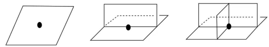
In this work the emphasis is more on semi-flows rather than on flows. Very recent papers show a renew of interest in this kind of dynamics (see [11] and the references cited therein). Considering non-singular semi-flows on dynamical 2-complexes as introduced in [9], one will take advantage of the combinatorial nature of these objects to give an effective criterion for the existence of cross-sections to the semi-flows and flows constructed by means of these complexes. Roughly speaking, the dynamical 2-complexes are special polyhedra (see
[12] - these are polyhedra whose points admit neighborhoods of certain types, illustrated in figure 1) equipped with an orientation of the 1-cells satisfying two simple combinatorial properties. These conditions of orientation of the 1-cells allow to define non-singular semi-flows on these 2-complexes, by giving in some sense the orientation of the semi-flow in a neighborhood of the 1-skeleton. These semi-flows are called combinatorial semi-flows. The criterion of existence of cross-sections we establish here relies on the existence of certain non-negative cocycles in C1(K; Z), namely nice non-negative cocycles (see definition 5.1).
The search of these cocycles is done by searching for the non-negative integer solutions of δ1X = 0, where δ1: C1(K; Z) → C1(K; Z) is the first co-boundary operator of the complex. This system is a linear system of equations with integer coefficients, and thus the set of non-negative integer solutions is generated by a finite number of them. This implies the finiteness of our process. Furthermore, the number of equations and unknowns of the above system depends only linearly on the number of 1-cells in the singular set, that is the set of points where the complex is not a manifold. For more details on the effectivity of the given criterion, we refer the reader to [9]: Although this paper deals with an other type of cocycles, the case of nice non-negative cocycles is handled similarly.
Let us now be more precise on our results. For the sake of simplicity and brievety, we did not intent to establish criteria of existence of cross-sections for the whose class of dynamical 2-complexes, but essentially for an important case, i.e. when the dynamical 2-complex admits, in a compatible way, a structure of dynamic branched surface as defined by Christy (see [3]). It is then called a special dynamic branched surface (see definition 3.2). We give here a combinatorial and effective criterion for a dynamical 2-complex to admit such a structure (proposition 3.7). We refer the reader to [9] for a more complete discussion about the relationships between dynamical 2-complexes and dynamic branched surfaces. Let us recall that branched surfaces, introduced by Williams in [19], are 2-complexes equipped with a smooth structure. Dynamic branched surfaces are branched surfaces carrying non-singular semi-flows. They were introduced by Christy for the study of hyperbolic attractors in 3-dimensional manifolds. We refer the reader to [17, 5, 3] among others for basic notions of hyperbolic dynamics. Our result is the following one (section 5):
Theorem 0.1 An efficient semi-flow on a special dynamic branched surface W admits a cross-section if and only if there exists a nice non-negative cocycle u ∈ C1(K; Z). Any
such cocycle defines a cross-section to any efficient semi-flow on W .
Efficient semi-flows form a particular class of combinatorial semi-flows, they are everywhere transverse to the singular set of the branched surface. They so belong to the class of semi-flows on dynamic branched surfaces defined by Christy in [3]. Roughly speaking, in the work of Christy, a dynamic branched surface is obtained from a hyperbolic attractor by cutting along the stable foliation of the hyperbolic flow, and then identifying any two points lying on a same stable segment. One says that the hyperbolic attractor collapses to the dynamic branched surface. In this “embedded case” theorem 0.1 above implies the following corollary (see section 7):
Corollary 0.2 If an hyperbolic attractor in a compact 3-manifold collapses to a special dynamic branched surface, then the corresponding hyperbolic flow admits a cross-section if and only if there exists a positive cocycle u ∈ C1(K; Z). Any such cocycle defines a cross-section to this hyperbolic flow.
Indeed, if a dynamical 2-complex K is the spine ([12]) of a compact 3-manifold MK (this
is a dynamical 2-spine), then, for any combinatorial semi-flow (σt)t∈R+ on K, there is a
non-singular flow (φt)t∈R+ on MK, transverse to ∂MK and pointing inward, which is
semi-conjugated to (σt)t∈R+. The retraction of the manifold onto the complex plays the role
of the semi-conjugacy. This fact is well-known in the context of branched surfaces. Let us observe that the nature of the cocycles involved changes from theorem 0.1, “nice non-negative cocycles”, to corollary 0.2, “positive cocycles”. A positive cocycle is in particular a nice non-negative cocycle, and thus corollary 0.2 sharpens our result in the embedded case. This is due to the fact that the cross-sections we find in theorem 0.1 might miss some positive loops in the singular graph (where “positive” refers here to the orientation put on the edges in the definition of dynamical 2-complex), which are not necessarily homotopic to periodic orbits of the semi-flow in the general case, but which are in the embedded case. These are the so-called “boundary periodic orbits” in the work of Christy (see [5, 3]). We give a proof of corollary 0.2 without using this knowledge on the periodic orbits of hyperbolic flows.
Speaking of cross-sections leads to think to the mapping-torus or suspension operation. This construction, when applied to a homeomorphism of a compact surface with boundary, gives a 3-dimensional manifold, together with a non-singular flow tangent to the bound-ary and admitting a cross-section. In the Appendix (section 8), we show how to define boundary-tangent flows from dynamical 2-spines. We prove that the existence of a positive cocycle again is a necessary and sufficient criterion of existence of cross-section to these flows. Let us observe that this is no more true if, instead of considering boundary-tangent flows, one considers flows transverse to the boundary of the manifold, as in the case of special dynamic branched surface, but the dynamical 2-complex considered is not a dy-namic branched surface.
Acknowledgements: Some of this work comes from the doctoral dissertation of the author, written under the direction of J. Los. During the elaboration of the paper, the au-thor benefited of a European Marie Curie Grant, and is very grateful toward the Centre de Recerca Matem`atica and the Departament de Matem`atiques of the Universitat Aut`onoma de Barcelona, particularly its Dynamical Systems team, for their hospitality.
1
Flat and dynamical 2-complexes
All the complexes considered in this paper will be piecewise-linear and, unless otherwise stated, connected, and compact. The j-skeleton K(j) of a n-dimensional CW-complex K (0 ≤ j ≤ n) is the union of all the cells in K whose dimension is less or equal to j. Let us recall that each i-cell C, 1 ≤ i ≤ n, comes with an attaching-map hC which is a continuous
map from its boundary (this is a (i − 1)-sphere - S0 consists of two points) to the complex. We will not distinguish between the boundary of C and its image in the complex under this attaching-map hC, both denoted by ∂C, but leave to the reader the (easy) task to
know in each occurence what designates the symbol ∂C.
We will denote by Con(X) the cone over a space X, that is the space X × [0, 1], where X× {1} is identified to a single point. Finally, we denote by ∆3 the closed 3-dimensional simplex.
The 0-cells (resp. 1-cells) of a CW-complex are called the vertices (resp. edges) of the complex. If e is an oriented edge, then e is said to be an incoming edge at its terminal vertex t(e) and an outgoing edge at its initial vertex i(e). Let us observe that an oriented
edge e can be both incoming and outgoing at a same vertex, if this edge is a loop. A graph is a 1-dimensional CW-complex.
We call path (resp. loop) in a topological space X a locally injective continuous map from the interval (resp. circle) to X. Let us observe that a loop in a graph, or a path between two vertices in a graph, defines and is defined by a word in the edges of the graph. This word is unique for a path, and unique up to a cyclic permutation for a loop. We will denote by L(p) (resp. F (p)) the last (resp. first) edge intersected by a path p in a graph Γ. A path or loop in Γ is positive (resp. negative) if it is oriented such that its orientation agrees (resp. disagrees) at any point with the orientation of the edges that it intersects.
1.1 Basic definitions
We first recall the notions of standard complex introduced by Casler (see [2] and also [12, 1]), and the derived notion of flat 2-complex (see [9]).
Following [12], we call special 2-polyhedron a piecewise-linear 2-complex satisfying the following property: For any point x ∈ K, there is a neighborhood N (x) of x in K, a neighborhood N (y) of a point y in the interior of Con((∂∆3)(1)), and a homeomorphism hx: N (x) → N (y) such that hx(x) = y.
Let K be a special 2-polyhedron. The singular graph Ksing(1) is the closure in K of the set of points x whose image under hx belongs to an open 1-cell of the interior of Con((∂∆3)(1)).
The set of crossings Ksing(0) is the set of points x of K such that hx(x) is the base of
Con((∂∆3)(1)). We set K(2)
sing = K. The connected components of K (m+1) sing − K
(m) sing, 0 ≤
m ≤ 1, are called the (m + 1)-components of the complex (the 0-components are the crossings).
With this terminology, a standard 2-complex, as defined by Casler, is a special 2-polyhedron whose all 2-components are 2-cells. We will call flat 2-complex a special 2-polyhedron whose 2-components are either 2-cells, annuli or Moebius-bands.
Figure 1: Non-singular and singular points in flat 2-complexes
Remark 1.1 By definition of a special polyhedron K, there is exactly one 2-component of K incident to any turn of edges in the singular graph of K. If (e, e′) is the turn considered,
we will denote by D(e, e′
) this 2-component.
Important: Let K be any flat 2-complex. Then K admits a canonical structure of CW-complex defined as follows: The vertices are the crossings of the CW-complex, together with a set of valency 2-vertices, one for each connected component of Ksing(1) which is a loop without any crossing. The edges are the 1-components of the complex, together with a set of valency 2 edges, one in each 2-component which is not a disc. We will always assume that our flat 2-complexes K are equipped with this canonical structure of CW-complex, and
their singular graph Ksing(1) with the induced structure. In particular, the edges of Ksing(1) are the 1-components of K. This causes no loss of generality for our purpose.
Let K be a flat 2-complex, together with an orientation on the edges of the singular graph. Let C be any 2-component or 2-cell of K. We will say that C contains an attractor (resp. a repellor) in its boundary if there is a crossing v of K and a germ gv(C) of C at v such
that the two germs of edges of Ksing(1) at v contained in gv(C) are incoming (resp. outgoing)
at v. We will say that the crossing v above is or gives rise to an attractor (resp. a repellor) for C (and for the given orientation).
Definition 1.2 A flat dynamical 2-complex is a flat 2-complex K together with an orien-tation on the edges of the singular graph Ksing(1) satisfying the following two properties:
1. Each crossing of K is the initial crossing of exactly 2 edges of Ksing(1) .
2. Any 2-component which is a 2-cell has exactly one attractor and one repellor for this orientation in its boundary. The other components have no attractor and no repellor in their boundary.
A standard dynamical 2-complex is a flat dynamical 2-complex which is also a standard 2-complex.
Lemma 1.3 ([9])
Let K be a flat dynamical 2-complex. The boundary circles of the annulus and Moebius-band components are positive loops in Ksing(1) . The boundary circle of a disc component D decomposes as pq−1 where p and q are two positive paths in K(1)
sing with initial point the
repellor of D and with terminal point its attractor. They are called the ∂-positive paths of D.
p
q
Figure 2: 2-components in a dynamical 2-complex
Remark 1.4 There are two kinds of annulus components in a flat dynamical 2-complex. The annulus components whose orientations of the boundary loops agree are called coher-ent, whereas the others are incoherent annulus components.
We will need the analog, for flat 2-complexes, of the notion of a surface embedded in a 3-manifold. This will be the role played by the r-embedded graphs defined below.
Definition 1.5 A graph r-embedded in a flat 2-complex K is a graph Γ embedded in K transversaly to the singular graph Ksing(1) and such that:
• The vertices of Γ belong to the interior of the edges of Ksing(1) and its edges are disjointly embedded in the 2-components of K.
• If v ∈ V (Γ) belongs to e ∈ Ksing(1) , then there is exactly one germ of edge of Γ at v embedded in each germ of 2-cell of K at e.
See figure 3.
Figure 3: A r-embedding
A graph Γ r-embedded in K is 2-sided if it has a neighborhood homeomorphic to the trivial I-bundle Γ × [−1, 1], with Γ identified to Γ × {0}. One always will assume a 2-sided graph to be transversely oriented.
1.2 Homology of flat 2-complexes
Let us remind that the singular graph Ksing(1) of a flat 2-complex K is always assumed to be equipped with a structure of CW-complex whose 0-cells are the crossings of K, together with a set of valency 2-vertices in the loops containing no crossing, and whose 1-cells are the 1-components of K. Furthermore, these edges and vertices of Ksing(1) are the only edges and vertices of K contained in Ksing(1) .
If Γ is a graph, an integer cocycle of Γ is a collection of integer weigths, positive, negative or null, on the edges of Γ. If K is a flat 2-complex, an integer cocycle of K is a cocycle in C1(K; Z), i.e. an integer cocycle of the 1-skeleton of K such that the algebraic sum of its weights along the boundary of the 2-cells is zero.
Lemma 1.6 ([9])
If K is a flat 2-complex, then any integer cocycle u ∈ C1(K; Z) defines a graph Γu
r-embedded and 2-sided in K. The converse is true.
For each edge e of the 1-skeleton, the value u(e) is the number of vertices of Γu in e,
each with a weight of +1 or −1 according to u(e) > 0 or u(e) < 0. One so obtains a collection of weighted points in the boundary of each 2-cell. These weighted points can be connected by arcs disjointly embedded in the 2-cells and whose transverse orientation agrees (resp. disagrees) at their extremities with the orientation of the corresponding edges of the 1-skeleton if the sign of the considered weighted point is positive (resp. negative). Conversely, any graph r-embedded and 2-sided in a flat 2-complex is easily proved to define an integer cocycle in C1(K; Z). ♦
Definition 1.7 A directed graph Γ is a graph equipped with an orientation on its edges such that any two vertices are connected by a positive path.
A non-negative cocycle in C1(Γ; Z) is an integer cocycle u such that u(e) ≥ 0 holds for
any edge e ∈ Γ.
A non-negative cohomology class of Γ is a cohomology-class c ∈ H1(Γ; Z) such that c(l) ≥ 0 holds for any positive embedded loop l in Γ.
The following lemma is straightforward and explains why we introduced the notion of directed graph.
Lemma 1.8 Let K be a flat dynamical 2-complex. The singular graph of K, equipped with the orientation on its edges which makes K a flat dynamical 2-complex, satisfies that each of its connected components is a directed graph.
Definition 1.9 Let K be a flat dynamical 2-complex.
A non-negative cocycle of K is an integer cocycle u ∈ C1(K; Z) which defines a
non-negative, non-null cocycle of the singular graph Ksing(1) .
A non-negative cohomology class of K is a cohomology-class c ∈ H1(K; Z) which defines a non-negative, non-null cohomology-class of the singular graph Ksing(1) .
Remark 1.10 It might be worth noticing that the notion of negative cocycle, or non-negative cohomology-class, of a flat dynamical 2-complex is required to be non-non-negative only on the singular graph, and not on the whole 1-skeleton.
Any non-negative integer cocycle defines a non-negative cohomology class. The converse is true, as shown by proposition 1.13 below. Let us stress that this proposition, and more precisely its corollary 1.17, plays a crucial role in the proof of our main result (theorem 5.2). Before stating it we need an additional definition.
Definition 1.11 Let Γ be a graph. Let v be any vertex of Γ.
We will call pushing-map µv: C1(Γ; Z) → C1(Γ; Z) the map defined by:
(µv(u))(e) = u(e) if e is any 1-cell which either is not incident to v or is both incoming and
outgoing at v, (µv(u))(e) = u(e)+1 if e is incoming, not outgoing at v, (µv(u))(e) = u(e)−1
if e is outgoing, not incoming at v.
We will denote by µkv the composition of k pushing-maps µv.
Remark 1.12 Clearly, the image of an integer cocycle u of a graph Γ under any pushing-map is an integer cocycle of Γ in the same cohomology class than u. Furthermore, if Γ is the 1-skeleton of a flat dynamical 2-complex K, then the image of an integer cocycle of K under a pushing-map also is an integer cocycle of K in the same cohomology-class.
Proposition 1.13 Let Γ be a directed graph. If u is any integer cocycle of Γ in a non-negative cohomology-class, then some finite sequence of pushing-maps transforms u to a non-negative cocycle in the same cohomology-class.
Proof of proposition 1.13: To prove this proposition, we need first to introduce some terminology. Let T be a tree together with an orientation on its edges. T is a rooted tree if there is exactly one vertex v in T whose all incident edges are outgoing edges. This vertex v is the root of T . The ends of a rooted tree T are the vertices with exactly one
incident edge. These edges are the terminal edges of T (since T is a rooted tree, each terminal edge is an incoming edge at the corresponding end).
Let T = π−1(Γ) be the universal covering of Γ (π is the associated covering-map). This
is an infinite tree. The edges of T inherit an orientation from the orientation of the edges of Γ.
Let u ∈ C1(Γ; Z) be any integer cocycle in a negative cohomology class. If u is a
non-negative cocycle there is nothing to prove. Let us thus assume that u is not a non-non-negative cocycle.
Let e be any edge of Γ such that u(e) < 0. Let e0 be any edge of T with π(e0) = e.
One defines inductively a sequence T0 ⊂ T1 ⊂ · · · ⊂ Ti ⊂ · · · of rooted trees Ti ⊂ T with
root v0, and a sequence of integer cocycles u0, u1,· · · , ui,· · · of C1(Γ; Z) in the following
way:
T0 = e0, u0 = u.
For i = 1, 2, · · ·: Let vi−1
1 ,· · · , vi−1k be a maximal (in the sense of the inclusion) set of
ends of Ti−1 such that:
• π(vji−1) 6= π(vi−1k ) if j 6= k.
• If xj is the terminal edge of Ti−1 incident to vi−1j , then
mj = |ui−1(π(xj))| = max{|ui−1(π(x))| , x is a terminal edge of Ti−1 , π(t(x)) =
π(vji−1)}.
ui= (µm1vi−1 1
◦ · · · ◦ µmk
vi−1k )(ui−1).
Tiis the union of Ti−1with the edges x of T whose initial vertex is one of the ends vi1,· · · , vki
of Ti−1 and such that ui(π(x)) < 0.
Lemma 1.14 Let i ≥ 1 such that Ti−1 is a proper subset of Ti. Then for any positive
path e0e1· · · ei with ej ∈ Tj, for any 0 ≤ j ≤ i, π∗ui(ej· · · ei) < 0.
Proof of lemma 1.14: We proceed by induction on i. For i = 1: Since u0 is in a
non-negative cohomology-class and by assumption π∗u
0(e0) < 0, the edge e0 is not a loop and
thus has distinct initial and terminal vertices. Therefore, since u1 is obtained from u0 by
applying a pushing-map at the terminal vertex of e0, π∗u1(e0) = 0. By construction the
values of ui on the terminal edges of Ti are negative. The assertion is thus satisfied for
i= 1.
Let us assume that it is satisfied until i, that is for any positive path e0e1· · · ei with
ej ∈ Tj, for any 0 ≤ j ≤ i, π∗ui(ej· · · ei) < 0. One wants to prove that this property is
still true at i + 1.
Let us consider a positive path e0e1· · · ei+1. By construction π∗ui+1(ei+1) < 0.
Further-more as for π∗u
1(e0), and since all the ends of Ti have distinct images under π, π∗ui+1(ei)
is zero. Since the cohomology-class of ui is non-negative, and by the hypothesis of
in-duction, the terminal vertex of ei, which is the initial vertex of ei+1, is distinct from all
the initial vertices of e0, e1,· · · , ei. If the terminal vertex of ei is the only end of Ti, this
observation implies π∗u
i+1(ej) = π∗ui(ej) for j = 0, · · · , i−1. The hypothesis of induction,
together with the remarks above on π∗u
i+1(ei) and π∗ui+1(ei+1), allows to conclude. Let
distinct from the image under π of the initial vertices of the ej, j ≤ i, then the conclusion
is obvious. If the image under π of one of these ends is the same than the image of some i(ej), j ≤ i, then the pushing-map µkπ(i(ej)) applied at this vertex increases the value of
ui on ej−1 by k and decreases the value of ui on all the outgoing edges at i(ej), and in
particular on ej, by k. Therefore π∗ui+1(ej· · · ei+1) < 0 still holds. This completes the
proof of the induction, and so the proof of lemma 1.14. ♦
Corollary 1.15 There exists an integer k ≥ 1 such that Tn = Tk and un = uk for any
n≥ k.
Proof of corollary 1.15: We set M the number of vertices in Γ. If TM+1 6= TM then
lemma 1.14 says that π∗u
M+1 is negative on any positive path ej· · · eM+1. Since M + 1
is strictly greater than the number of vertices of Γ, for some integer j, i(ej) = t(eM+1).
Then π(ej· · · eM+1) is a loop l with uM+1(l) < 0. This is a contradiction with the fact
that the cohomology-class of u, and thus of uM+1, is non-negative. The corollary follows.
♦
Lemma 1.16 Let k be the integer given by corollary 1.15.
1. The cocycle uk is non-negative on the edge π(e0) = e.
2. If uk(x) < 0 for some edge x of Γ, then u(x) < 0.
Proof of lemma 1.16: The cocycle u1 is non-negative on the edge π(e0) (see the beginning
of the proof of lemma 1.14. If no non-negative cocycle ui takes a negative value on π(e0),
there is nothing to prove. If some uj satisfies uj(π(e0)) < 0 then Tj is a proper subset of
Tj+1. Since for n ≥ k Tn= Tk, uk(π(e0)) ≥ 0. Item (1) is proved. ♦ ♦
Corollary 1.17 Let K be a flat dynamical 2-complex. Any non-negative cohomology class in H1(K; Z) is represented by a non-negative cocycle in C1(K; Z).
This is a straightforward consequence of proposition 1.13 and of lemma 1.8. It suffices to apply the sequence of pushing-maps given by proposition 1.13 to the 1-skeleton of K. ♦
1.3 Non-singular semi-flows
Definition 1.18 A non-singular semi-flow on a flat dynamical 2-complex K is a one parameter family (σt)t∈R+ of continuous maps of the complex, which depends continuously
on the parameter t, such that σ0 = IdK, σt+t′ = σt◦ σt′, and satisfying the following
properties:
• No point of K is fixed by the whole family.
• It defines a C∞ non-singular flow in restriction to each 2-component.
Definition 1.19 A cross-section to a non-singular semi-flow on a flat dynamical 2-complex is a 2-sided, r-embedded graph which intersects transversaly, positively, and in finite time, all the orbits of the semi-flow.
In what follows, the triangle T denotes the cone, based at the origin (0, 0) of the oriented plane R2, over the interval y = 1 − x, x ∈ [0, 1]. The rectangle R is the square [0, 1] × [0, 1]. The model-flow on T (resp. on R) is the restriction to T (resp. to R) of the non-singular flow on R2 whose orbits are the lines y = µ−x, µ ∈ [0, 1] (resp. the lines x = µ, µ ∈ [0, 1]).
Definition 1.20 A combinatorial semi-flow on a flat dynamical 2-complex K is a non-singular semi-flow on K satisfying the following properties:
1. There is a decomposition of K in a finite number of triangular and rectangular boxes whose boundary-points are pre-periodic under the semi-flow and such that the semi-flow in restriction to each box is topologically conjugate to the corresponding model-flow.
2. The orientation of the semi-flow agrees, in a neighborhood of the singular graph Ksing(1) , with the orientation of the edges of Ksing(1) .
3. In each disc component, an orbit-segment connects the repellor to the attractor.
4. Let X be a 2-component which is either a coherent annulus component or a Moebius-band. Then the semi-flow is transverse to the rays of X and the core of X is a periodic orbit.
Remark 1.21 The orbit-segment which connect in each disc component the repellor to the attractor will be called separating segment. The union of all the separating orbit-segments is a collection of periodic orbits of the combinatorial semi-flow considered. These orbits will be called separating orbits. Each crossing belongs to exactly one separating orbit. In particular, the crossings are periodic under any combinatorial semi-flow.
Lemma 1.22 ([9])
Any flat dynamical 2-complex K carries a combinatorial semi-flow.
We will call properly embedded orbit-segment of a non-singular semi-flow (σt)t∈R+ on a flat
dynamical 2-complex K an orbit-segment of (σt)t∈R+ whose endpoints, if any, are in the
boundaries of some 2-components of K, and which is transverse to these boundaries at these endpoints.
Lemma 1.23 ([9])
Let K be a flat dynamical 2-complex. Any properly embedded orbit-segment of any combi-natorial semi-flow on K is homotopic, relative to its endpoints if any, to a positive path in the singular graph of K.
Proposition 1.24 ([9])
Any non-negative cocycle u ∈ C1(K; Z) of a flat dynamical 2-complex K defines, for any combinatorial semi-flow (σt)t∈R+ on K, a r-embedded graph Γu transverse to (σt)t∈R+.
2
From semi-flows to flows on 3-manifolds
Definition 2.1 A flat n-complex K (n = 1, 2) is the spine of a compact (n + 1)-manifold with boundary MK if there is an embedding i: K → MK and a retraction rMK: MK →
i(K), which is a homotopy equivalence, such that the manifold MK is homeomorphic to
∂MK× [0, 1] quotiented by the equivalence relation (x, t) ∼ (x′, t′) if and only if t = t′ = 0
and rMK(x) = rMK(x′). The fibers rM−1K(x) are (n + 2 − j)-ods centered at x, where j is
the smallest integer for which x ∈ Ksing(j) .
If K is a flat 2-complex, figure 4 shows the pre-image under rMK of a neighborhood in K
of each of the two types of singular points.
Figure 4: Thickening of flat 2-complexes
A flat dynamical 2-complex which is the spine of some compact 3-manifold will be called a flat dynamical 2-spine.
Remark 2.2 At the difference of the standard spines of Casler or the special spines of Matveev, we admit 2-components which are not 2-cells. Thus two non-homeomorphic (n + 1)-manifolds can admit homeomorphic flat 2-spines.
Proposition 2.3 below treats the problem of reconstructing a non-singular flow on the manifold MK from a combinatorial semi-flow on a dynamical 2-spine K.
Proposition 2.3 Let K be a flat dynamical 2-spine of a 3-manifold MK. Then, for any
combinatorial semi-flow (σt)t∈R+ on K, there is a non-singular flow (φt)t∈R+ on MK,
transverse and pointing inward with respect to ∂MK, such that the retraction rMK: MK →
K given by definition 2.1 defines a semi-conjugacy between (φt)t∈R+ and (σt)t∈R+.
Proof of proposition 2.3: Let us consider any maximal (in the sense of the inclusion) orbit-segment Ix contained in some triangular or rectangular box for the semi-flow, where
xis the initial point of Ix. For each point y ∈ rM−1K(x) in the interior of MK, one defines an
interval Iy which projects to Ix under rMK. The glueing of these oriented intervals defines
the orbits of a non-singular flow on MK− ∂MK which is semi-conjugated to (σt)t∈R+ by
rMK. For each point x ∈ K, for each y ∈ r−M1K(x) ∩ ∂M , one now defines an oriented
interval Iy transverse to ∂MK at y and which projects under rMK to Ix. One so completes
the above flow to a non-singular flow on MK which is as anounced. ♦
Remark 2.4 Proposition 2.3 above and remark 2.2 imply that two non-singular flows on two 3-manifolds which are semi-conjugated to a same semi-flow on a same dynamical 2-spine are not necessarily topologically conjugated since their ambient manifolds might be not homeomorphic.
Definition 2.5 A cross-section to a non-singular flow on a compact 3-manifold M3 is a
surface properly embedded in M3, that is with its boundary embedded in ∂M3, and which intersects transversely, positively and in finite time all the orbits of the flow.
Proposition 2.6 With the assumptions and notations of proposition 2.3, any cross-section Γu, u ∈ C1(K; Z), to a combinatorial semi-flow (σt)t∈R+ on K defines a cross-section
Su = r−1MK(Γu) to a flow (φt)t∈R+ on MK semi-conjugated to (σt)t∈R+, as given by
propo-sition 2.3.
Proof of proposition 2.6: The following lemma is straightforward:
Lemma 2.7 Let K be a flat 2-spine of a 3-manifold MK, and let rMK: MK → K be
the retraction given by definition 2.1. Any cocycle u ∈ C1(K; Z) defines a surface S u =
r−1
MK(Γu) properly embedded in MK.
By construction of (φt)t∈R+ (see proposition 2.3), it is clear that, if Γu is a cross-section
to (σt)t∈R+, then the surface Su = rMK−1 (Γu) is a cross-section to (φt)t∈R+. ♦
Remark 2.8 With the assumptions and notations of lemma 2.7, if i: K → MK denotes
the embedding of K in MK and [u] the cohomology class of u in H1(K; Z), then i#([u])
is the cohomology class in H1(MK; Z) associated to Su.
3
Special dynamic branched surfaces
Let K be a flat 2-complex or a graph. A smoothing on K consists of defining at each point of K a tangent space TxK, which depends continuously on x.
When a smoothing is defined on a graph Γ, a tangent line is in particular defined at each vertex v of Γ (we will say that a smoothing is defined at v). There are thus two sides at v. If a smoothing is defined at some vertices of a graph Γ, and p is a path in Γ, one says that p is carried by Γ if p does not cross any turn of edges which are in the same side of a vertex.
When a smoothing is defined along a path p in the singular graph of a flat 2-complex K, it defines two sides with respect to any interval I ⊂ p embedded in K. Since there are three germs of 2-cells incident to each point x of I, two points in two distinct germs at x will be on the same side with respect to x. The corresponding germs are said to be in the locally 2-sheeted side of I at x. The other side is the locally 1-sheeted side of I at x.
Definition 3.1 Let K be a flat dynamical 2-complex, together with a smoothing along a path p in the singular graph Ksing(1) .
This smoothing is compatible with K if, for each embedded interval I ⊂ p, for each crossing v contained in I, exactly two edges in StK(1)
sing
(v) are oriented from the locally 2-sheeted side of I to the locally 1-sheeted side of I.
Definition 3.2 A special dynamic branched surface is a standard dynamical 2-complex which admits a compatible smoothing along its singular graph.
Lemma 3.3 ([3])
Any special dynamic branched surface carries a combinatorial semi-flow transverse to its singular graph S and going at every point of S from the locally 2-sheeted side to the locally 1-sheeted side.
Such a semi-flow is called an efficient semi-flow.
In figure 5, we illustrate what looks like, up to diffeomorphism, an efficient semi-flow in a neighborhood of a crossing of a special dynamic branched surface.
Figure 5: An efficient semi-flow in a neighborhood of a crossing
Definition 3.4 Let W be a special dynamic branched surface.
We will call corner of a positive path (or loop) p in the singular graph of W a crossing v= p(t0) of K in p which is a point of tangency of some efficient semi-flow on W with the
interval [p(t0− ǫ), p(t0+ ǫ)] for ǫ > 0 sufficiently small.
A positive path (resp. loop) without any corner will be called a flat path (resp. a flat loop). A flat positive, immersed loop is called a circuit of W .
Thus, any flat path either is contained in, or contains, a circuit of W . Any flat loop in the singular graph of a special dynamic branched surface W is a circuit of W , or turns k times along a circuit of W .
In the following lemma, we precise, with the above terminology, the form of the 2-components of a special dynamic branched surface. It comes straightforwardly from the work of Christy in [3] and the preceding definitions.
Lemma 3.5 ([3])
If D is any 2-component of a special dynamic branched surface W , then:
1. Each ∂-positive path of D (see lemma 1.3) contains exactly one corner, i.e. ∂D admits exactly two points of tangency x1, x2 with any efficient semi-flow (σt)t∈R+
on W .
2. In particular, ∂D \ {x1, x2} decomposes in two connected components such that
(σt)t∈R+ is incoming in D with respect to one of them and outgoing of D with
respect to the other. In other words, D is in the locally 1-sheeted side of the first connected component, and in the locally 2-sheeted side of the other.
3. The connected component along which (σt)t∈R+ is incoming in D is the union of the
two outgoing edges at some crossing of W , which is the repellor of D.
4. The connected component along which (σt)t∈R+ is outgoing of D is the union of two
flat paths, one in each ∂-positive path of D, from x1 (resp. x2) to the crossing of W
See figure 6. x x1 2 x1 x2 e e e e e e e e e e e e A R R A 1 2 3 4 5 6 6 1 2 3 4 5
Figure 6: A 2-component of a special dynamic branched surface
The definition of an efficient semi-flow on a special dynamic branched surface, together with lemma 3.5 above and classical arguments about symbolic codings lead to the following lemma:
Lemma 3.6 Let W be a special dynamic branched surface and let (σt)t∈R+ be any efficient
semi-flow on W . We call coding train-track τW a train-track embedded in W as follows:
1. There is one vertex in each open edge of the singular graph S. There are two vertices in each 2-component D, one on each side of the separating orbit-segment of (σt)t∈R+
in D.
2. The edges of τW are disjointly embedded in the 2-components and do not intersect
the separating orbit-segments of the semi-flow. Each of these edges connects a vertex in S to a vertex in a 2-component. There are exactly three edges incident to each vertex in S, one in each 2-component of W incident to this point.
3. The smoothing at each vertex in S is the smoothing induced by the smooth structure of the branched surface. The smoothing at a vertex v in a 2-component D is such that the edge connecting v to the locally 1-sheeted side of D is in the locally 1-sheeted side of v.
Then, for any loop carried by a coding train-track τW, there is a periodic orbit of (σt)t∈R+
embedded in a regular neighborhood of τW in W and which projects along the ties of this
neighborhood to the given loop. See figure 7.
Figure 7: Coding train-track
In proposition 3.7 below, we give an effective criterion to check whether or not a given standard dynamical 2-complex is a special dynamic branched surface.
Proposition 3.7 A standard dynamical 2-complex K admits a compatible smoothing along its singular graph if and only if the following two properties are satisfied:
1. No edge in the boundary of any 2-component connects its repellor to its attractor.
2. Each edge e of the singular graph appears exactly once in second position in the union, over all the disc components C, of the ∂-positive paths of C (see lemma 1.3).
Proof of proposition 3.7: Let us first prove the sufficiency of the given conditions. Let e be any edge of the singular graph S. By item (2), there is a ∂-positive path p of some component C in which e appears in second position. Thus e is consecutive in p to an incoming edge e′ at i(e), which occupies the first position in p. From item (2), any
edge e appears exactly once in second position in the set of all ∂-positive paths of disc components. Furthermore, by definition of a dynamical 2-complex, any edge e′ appears
exactly once in first position in this same set. Thus, one can choose an embedding in R2
of a small neighborhood in S of each crossing which satisfies the following property: Let e be any edge of the singular graph. Let p be the ∂-positive path containing e in second position. Let e′ be the incoming edge at i(e) which is consecutive to, and precedes
e in p. Then, e and e′
are adjacent in the cyclic ordering at i(e) induced by the chosen local R2-embedding at this crossing.
There is now a unique way to define a smoothing of the 2-complex in a neighborhood of the crossings which is a compatible smoothing, and such that the tangent plane so defined agrees with the chosen local R2-embedding. The point is to prove that these smoothings can be extended to a compatible smoothing along the singular graph. Let us consider any edge ei1 of Ksing(1) . There is a disc component C with lC = ei1· · · eire−ir+11 · · · e
−1
ir+p, r ≥ 1.
Item (1) implies r > 1. By definition of lC, C is on the locally 1-sheeted side of ei1 at
i(ei1). For the chosen local R
2-embedding, e
i1 and ei2 are adjacent in the cyclic ordering
at t(ei1) = i(ei2). Thus, by definition of the smoothing in a neighborhood of the crossings,
C does not change side along ei1, lying on its 1-sheeted side, and therefore no 2-component
changes side along ei1. The same argument can be applied for any edge of K (1)
sing. Thus, no
germ of 2-component changes side along any edge of the singular graph, and we so have a compatible smoothing along the singular graph of the complex.
Let us now prove the reverse implication of proposition 3.7. The necessity of item (1) is straightforward from the definitions. To prove the necessity of item (2), let us assume that K admits a compatible smoothing along its singular graph. This smoothing defines a local R2-embedding at each crossing of the singular graph. Since a smoothing is defined along each edge, each edge e which is in second position in some ∂-positive path p of a disc component is adjacent, according to the induced cyclic ordering at i(e) = t(e′
), to the edge e′
in first position in p. The conclusion follows. The proof of proposition 3.7 is completed. ♦
4
Periodic orbits of efficient semi-flows
The aim of this section is to prove proposition 4.1 below. This proposition is the main step to prove one implication of our main result (theorem 5.2), that is if some efficient semi-flow on a special dynamic branched surface admits a cross-section, then there exists what we call a nice non-negative cocycle (see definition 5.1).
Proposition 4.1 Any non flat positive loop in the singular graph of a special dynamic branched surface W is homotopic to a periodic orbit of an efficient semi-flow on W .
In a first step, we are going to define a class of positive loops in the singular graph which have the property to be homotopic to periodic orbits of any efficient semi-flow. We will then define elementary homotopies and show that any non-flat positive loop in the singular graph can be transformed to such a loop by a finite sequence of elementary homotopies. Let us recall that, if p is a path, then L(p) (resp. F (p)) denotes the last (resp. first) edge intersected by p. If p′
is an oriented subpath of p, with i(p) = i(p′
) or t(p) = t(p′
), then p− p′
will denote the complementary oriented subpath q of p′
in p, i.e. either p = p′q
or p= qp′.
Definition 4.2 Let l be any positive loop in the singular graph S of a special dynamic branched surface W . The flat pieces of l are the maximal (in the sense of the inclusion) flat subpaths of l, i.e. if c0,· · · , ckare the corners of l, the flat pieces of l are the connected
components f0,· · · , fk of l \ {c0,· · · , ck} with i(fj) = cj = t(fj−1), j ∈ (k+1)ZZ .
In all what follows, the indices to the flat pieces of a given positive loop l will always be considered written modulo the total number of flat pieces in this loop. Thus, if fj is any
flat piece in l, fj+1 (resp. fj−1) is the flat piece following (resp. preceding) fj in l, and
might be equal to fj if there is only one flat piece in l.
Lemma 4.3 Any flat path p in the singular graph S of a special dynamic branched surface W which connects two of the crossings of W admits a unique decomposition p = p1· · · pk,
k≥ 1, such that:
• For i < k, each pi is a flat 2-side (see lemma 3.5) of some 2-component Di,
• The path pk is contained in a flat 2-side of some 2-component Dk,
• The integer k is maximum among the decompositions satisfying the preceding prop-erties.
The subpaths pi (resp. 2-components Di) above are called the characteristic subpaths (resp.
characteristic 2-components) of p. We call characteristic ∂-paths of p the ∂-positive paths qi of the characteristic 2-components Di which are in the complement of the pi in ∂Di.
See figure 8 or 9.
Proof of lemma 4.3: By definition of a dynamical 2-complex, there are two incoming edges e, e′
at the crossing i(p). Exactly one of these two edges, say e′
, is such that e′F
(p) is a flat path. By remark 1.1, there are exactly two 2-component D(e, F (p)), D(e′, F
(p)) incident to the two turns formed by these incoming edges e, e′ with the outgoing edge
F(p). By definition of a flat 2-side, if p1 exists, then it is the flat 2-side h
1 of D(e, F (p))
which follows the edge e. Since each edge appears exactly once in first position in the set of ∂-positive paths, there is no ambiguity. Since p is flat, either p strictly contains h1 or p is contained in h1. In the first case, one takes p1 = h1. One iterates the process
with p′
= p − p1. The process is finite and gives us a decomposition of p satisfying the anounced properties. The unicity of such a decomposition is easily deduced from the above arguments. ♦
Remark 4.4 One proves in the course of the proof of lemma 4.3 that the characteristic 2-components D1,· · · , Dk−1are also uniquely defined, where p = p1· · · pk. However, there is a choice for Dk. One will always consider Dkto be the 2-component D(e, F (pk)), where
e is, as in the proof of lemma 4.3, the incoming edge at i(pk) which forms a corner with
F(pk).
Definition 4.5 The po-length of a flat path in the singular graph of a special dynamic branched surface is the number of its characteristic subpaths minus 1.
The po-length of a positive loop l in the singular graph of a special dynamic branched surface is the sum of the po-lengths of its flat pieces.
The following lemma justifies the introduction of these definitions:
Lemma 4.6 Let W be a special dynamic branched surface. Let l be a positive loop in the singular graph of W which contains at least one corner. If the po-length of l is zero, then any efficient semi-flow on W admits a periodic orbit homotopic to l.
Proof of lemma 4.6: Since po(l) = 0, po(fj) = 0 for any flat piece fj of l. By definition
of the po-length, and with the notations above, for any j, there exists a segment in the boundary of the characteristic 2-component Dj1 (this is the unique characteristic 2-component of fj) connecting L(fj) to L(fj+1). This implies that any coding train-track for
W (see lemma 3.6) carries a loop lτ which decomposes in such segments. Lemma 3.6 gives
then, for any efficient semi-flow (σt)t∈R+ on W , a periodic orbit of (σt)t∈R+ homotopic to
lτ in W . By construction, lτ is homotopic to l, which completes the proof of lemma 4.6.
♦
Definition 4.7 Let l be a non flat positive loop in the singular graph of a special dynamic branched surface. Let f1,· · · , fr be the flat pieces of l. Let fj = fj1· · · f
k(j)
j be the
decomposition of fj in characteristic subpaths given by lemma 4.3.
An elementary homotopy on l at fj consists of substituting the characteristic ∂-path qj1 of
the characteristic 2-component D1
j to the subpath L(fj−1)fj1 of l.
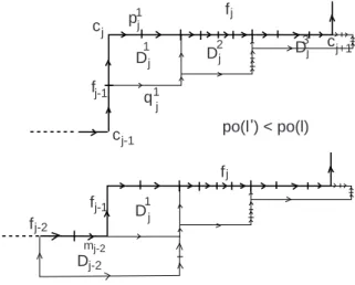
An elementary homotopy at fj is necessary if the po-length of fj is non null.
f f f f fj j j-1 j-1 j-2 pj j j 1 1 1 D D D D D j j 3 2 j-2 mj-2 q j po(l ) < po(l)' c c c j j-1 j+1 1
f
f
f
j j-1 j-2D
1jD
j-2 mj-2po(l') = po(l)
Figure 9: Loops with corners IILemma 4.8 With the assumptions and notations of lemma 4.6,
1. If l′ is the image of l under some necessary elementary homotopy, then l′ is not flat
and po(l′
) ≤ po(l).
2. Let fi, i = 1, · · · , k be the flat pieces of l, and let fi = fi1· · · f k(i)
i be the decomposition
of fi in characteristic subpaths. We denote by l′ the image of l under a necessary
elementary homotopy at fj (which consists of substituting the characteristic ∂-path
qj1 to L(fj−1)fj1 - see definition 4.7).
If po(l′
) = po(l), then:
• The flat piece fj−1 contains exactly one edge.
• There is a natural bijection between the flat pieces fi of l and the flat pieces fi′
of l′
such that f′
j−2 = fj−2F(qj1) and f k(j−2)
j−2 does not contain F (q1j).
See figures 8 and 9.
Proof of lemma 4.8: Since the elementary homotopy that one applies is necessary, the terminal point of the flat subpath of l that one substitutes is not a corner of l. Therefore, by definition of an elementary homotopy, the new loop l′
admits a corner at this point, and thus is not flat.
One applies an elementary homotopy to l at fj, and one denotes by l′ the resulting loop.
One distinguishes two cases:
Case I: The flat piece fj−1 contains more than one edge.
Case II: The flat piece fj−1 contains exactly one edge.
We refer the reader to figures 8 and 9.
Let us first consider the case I above, illustrated in the first picture of figure 8. The loop l′
admits two flat pieces more than the loop l. They form the path qj1. The first one consists of a single edge, the edge F (q1
j), where q1j is the characteristic ∂-path given by lemma 4.3.
The second one is then qj1− F (qj1). By definition, po(F (q1j)) = 0 and po(q1j − F (q1j)) = 0. One has then a natural identification between the flat pieces fi of l and the flat pieces fi′
of l′ in l′ − q1
j: Under this identification, the flat piece f ′ j is equal to fj2· · · f k(j) j , where fj = fj1· · · f k(j)
j is the decomposition in characteristic subpaths given by lemma 4.3. Thus,
po(f′
numerotation we use for the flat pieces of l′, there are the two additional flat pieces given
above between f′
j−1and fj′. Since fj−1 contains more than one edge, po(fj−1′ ) ≤ po(fj−1).
The other flat pieces of l are not modified when passing from l to l′, and thus, if i 6= j and
i6= j − 1, then po(f′
i) = po(fi). Therefore, in this case, po(l′) < po(l).
Let us now consider case II (see figure 9). This figure illustrates the natural identification between the flat pieces fi of l and the flat pieces fi′ of l′. As in case I, po(fj′) = po(fj) − 1.
The piece f′
j−1is equal to q1j−F (qj1). Thus po(fj−1′ ) = 0. If i is distinct from j, j −1, j −2,
as in case I, f′
i = fi, hence po(fi′) = po(fi). It remains to compute po(fj−2′ ). By definition
of an elementary homotopy, f′
j−2 = fj−2F(q1j). Therefore, by definition of the po-length,
if pk(j−2)j−2 contains F (qj1), then po(f′
j−2) = po(fj−2). Thus, in this case, po(l′) = po(l) − 1.
In the other case, po(f′
j−2) = po(fj−2) + 1, and thus po(l′) = po(l). This completes the
proof of lemma 4.8. ♦
One can now complete the proof of proposition 4.1. One assumes given some efficient semi-flow (σt)t∈R+ on a special dynamic branched surface W . By lemma 4.6, any non-flat
positive loop l in the singular graph S of W with po(l) = 0 is homotopic to a periodic orbit of (σt)t∈R+. Let us now consider a non-flat positive loop l in S with po(l) 6= 0. One
applies a necessary elementary homotopy to l, say at the flat piece fj+2. One denotes by
l1 the resulting loop. By lemma 4.8, po(l1) ≤ po(l). If po(l1) = po(l) then by lemma 4.8,
item (2) one has a bijection between the flat pieces of l and the flat pieces of l1. Under
this bijection the flat piece fj of l has as image the flat piece fj of l1, equal to fje1for some
edge e1. The edge e1 satisfies that, if one applies all the necessary elementary homotopies along fj, one eventually gets a flat piece reduced to this single edge. In particular, the
po-length of fj is non-zero. One applies an elementary homotopy on l1 at fj. One iterates
the process. Then:
• Either at some step one obtains a loop li with po(li) < po(li−1).
• Or the number of flat pieces remains constant by lemma 4.8. Thus one eventually applies an elementary homotopy at the flat piece fj+2 of a new loop lk1. If this
elementary homotopy does not make decrease the po-length of lk1, then, as at the
first step, the flat piece fj of the new loop is the concatenation of fje1 with a single
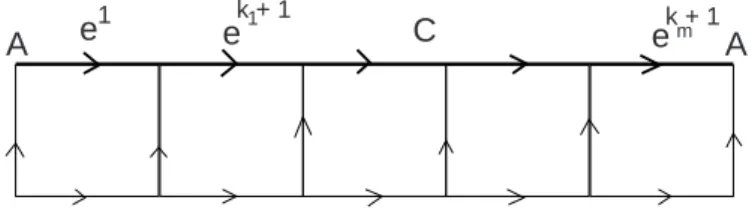
edge ek1+1. Furthermore, always by the same observation than at the first step, the edge e1 is the flat 2-side of some 2-component. By iteration of this process, if
the po-length never decreases, then the finiteness of the singular graph implies the existence of a circuit C = e1ek1+1· · · ekm+1 such that each edge in this circuit is the flat 2-side of some 2-component (see figure 10).
A
A e e C e
k + 1 1
1 k + 1m
Figure 10: An impossible circuit
By definition of a special polyhedron, the circuits of W are trivalent. Since a smooth-ing is defined along the circuits, one so gets the existence of a 2-component in the
locally 2-sheeted side of C which admits C as boundary loop. Since a special dy-namic branched surface admits only disc components and is a dydy-namical 2-complex, this is impossible.
One so obtains a sequence of elementary homotopies which always terminates with a non-flat positive loop ln, homotopic to l in W and such that po(ln) = 0. Together with lemma
4.6, this completes the proof of proposition 4.1. ♦
5
Searching cross-sections
Definition 5.1 A nice non-negative cocycle of a special dynamic branched surface W is a non-negative cocycle u ∈ C1(W ; Z) such that the union of all the positive loops l in the
singular graph for which u(l) = 0 holds is a union of disjointly embedded circuits of W .
This section is devoted to a proof of the following theorem.
Theorem 5.2 Some, and hence any, efficient semi-flow on a special dynamic branched surface W admits a cross-section if and only if there exists a nice non-negative cocycle u∈ C1(K; Z). Any such cocycle defines a cross-section to any efficient semi-flow on W .
Remark 5.3 Theorem 7.3 sharpens theorem 5.2 above in the case where the special dynamic branched surface is the spine of some compact 3-manifold. However, one can construct special dynamic branched surfaces admitting nice non-negative cocycles which are not positive one (see definition 7.2). This forbids to hope to obtain a better criterion in the general case of special dynamic branched surfaces.
5.1 From a nice non-negative cocycle to a cross-section
The following lemma is a straightforward corollary of lemma 3.5 and of the definition of efficient semi-flow in lemma 3.3 (see figure 6).
Lemma 5.4 Any properly embedded orbit-segment of any efficient semi-flow on a special dynamic branched surface is homotopic, relative to its endpoints if any, to a positive path in the singular graph whose number of corners is equal to the number of 2-components intersected by this orbit-segment (there is at least one).
Let us assume the existence of some nice non-negative cocycle u ∈ C1(W ; Z), where W is any special dynamic branched surface. By proposition 1.24, this cocycle defines, for any efficient semi-flow (σt)t∈R+ on W , a r-embedded graph Γu transverse to (σt)t∈R+.
Since u is a nice non-negative cocycle, the intersection-number of this graph Γu with any
positive loop containing at least one corner is strictly positive. By finiteness of the singular graph, lemma 5.4 implies then that any orbit of (σt)t∈R+ will intersect Γu transversely
and positively in finite time. The above r-embedded graph Γu is then a cross-section to
5.2 From cross-sections to nice non-negative cocycles
By definition of a cross-section, proposition 4.1 implies that any integer cocycle u defined by a cross-section to an efficient semi-flow on a special dynamic branched surface W is positive on any non-flat positive loop of the singular graph S. Let us consider the flat loops, that is the embedded circuits. If u is negative on some embedded circuit C, then u is negative on some positive loop Ckp, where p is some positive path in S between two crossings of W , which does not intersect C in its interior, and k is an integer greater than |u(C)u(p)|. The existence of p comes from the fact that any two crossings in S are connected by a positive path. The loop Ckp has at least one corner, at i(p) or t(p), and
u is negative on Ckp. Proposition 4.1 implies then a contradiction with u representing a
cross-section. Therefore, u is non-negative on the embedded circuits of S. One so proved that the cohomology class defined by the cross-section is a non-negative cohomology class. Corollary 1.17 implies then that it is represented by a non-negative cocycle, and, from which precedes, this non-negative cocycle has to be a nice non-negative cocycle. This completes the proof of the missing implication of theorem 5.2.
6
Efficient semi-flows are dilating
In this section, we are interested in the dynamical behaviour of the efficient semi-flows of a special dynamic branched surface. Our result is proposition 6.4 below. This proposition is an intermediate step to prove proposition 7.1 further in the paper, and to eventually obtain a criterion of existence of cross-sections in certain hyperbolic attractors (theorem 7.3).
Definition 6.1 Let W be a special dynamic branched surface.
A path p in W is carried by W if it is transverse to the singular graph S of W and, at each intersection-point x in p ∩ S, crosses both the locally 2-sheeted side and the locally 1-sheeted side of x.
A path p in W is properly embedded if it is an embedded path which does not contain any crossing of W and such that:
• Its endpoints belong to some separating orbit-segment of W .
• For each 2-component C of W , each connected component of p ∩ C intersects exactly once the separating orbit-segment of C.
The combinatorial length l(p) of a properly embedded path p is equal to the number of intersection-points of p with the union of the separating orbits of W minus 1.
Remark 6.2 When speaking of the “number of intersection-points of a path p with the union of the separating orbits”, we mean the number of points in the image of p which also belong to some separating orbit. The combinatorial length of a properly embedded path p is also equivalently defined as the number of intersection-points of the interior of the path with the union of the separating orbits, plus 1, or also the number of 2-components crossed by the path, plus 1.
Definition 6.3 Let W be a special dynamic branched surface. Let (σt)t∈R+ be some
efficient semi-flow on W .
If p is a properly embedded path carried by W , then p is dilated by (σt)t∈R+ if there is
λ >1, C > 0 and t0>0 such that l(σnt0(p)) ≥ Cλ
Proposition 6.4 Let W be a special dynamic branched surface. Let (σt)t∈R+ be some
efficient semi-flow on W .
There exists M > 0 such that, if p is any properly embedded path carried by W , of combi-natorial length greater or equal to M , then p is dilated by (σt)t∈R+.
Let us first notice that the hypothesis for p to be carried by W is necessary in order to have σt(p) a path in W for any time t ≥ 0. Indeed, one required that a path is a locally
injective map from the interval to W . By definition of an efficient semi-flow, this is not the case for σt(p), t any positive real, if p is not carried by W .
Lemma 6.5 With the assumptions and notations of proposition 6.4, let C(p) be the set of points x ∈ p such that there exists tx >0 satisfying that σtx(x) is a crossing of W , for
all t′< t
x, σt′(x) is distinct from the crossings and σt′(x) does not belong to p.
Then the cardinality N (p) of C(p) is finite. If N (p) is strictly greater than the combina-torial length of p, then l(σt1(p)) ≥ l(p) + 1 for some t1>0.
Proof of lemma 6.5: Since W is compact, the number of crossings is finite. By definition, N(p) is lesser or equal to the number of crossings, and thus is finite. Assume now that N(p) is strictly greater than the combinatorial length of p. This implies that there exists at least one point x ∈ p which is not in a separating orbit, but whose image after tx
belongs to a separating orbit. Furthermore, if some point x belongs to a separating orbit, then this remains true for any σt(x), t ≥ 0. Figure 11 illustrates the phenomenom of
dilatation, or non-dilatation when homotoping p along the semi-flow through a crossing. In this figure, α denotes the possible intersections of p with the neighborhood of a crossing, it is important here to recall that p is carried by W . Let tmax be the supremum of all
the times tx for x ∈ C(p). Since N (p) is finite, tmax is finite. From which precedes, the
combinatorial length of σtmax+ǫ(p), ǫ > 0 small, which consists of counting the number of
intersection-points of the interior of the path with the union of the separating orbits, is equal to N (p) ≥ l(p) + 1. This completes the proof of the lemma. ♦
α
α
α
dilated
not dilated
Figure 11: Local dilatation of a properly embedded carried path
Lemma 6.6 With the assumptions and notations of proposition 6.4, There exists t′
2>0 such that any properly embedded loop p carried by W satisfies l(σt2(p)) ≥
l(p) + 1.
Proof of lemma 6.6: Let p be any properly embedded loop carried by W . Let C be any circuit of W intersected by p (there exists at least one). By compacity of W , there exists t′
2 >0 such that any crossing of C is in the image of some σt, t < t′2. If for some t ≤ t′2,
N(σt(p)) > l(p), then l(σt′
2(p)) ≥ l(p) + 1 by lemma 6.5. Let us assume N (σt′2(p)) = l(p).
Then, for any t < t′
neighborhood of any crossing v in C is an arc which intersects in this neighborhood the separating orbit of v. In other words, the intersection of σt(p) with a neighborhood of a
crossing in C is in the case of no dilatation illustrated by figure 11. This implies that none of the two phenomenoma illustrated by figure 12 occurs along any edge in C. That is: Let v be any crossing in C. Let w be the crossing following v in C, and let [vw] an edge in C connecting v to w. If some germ of 2-component at v contains two germs of edges at v which are consecutive in C, then the germ at w to which it is connected through [vw] satisfies this same property. Therefore, there exists a 2-component which is on the locally 2-sheeted side of any point of C, and which contains C in its boundary, that is admits C as boundary circle. By definition of a special dynamic branched surface, the 2-components are discs. And a special dynamic branched surface is in particular a dynamical 2-complex. One so obtains a contradiction with the definition of dynamical 2-complex, which states in particular that, in the boundary of a disc component, there are exactly one repellor and one attractor for the orientation induced by the edges of the singular graph. The proof of lemma 6.6 is completed. ♦ v w v w [vw] [vw]
Figure 12: Never occurs if no dilatation
Corollary 6.7 With the assumptions and notations of proposition 6.4, there exist M > 1 and t2 > 0 such that, if p is any properly embedded path carried by W of combinatorial
length l(p) ≥ jM , j ≥ 1, then l(σt2(p)) ≥ l(p) + j.
Proof of corollary 6.7: Since the singular graph S of W is finite, there exists M > 1 such that if l(p) ≥ M , then some edge of S will contain two points of p. This implies that one can embed a loop b in a small neighborhood of a subpath p′
of p in W , which intersects the same edges of the singular graph than p′
. One proved in lemma 6.6 that there exists t′
2 > 0 such that l(σt′
2(b)) ≥ l(b) + 1. The arguments used precedingly clearly apply to
show that p′
satisfies this same property, i.e. there exists t2 >0, which will be fine for any
path p′ as above, such that l(σ t2(p
′)) ≥ l(p′) + 1 (t
2 is possibly slightly greater than t′2).
Therefore, l(σt2(p)) ≥ l(p) + 1. If l(p) ≥ jM , then p contains at least j distinct subpaths
as the subpath p′
above. Therefore, in this case l(σt2(p)) ≥ l(p) + j. This completes the
proof of corollary 6.7. ♦
Proof of proposition 6.4: By corollary 6.7, there exist t2 > 0 and M > 1 such that, if
p is any properly embedded path carried by W with l(p) = jM + r, r ≤ M − 1, then l(σt2(p)) ≥ l(p)+j. That is l(σt2(p)) ≥ l(p)(1+
1 M)−
r
M. Let us observe that − r M ≥ 1 M−1. Let λ′ = 1 + 1 M and C ′ = 1 M − 1 (C
′ is negative). From which precedes, by definition of a
semi-flow, l(σnt2(p)) ≥ l(p)(λ′ n+ C ′ l(p)(λ ′n−1+ λ′n−2+ · · · + 1)). Since l(p) ≥ M and C′ <0, l(σnt2(p)) ≥ l(p)(λ′ n+C ′ M(λ ′n−1+ λ′ n−2+ · · · + 1)). Since λ′n−1+ λ′n−2+ · · · + 1 = 1−λ′ n 1−λ′ , λ′n+C′ M(λ ′ n−1+λ′ n−2+· · ·+1) = λ′n(1− C′ M(1−λ′))+ C′ M(1−λ′). By definition, C′ M(1−λ′) = 1− 1 M.
Thus C′ M(1−λ′) >0 and 1 − C′ M(1−λ′) >0. This implies l(σnt2(p)) ≥ (1 − C′ M(1−λ′))λ ′nl(p) for
any properly embedded path p carried by W with l(p) ≥ M , where λ′ >1 by definition.
This completes the proof of proposition 6.4. ♦
7
Hyperbolic flows
We show below that, when one is given a special dynamic branched surface W , which is a spine of some 3-manifold MW, then an efficient semi-flow on W will define a hyperbolic
flow on MW. We refer the reader to [17], [5, 3] or [13, 14, 15] among many others for basic
definitions of hyperbolic dynamic.
We show in this section how our criterion of existence of cross-sections on special dynamic branched surfaces gives a criterion of existence of cross-sections to the hyperbolic attractors associated to these branched surfaces (theorem 7.3).
Proposition 7.1 Let W be a special dynamic branched surface which is the spine of some 3-manifold MW. Then any efficient semi-flow on W is semi-conjugated to some hyperbolic
flow on MW.
This proposition relies mainly on “classical” stuff, essentially found in the work of Christy. The difference with the usual setting is the following one: Whereas, usually, branched sur-faces appear as the quotient of hyperbolic attractors, here one is given a particular kind of branched surface and one wants to prove that they allow to reconstruct such attractors. This is why we need proposition 6.4 at the end of the proof of proposition 7.1.
Proof of proposition 7.1: By definition of a special dynamic branched surface, a dif-ferentiable structure is defined at each point of the 2-complex. One can always choose an embedding iW: W → MW which preserves this differentiable structure, and such that
there is a retraction rW: MW → iW(W ) as given by definition 2.1. Let us observe that,
once chosen a maximal atlas (φi, Ui) for MW, one obtains a collection of local embeddings
pi = φi◦ iW in R3 of overlapping open sets Vi = i−W1(Ui∩ iW(W )) which cover W . This
defines a cyclic ordering on the germs of 2-cells at each point x ∈ W . If C is any circuit of W , its lift under r−1W in the boundary of MW contains an embedded closed curve. It
is formed by the extremities of the arms of the triods r−1
W (x), x ∈ C, which lie between,
according to the above cyclic ordering, the two germs of 2-cells which are on the locally 2-sheeted side of x. One collapses each such arm to its extremity in ∂MW, so that the
above embedded closed curve becomes a set of tangency points of the fibers of a new re-traction, denoted by rsW, of MW onto W . By construction, all the fibers rWs
−1(x), x ∈ W ,
are intervals which are transverse at their endpoints to ∂MW, and which admit exactly
one interior point of tangency with ∂MW if x is in the singular graph of W , but is not a
crossing of W , and exactly two such points of tangency if x is a crossing of W .
As in proposition 2.3, once chosen an efficient semi-flow (σt)t∈R+ on W , the retraction rsW
defined above allows to construct a non-singular flow (φt)t∈R+ which is semi-conjugated to
(σt)t∈R+ by rsW. In order to prove that (φt)t∈R+ can be chosen to be a hyperbolic flow, one
has to show that one can define, at each point of the interior of MW, three independent
directions, one tangent to (φt)t∈R+, and the two others such that the flow is contracting
along one and dilating along the other.
One easily defines a combinatorial metric on the fibers of the retraction rs
W such that the