HAL Id: halshs-01190840
https://halshs.archives-ouvertes.fr/halshs-01190840
Preprint submitted on 1 Sep 2015
HAL is a multi-disciplinary open access
archive for the deposit and dissemination of sci-entific research documents, whether they are pub-lished or not. The documents may come from teaching and research institutions in France or abroad, or from public or private research centers.
L’archive ouverte pluridisciplinaire HAL, est destinée au dépôt et à la diffusion de documents scientifiques de niveau recherche, publiés ou non, émanant des établissements d’enseignement et de recherche français ou étrangers, des laboratoires publics ou privés.
Atlantic versus Pacific Agreement in Agri-food Sectors:
Does the Winner Take it All?
Anne-Célia Disdier, Charlotte Emlinger, Jean Fouré
To cite this version:
Anne-Célia Disdier, Charlotte Emlinger, Jean Fouré. Atlantic versus Pacific Agreement in Agri-food Sectors: Does the Winner Take it All?. 2015. �halshs-01190840�
Atlantic versus Pacific Agreement in Agri-food Sectors:
Does the Winner Take it All?
Anne-Célia DISDIER Paris School of Economics
INRA Charlotte EMLINGER CEPII Jean FOURÉ CEPII July 2015
This work has been supported by the French National Research Agency, through the program Investissements d'Avenir, ANR-10-LABX-93-01
G-MonD
Working Paper n°42
Atlantic versus Pacific Agreement in Agri-food Sectors:
Does the Winner Take it All?
∗
Anne-C´
elia Disdier, Charlotte Emlinger and Jean Four´
e
†This version: July 27, 2015
Abstract
Trade liberalization of the agri-food sector is a sensitive topic in both Transatlantic Trade and Investment Partnership (TTIP) and Trans-Pacific Partnership (TPP) dis-cussions. This paper provides an overview of current trade flows and trade barriers. Then, using a general equilibrium model of international trade (the MIRAGE model), it assesses the potential impact of these two agreements on agri-food trade and value added. The results suggest that the US agri-food sectors would gain from both agree-ments while almost all their partners and third countries would benefit less, and might register losses in some sectors. However, the two agreements are not competing, since all the contracting parties’ defensive and offensive interests are complementary. Finally, we show that the Atlantic trade may be impacted by the inclusion of harmonized stan-dards within the Pacific agreement but not by its extension to additional members (e.g. China or India).
Keywords: Mega-trade deals; agri-food; CGE model; Transatlantic Trade and In-vestment Partnership; Trans-Pacific Partnership
JEL: F13; F15; Q17
∗We are grateful to S´ebastien Jean, Lionel Fontagn´e, Houssein Guimbard and GTAP 2015 participants
for their suggestions, and to the European Parliament’s Committee on Agriculture and Rural Development which financed a preliminary version of this paper. Any remaining errors are our owns.
†Anne-C´elia Disdier: PSE-INRA, 48 boulevard Jourdan, 75014 Paris, France. Email:
Anne-Celia.Disdier@ens.fr. Charlotte Emlinger: CEPII, 113 rue de Grenelle, 75007 Paris, France. Email: Charlotte.Emlinger@cepii.fr. Jean Four´e: CEPII, 113 rue de Grenelle, 75007 Paris, France. Email: Jean.Foure@cepii.fr.
Introduction
Preferential trade agreements have proliferated since the beginning of the 2000s. However, until recently, their impact on trade and economic growth has been limited (Erixon, 2013). In 2008, only 16% of world trade benefited from preferential tariffs (WTO, 2011) but things are changing with the emergence of so-called mega-trade deals. Regional openness is becoming a major challenge for many countries, while multilateral liberalization, following the collapse of the Doha round negotiations, is being relegated to the sidelines.
These mega-trade deals are seen as a way to compensate unsuccessful multilateral nego-tiations, to cope with issues not yet tackled by the World Trade Organization (WTO), and to benefit from the dynamic economic growth taking place in some areas (Francois, 2014). They are comprehensive agreements which by integrating markets, often go beyond tariffs. Given their size and ambitions, they are fundamentally different from the old regional trade agreements and are likely to have systemic implications for the world economy (Cernat, 2013; Erixon, 2013). They are setting the framework for future regional and multilateral negotiations whose success (or failure) will shape the future distribution of world trade flows. The Transatlantic Trade and Investment Partnership (TTIP) and Trans-Pacific Partner-ship (TPP) currently under negotiation are perfect illustrations of these mega-trade deals. First, they involve countries that respectively represent 46% and 39% of world GDP. Second, they aim at removing trade barriers in a wide range of sectors to ease the exchange of goods and services between partners. The TTIP involves the United States (US) and the European Union (EU), and deals with the removal of the remaining tariffs, and the harmonization of non-tariff measures (NTMs), while the TPP currently includes the US and 11 other countries and focuses mainly on tariffs. Policy makers have huge expectations of both agreements. On November 14, 2009, President Obama committed the US to engaging “with the TPP coun-tries with the goal of shaping a regional agreement that will have broad-based membership and the high standards worthy of a 21st century trade agreement” (Fergusson et al., 2015). Shortly after the launch of the TTIP negotiations on February 13, 2013, European Commis-sion President Barroso declared “A future deal will give a strong boost to our economies on both sides of the Atlantic” (Barroso, 2013).
countries are open questions. For the TTIP and TPP countries, the cost of a non-agreement is not simply the status quo in terms of trade but potentially could result in isolation from dynamic markets, especially in the context of a successful concurrent agreement. Similarly, both agreements may indirectly affect third countries. Although it has no official status in the TPP negotiations, China is very important to the negotiations.1 Anticipating the potential
consequences of a TPP deal for the economy, the Chinese authorities has begun to focus more closely on the on-going discussions, and may join future negotiations.
While these agreements involve the whole economy, in some sectors and in relation to some services the negotiations are rather sensitive. Despite the relatively small share of agri-culture in global output and employment, it is a definite hot topic.2 The issues being raised relate to anxieties over food security, food safety, and poorer health and environmental stan-dards. Cultural differences can also complicate the TTIP negotiations in agri-food sectors. In relation to risk management, Europeans advocate the precautionary principle, and worry about the ‘risk proven approach’ generally favored by the US. At the same time, due to the current level of protection, agri-food flows across TTIP and TPP countries are relatively weak compared to exchanges of manufactured goods, and significant trade potentials exist.
This paper provides a simulation of the trade and welfare impacts that might be expected from these mega-trade deals. We focus on the agri-food sectors,3 which makes a computable general equilibrium model (CGE) appropriate. The analysis will allow us to highlight the sector effects of trade deals, and the global interactions between markets. We rely on the CGE model MIRAGE.4This model has several significant features compared to other models in the
literature. In a nutshell, it comprises a refined baseline (including sector-specific assumptions about total factor productivity, with a specific treatment for agri-food) and it interacts with the Market Access Map (MAcMap) database defined at the 6-digit level of the Harmonized System (HS) allowing for refined modeling of tariffs and trade liberalization scenarios.
1This fact is well understood by the US. In his State of the Union address on January 20, 2015, President
Obama restated the significance of the TPP and TTIP negotiations for the US, underlining the benefits for the US of writing the trade rules rather than leaving this task to others (e.g. China) http://www.whitehouse. gov/the-press-office/2015/01/20/remarks-president-state-union-address-january-20-2015.
2Cultural and audiovisual services are also sensitive and currently are excluded from the TTIP
negotia-tions.
3Agri-food sectors include products covered by the WTO Agreement on Agriculture plus fish and fish
products.
Our contributions to the existing literature on quantification of the effects of mega-deals, and more precisely on the TTIP and TPP, are fourfold. First, our paper provides a detailed assessment of the impact of these two agreements on agri-food trade. Based on the current set of negotiating countries, these agreements cover 12% of world agri-food trade flows in 2012 (excluding intra-EU trade). The impact is further decomposed by negotiating country and sector.
Second, CGE simulations require the use of accurate measures of trade policies. The agri-food sector continues to be affected significantly by public interventions. For tariff barriers, we rely on the MAcMap-HS6 database which offers a disaggregated, exhaustive, and bilateral measure of the protection applied by importing countries on each product. It includes tariff preferences, tariff rate quotas, and ad valorem equivalents (AVEs) for all non-ad valorem duties. In addition, we estimate AVEs of NTMs. In CGE simulations, harmonization of NTMs translates into a cut in their trade restrictiveness, i.e. in their AVEs. AVEs of NTMs are computed at product level using countries’ notifications to the WTO of sanitary and phytosanitary measures (SPS) and technical barriers to trade (TBT). We rely on the method suggested by Kee et al. (2009), which consists of estimating the trade effects of these NTMs and converting them into AVEs using import demand elasticities.
Third, we contribute to the literature on CGE evaluation of trade deals by introducing more differentiation among countries in terms of NTM effects through aggregation, and departing from the usual assumption that the cost effect of a NTM is a pure efficiency loss. Furthermore, the economy – and especially the agri-food sector – is modeled in as much detail as possible. We consider 31 distinct sectors, of which 17 are related to agri-food products. For our reference scenario, we consider progressive but full phasing out of tariffs, and a 25% cut in NTMs for the TTIP deal. Concerning the Pacific partnership, current negotiations deal mainly with tariff barriers although future discussions might include the harmonization of NTMs. Therefore, the TPP reference scenario simulates progressive but full phasing out only of tariffs.
Fourth, we test the sensitivity of our results by considering different trade liberalization schemes. More precisely, we assume various levels of tariffs and NTM cuts. We also simu-late alternative boundaries for the TPP Agreement: deep integration with harmonization of
NTMs alongside tariff cuts, and broad geographic coverage with additional members such as China, India, and South Korea among others.
Our results suggest first that both agreements might have comparable effects in terms of their magnitude on world agri-food trade flows. It seems also that the US would be the main winner in the agri-food sectors, though an Atlantic deal would be more profitable overall to the US than the Pacific agreement. The US applies lower tariffs than its potential FTA partners on its imports and its production is specialized in sectors facing high NTMs in destination markets. Our results suggest also that the impact of both agreements could be (almost) additive for the US and not competing due to a relatively elastic supply of agri-food products despite the similarity among US offensive interests in the Pacific and Atlantic markets.
In terms of trade diversion, our results show that the Pacific countries have more to lose from the conclusion of an Atlantic-only partnership than does the EU from the achievement of a Pacific-only agreement. This is due mainly to their relative specialization which does not match perfectly with the US market. Finally, the magnitude of the effects could be sig-nificantly affected by the form of the TPP Agreement. While a deeper agreement (including NTM cuts) could significantly reduce EU agri-food exports to the US (price competition is affected more by NTMs than by tariffs), a broader TPP including China and India among other countries would affect EU agri-food exports very little and might even trigger trade increases in some sectors. This last result can be explained by the complementarity in terms of specialization between potential TPP members and the EU.
Our paper is organized as follows. Section 1 provides an overview of current TTIP and TPP negotiations, trade patterns, applied tariffs and NTMs. Section 2 presents the CGE modeling framework, and Section 3 describes the simulation scenarios. Section 4 reports and compares the impacts of the two agreements separately, while Section 5 checks the sensitivity of our results to the simultaneity and characteristics (boundaries and trade liberalization) of the two agreements. The paper concludes in Section 6.
1
Atlantic and Pacific trade patterns
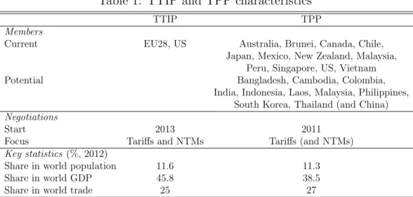
This section describes the main characteristics of the TTIP and TPP trade deals, such as type of negotiation, issues at stake, current trade flows, and protection. As mentioned in the introduction, the main feature of these deals is their huge size (see Table 1). In 2012, TPP members accounted for 11.3% of the world population, 38.5% of world gross domestic product (GDP), and 27% of world trade (import and export). The TTIP area accounted for 11.6% of the world population, 45.8% of world GDP, and 25% of world trade. However, the economic dynamics of these areas show some differences. For example, during the 1970s, 1980s and 1990s, EU-US trade accounted for 40% of world trade (excluding intra-EU trade) but has been decreasing since 2000. On the other hand, the trade flows between TPP countries have increased rapidly since the mid 2000s. Finally, these two agreements cover 12% of world agri-food trade flows in 2012 (excluding intra-EU trade and using the current set of negotiating countries).
Table 1: TTIP and TPP characteristics
TTIP TPP
Members
Current EU28, US Australia, Brunei, Canada, Chile,
Japan, Mexico, New Zealand, Malaysia, Peru, Singapore, US, Vietnam
Potential Bangladesh, Cambodia, Colombia,
India, Indonesia, Laos, Malaysia, Philippines, South Korea, Thailand (and China) Negotiations
Start 2013 2011
Focus Tariffs and NTMs Tariffs (and NTMs)
Key statistics (%, 2012)
Share in world population 11.6 11.3
Share in world GDP 45.8 38.5
Share in world trade 25 27
Note: Key statistics for TPP are computed on the sample of current members. Intra-EU trade is not included. Statistical sources: World Development Indicators for population and GDP; CEPII-BACI database for trade flows.
1.1
Which framework for which negotiations?
Discussions regarding transpacific trade liberalization started in 2002 and involved Chile, New Zealand, and Singapore. The list of participants has expanded over time to include Brunei (2005), the US, Australia, Peru and Vietnam (2008), Malaysia (2010), Canada and
Currently in negociations Potential future members
Legend
Figure 1: Current and potential TPP members
Mexico (2012) and finally Japan (2013), making a total 12 countries currently negotiating mutual market access for their goods and services. Note that this group includes develop-ing, emergdevelop-ing, and industrialized countries. This characteristic (which is not shared by the TTIP Agreement) could influence the pattern and speed of trade liberalization. Current negotiations, which might be concluded in the near future, deal mainly with the dismantling of tariff barriers. In November 2011, TPP countries announced their objective to remove all tariff barriers on trade in goods with the coming into force of the TPP Agreement. It is possible that some adjustment periods might be negotiated for sensitive products, while some tariffs have already been abolished since each of the current negotiating countries is involved in a free trade agreement (FTA) with at least one other TPP partner. Negotiations have begun also on NTMs but are less likely to be concluded in the near future. Current discussions surround ensuring that as tariffs are reduced, they are not replaced by other forms of protection such as NTMs. TPP country coverage may be extended in the future. Several countries including Bangladesh, Cambodia, China, Colombia, India, Indonesia, Laos, Philippines, South Korea, and Thailand, have expressed interest in joining the group (see Figure 1). The potential benefits of TPP membership (or the cost of remaining outside the TPP Agreement) are being recognized increasingly by the Chinese authorities with the result that China is likely to take part in future negotiations.
At first glance, the transatlantic discussions involving just the US and the EU seem more straightforward. The European Commission has a mandate from the EU members to negotiate the TTIP. Negotiations began in 2013 and are expected to be concluded in the near
future. The agreement aims to include the removal of remaining tariffs and the harmonization and/or mutual recognition of regulations and technical requirements (mainly SPS and TBT measures).5 Multiple different rules are costly, and regulatory convergence is one way to reduce these costs. However, this is not always easy, and discussions over specific issues such as public procurement, geographical indications, genetically modified organisms (GMOs), etc. can be complex. If the TTIP Agreement is concluded successfully it should boost trade flows between the two main world economies. EU-US trade relationships are already strong but are being challenged increasingly by other trading countries benefiting or negotiating preferential access to EU and/or US markets (e.g. the recently signed EU-Canada FTA, and the currently being negotiated EU-Japan FTA).
1.2
Trade patterns
6Transatlantic trade relationships already account for a large proportion of world trade. In 2012, flows between the EU and the US represented 4% of world trade. The EU market is the second main destination (after Canada) for US exports, and receives 16% of total US exports (USD 238 billion). At the same time, the US is the main trading partner of EU exporters with 14% of EU exports shipped to the US market annually (USD 353 billion). In terms of imports, the EU is the second most important origin of US imports (16% of total imports), while the US is the third main origin of EU imports (10% of total imports) after China and Russia. Agri-food represents 10% and 8% respectively of US and EU overall exports. In terms of bilateral trade, 9% of US agri-food exports go to the EU and 11% of EU agri-food exports go to the US (Figure 2). Figure 3 shows that transatlantic agri-food trade is concentrated in few sectors: 57% of European exports comprise the beverages and tobacco sector (mainly wine), while beverages and tobacco products, oil seeds, and fruit and vegetables account for half of US exports to the European market.
The TPP area is comparatively very heterogeneous. TPP flows are characterized by the 5In the case of harmonization, a common regulation is defined and applied by both trading partners;
mutual recognition means reciprocal acceptance of each country’s regulation.
6All statistics are computed excluding intra-EU trade flows. These statistics are based on the
BACI database. This database is developed by the CEPII and uses original procedures to harmonize United Nations COMTRADE data (evaluation of the quality of country declarations to average mir-ror flows, evaluation of cost, insurance and freight rates to reconcile import and export declarations, http://www.cepii.fr/CEPII/en/bdd modele/presentation.asp?id=1).
0 20 40 60 80 100 120 140 160 USA Mex. Can. TPP ROW EU Mex. Can.
TPP ROW USA EU Mex. Can.
TPP ROW EU USA Mex. Can.
TPP ROW
EU exports* USA exports Mex. Canada exports Rest of TPP exports
Billion $
ROW: Rest of the World. *Intra-EU trade excluded. EU internal trade is equal to USD 341 billion.
Figure 2: Agri-food exports, by origin and destination in 2012 Note: Authors’ computation using BACI.
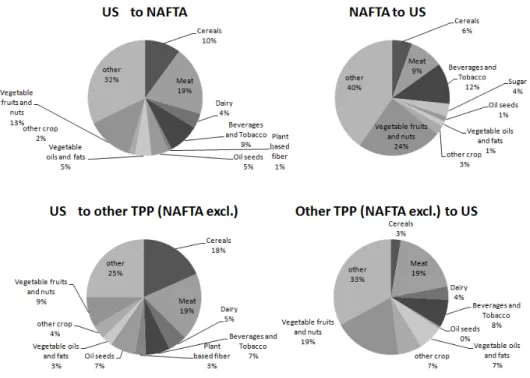
prominence of NAFTA, and the role of Japan. The NAFTA countries are well integrated, and intra-NAFTA flows represent 59% of trade between TPP members (55% for agri-food). Among US world export flows, Canada and Mexico account for 40%. The share in the agri-food sector is lower (27%). The US is also the main export partner for Canada and Mexico, accounting respectively for 73% and 71% of their total exports (68% in agri-food). Japan plays the role of a link between the American and Asian sides of the TPP area. Japan is the second main exporter in the TPP region after the US. Its main export partner is the US (18% of Japanese exports go to the US; by comparison, only 5% of US exports go to Japan). Japan is also an important trading partner for several Asian countries (it accounts for more than 10% of world exports from Brunei, Malaysia and Vietnam), Chile, and New Zealand. TPP countries vary also in the size of their agri-food trade. New Zealand has a strong specialization in agri-food (60% of its total exports), and this sector constitutes more than 15% of Australian and Chilean exports, and around 10% of US and Peruvian exports. The share of agri-food products in exports from Japan and Brunei is very small (less than 1%). Meat, fruits and vegetables and cereals are the main products traded between TPP members (see Figure 4).
Figure 3: Atlantic agri-food trade by sector in 2012 (%) Note: Authors’ computation using BACI.
Figure 4: Pacific agri-food trade by sector in 2012 (%) Note: Authors’ computation using BACI.
1.3
Tariff barriers
Although the tariff barriers affecting transatlantic and transpacific trade have been signifi-cantly reduced over the last few decades some are still in place, especially in agri-food sectors. Table 2 provides some figures extracted from the MAcMap-HS6 database7 jointly developed
by the CEPII and the International Trade Centre (ITC). These data are based on bilateral customs tariffs and include tariff preferences, tariff rate quotas, and AVEs for non-ad val-orem duties which apply to 6% of agri-food tariff lines (compared to 0.6% of industry tariffs). AVEs are aggregated using the reference group method. This alternative weighting scheme reduces the endogeneity problem compared to the classic trade weighted scheme (for more details, see subsection 2.3 and Guimbard et al., 2012).
EU-US bilateral applied protection follows four patterns. First, agri-food imports are better protected than non agri-food imports in both the US and the EU. Average duties on agri-food products are 6.4% in the US and 12.8% in the EU compared to the average protection applied to manufactured goods which is 1.7% in the US and 2.3% in the EU. Second, average EU protection related to US agri-food products is twice as high as the corresponding US protection (12.9% vs. 6.4%). Third, the EU imposes higher duties on a large share of agri-food products: 28.7% of such products (defined at the HS 6-digit level) imported by the EU from the US attract a high tariff (AVE above 15%). The corresponding rate is 6.5% for US agri-food imports from the EU. Fourth, at the sector level, four groups of US agri-food products have high EU tariffs: red meat (bovine, goat, and sheep, average of protection of 75%), dairy (38%), white meat (31%), and sugar (24%), which contrasts with tariffs of less than 5% for oil seeds, plant fibers, oils and fats. The highest levels of protection apply to European sugar at the US border (24%), followed by dairy products (19%). Other EU agri-food sectors are much less affected by US tariffs, with protection at levels below 7%. Within the TPP area, agri-food products attract higher tariffs on average than industry goods (Table 2). However, the level of bilateral protection applied varies widely across coun-tries, and is driven mainly by the existence of FTAs between some country-pairs (Table 3). For example, since the NAFTA, US agri-food tariffs on Mexico and Canada have been very low on average. Tariffs are also low at the US border for agri-food products from Chile, Peru,
and Singapore since the US has in place FTAs with these countries. Similarly, Canadian tariffs vary according to the exporter and the presence of a FTA. Agri-food protection is very low on average for Canadian FTA-partners (Mexico 3.6%, Peru 0.5%) but quite high for other importers (Japan 23%, New Zealand 40%, Singapore 36%) and is 10% for US products. There is a similar disparity in Mexican tariffs which are high for non-FTA partners (Australia 31%, New Zealand 30%, Peru 26%) and low for the US, Chile, and Canada. Among the other TPP members, Australia applies very low agri-food duties on all imports (maximum 2%), while Japan generally imposes high tariffs (except for some countries with whom it has signed an FTA). At sector level, dairy products are affected by high tariffs in several TPP countries. For example, Canada’s average tariff on US dairy products is 110% and on dairy products from other TPP countries is 140%. Cereals are generally well protected. Japanese duties are over 200%, mainly due to the very high levels imposed on rice. Mexican tariffs on cereals are on average 18% for the TPP countries (10% for the US despite the NAFTA). Also, Mexican imports of sugar from other TPP countries (except the US) are subject to a tariff of 97% on average.
Table 2: Average applied protection on transatlantic and transpacific trade, in 2010 (%)
Agri-food Non agri-food
Applied Share Applied Share
protection (%) peaks (%) protection (%) peaks (%) Transatlantic trade
US tariffs applied to EU imports 6.4 6.5 1.7 1.9
EU tariffs applied to US imports 12.9 28.7 2.3 0.9
Transpacific trade
US tariffs applied to TPP imports 2.7 4.8 0.7 0.9
TPP tariffs applied to US imports 7.7 9.0 1.6 7.3
TPP tariffs applied to TPP imports (excl. US) 12.5 10.6 2.1 7.8
Note: Authors’ computation using MAcMap-HS6 database. Tariff peak: AVE above 15%.
1.4
Non-tariff measures
The reduction in tariffs under successive GATT/WTO agreements, and growing concerns among consumers about food safety and quality, has resulted in an increasing role of NTMs in international trade. NTMs are defined as policy interventions other than tariffs which affect the goods trade. Agri-food products are heavily affected by NTMs (UNCTAD, 2005).
Table 3: Average applied protection in agri-food sectors between TPP countries, in 2010 (%)
Importers Partners
Australia Brunei Canada Chile Japan Mala ysia Mexico New Zealand Peru Singap ore Vietnam US Australia . 1.4 1.3 1.0 2.0 0.6 1.3 0.0 1.4 0.0 0.6 0.0 Brunei 2.4 . 3.6 26.5 27.3 4.1 42.8 0.7 14.1 12.1 3.0 6.9 Canada 11.4 62.9 . 4.9 22.9 7.2 3.6 39.9 0.5 36.2 1.4 10.7 Chile 6.1 0.1 2.2 . 2.6 6.0 0.1 3.7 1.5 0.5 6.0 1.2 Japan 32.6 44.9 25.6 12.9 . 5.6 9.9 36.4 8.3 25.9 29.5 21.5 Malaysia 3.3 1.1 3.4 13.0 20.2 . 36.6 1.6 17.9 16.1 21.0 7.9 Mexico 30.7 21.1 3.2 2.6 14.1 9.9 . 29.2 25.9 23.1 10.7 1.0 New Zealand 0.0 0.0 0.2 0.0 2.8 0.9 0.9 . 0.4 0.0 0.7 1.5 Peru 6.0 6.6 2.7 0.8 4.0 2.7 4.6 2.7 . 4.0 4.5 3.4 Singapore 0.0 0.0 1.1 0.0 0.0 0.0 19.0 0.0 0.2 . 0.0 0.0 Vietnam 6.4 4.0 4.7 21.9 20.4 5.2 18.9 6.4 14.9 23.8 . 13.4 US 5.2 9.1 1.4 1.3 6.5 3.0 0.1 6.6 0.5 3.0 2.4 .
Note: Authors’ computation using MAcMap-HS6 database.
Unlike the case of tariffs, the trade and welfare effects of NTMs are ambiguous. The source of this ambiguity is twofold. Firstly, regulations are often necessary to prevent market failure, and to correct negative externalities; however, domestic regulations can be imposed simply to deter imports from foreign competitors (Beghin, 2008). External effects arise when the consumers’ utility (or the producers’ production) is affected by decisions taken by other agents which do not include these externalities in their decision making. For example, pesticides used in production can affect consumers’ health (van Tongeren et al., 2009). Secondly, the implementation process required to comply with NTMs is costly, and may exclude some producers from the market. However, NTMs can contribute to improving market access by enhancing the reputation of foreign products. In such cases, NTMs can act as catalysts for trade.
1.4.1 Descriptive statistics
Our analysis focuses on the two main types on NTMs adopted by TTIP and TPP countries that affect trade flows, namely the SPS and TBT measures. We use the notifications made by these countries to the WTO.8 Each notification provides information on the notifying
8These notifications are used by the WTO in its 2012 World Trade Report (WTO, 2012) and are
avail-able via the Integrated Trade Intelligence Portal (I-TIP) (http://www.wto.org/english/res_e/statis_e/ itip_e.htm). Product codes are often missing from the I-TIP database and were added at the HS 4-digit level by the Centre for WTO Studies of the Indian Institute of Foreign Trade (http://wtocentre.iift.ac.in/).
country (the importer), the affected product (defined at the HS 4-digit level), and the type of measure (SPS vs. TBT). We include all measures notified up to the end of 2012 which means that our dataset is more up to date than that developed by Kee et al. (2009) which was the basis for several previous studies.9 However, WTO members are required to notify only new or changed measures, and the notification requirements apply only to measures which differ from international standards, guidelines, or recommendations, or to situations where no standards exist, and, in addition may have a significant impact on trade. As pointed out in the literature, this could affect the results of an analysis of their trade and welfare impacts. Before we present our descriptive statistics, recall that in almost all cases, NTMs are unilateral measures, i.e. they apply to a given product regardless of its origin. Furthermore, the principle of mutual recognition applies among EU Member States. According to this principle, goods and services can move freely across Member States, and national legislation does not have to be harmonized. Therefore, to avoid bias, we exclude intra-EU trade flows from our NTMs analysis.
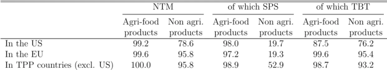
Table 4 provides some statistics on the share of agri-food and non agri-food products (defined at the 6-digit level of the HS classification) affected by at least one NTM, in the US, EU, and TPP countries other than the US. These statistics are further broken down into SPS and TBT measures. A very large share of products is affected by NTMs in these markets; however, our results suggest some differences between agri-food and non agri-food products. TTIP and TPP countries notify SPS and TBT measures on almost all agri-food products. For non agri-food products, the picture is different. For instance, the US notifies fewer NTMs on non agri-food products than the EU and other TPP countries (78.6% vs. 95.8%). Also, NTMs on these products are mainly TBTs. The share of SPS measures notified on non agri-food products is below 20% for the US and the EU and around 50% for the TPP countries (excl. US).
All sectors are affected by NTMs, with coverage ratios (i.e. the share of HS6 lines affected by at least one SPS or TBT within a sector) well above 50%.10 For the US, EU, and TPP
The recent NTM data collected jointly by the World Bank, the UNCTAD and the African Development Bank and available on the WITS (World Bank’s portal for trade data) were not suitable for the present research since country coverage is limited (data are missing for 8 of the 12 TPP countries, including the US).
9Kee et al. (2009)’s NTM data are for year 2004 in the best case (and are likely to be older for some
countries).
Table 4: Share of products affected by at least one NTM, in 2012 (%)
NTM of which SPS of which TBT
Agri-food Non agri. Agri-food Non agri. Agri-food Non agri. products products products products products products
In the US 99.2 78.6 98.0 19.7 87.5 76.2
In the EU 99.6 95.8 97.2 19.3 99.6 95.4
In TPP countries (excl. US) 100.0 95.8 98.9 52.9 98.7 93.2
Note: Authors’ computation using WTO notifications. TPP countries: simple average across countries (US excluded). Agri-food products: Products included in the WTO Agreement on Agriculture plus HS Chapter 3 (fish and fish products).
countries, the coverage ratio is above 95% for all agri-food sectors.
1.4.2 Computation of AVEs of NTMs
We next analyze the impact on trade of the NTMs notified by TTIP and TPP countries. We estimate AVEs, i.e. the level of ad-valorem tariffs that would have an equally trade-restricting effect as the focal NTMs. These AVEs allow comparison between the trade effects of different NTMs and are used in the CGE simulations (see section 2).
To compute the AVEs, we apply the method suggested by Kee et al. (2009). First, we estimate the quantity impacts of NTMs on trade flows, and then convert these effects into AVEs using import demand elasticities computed by Kee et al. (2008). We use the information on NTMs at the HS6 product level, and perform the estimations sector by sector. We define 25 sectors (17 agri-food and 8 non agri-food sectors) which are used also in the CGE simulations. Since the CGE model covers the whole world economy, our sample is extended to include non agri-food activities. Furthermore, third countries are included in addition to TTIP and TPP countries.11 We select all countries notifying NTMs to the WTO,
and collect all measures adopted up to 2012. Our final sample includes 125 countries, and covers 92.5% of world trade flows in 2012. Lastly because of the strong correlation between SPS and TBT – especially for agri-food products where countries often notify both types of measures (see Table 4) – we estimate the global effect of NTMs rather than the respective effects of SPS and TBT.
Our dependent variable, Mrsi, is the dollar value of imports of good i by country s from
country r. We consider only trade flows that are strictly positive in 2012.12 The estimated
11The CGE model also includes services sector, and AVEs for services come from Fontagn´e et al. (2011). 12The absence of bilateral trade between some countries and for some products may be determined by
cross-section trade equation is as follows:
ln Mrsi = a0+ a1tariffrsi+ a2N T Msi+ a3distancers
+ a4cbordrs+ a5clangrs+ F Er+ F Es+ F Ei+ εrsi (1)
where tariffrsi measures the bilateral applied protection on product i, while N T Msi is a
dummy set to 1 if the importing country notifies at least one NTM (SPS and/or TBT) on the product i (0 otherwise). distrs is the bilateral distance between both countries r and
s; cbordrs and clangrs are dummies to control for common border and common language.
F Er, F Es and F Ei are respectively exporter, importer, and product fixed effects. εrsi is the
error term. The country fixed effects incorporate size effects, and also the prices and number of the exporting country’s varieties, the size of demand, and the importing country’s price index. They allow us to avoid the most common mis-specifications in the literature relying on the traditional simplest gravity framework, i.e. lack of control for unobserved relative prices. Baldwin and Taglioni (2006) refer to this as ‘the gold medal of classic gravity model mistakes’, meaning that the bilateral trade costs used as regressors in the estimated equation are correlated with the omitted variable since trade costs enter these unobserved prices.
Our tariff data come from the MAcMap-HS6 database and are for year 2010 (2012 tariffs are not available). NTMs are extracted from the WTO I-TIP database, and our trade data come from the BACI database (cf. supra). Both sets of data are for 2012. Bilateral distance – also from CEPII – proxies for trade costs, and is defined as the sum of the bilateral distances between the countries’ biggest cities weighted by the city populations.13 The dummy variables ‘Common border’ and ‘Common official language’ are extracted from the CEPII database.
Estimations are run sector-by-sector to provide coefficients that reflect the trade effects of NTMs for each sector. The estimated coefficients for the trade restrictiveness of NTMs a2 in
equation (1) are specific to each HS-4 level category, and are constant worldwide. We convert them into importer-HS6 specific AVEs, denoted αs,i using the import demand elasticities εs,i
other aspects than tariffs and NTMs, e.g. endowments, or lack of demand. By focusing on strictly positive flows, we do not attribute these zeros to restrictive tariffs and/or NTMs.
13
provided in Kee et al. (2008):
αs,i=
exp (a2) − 1
εs,i
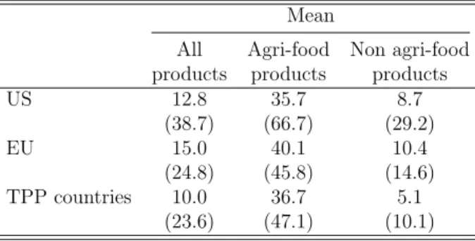
(2) Table 5 reports some of the summary statistics for these importer-HS6 AVEs for the TTIP and TPP countries. First, the mean AVEs are quite high, especially compared to tariffs (Table 2). Second, the breakdown into agri-food and non agri-food products show much higher AVEs of NTMs for agriculture. This (expected) result holds for all countries. The mean AVEs for agri-food products in the US and EU are about four times bigger than the mean AVEs for non agri-food products, and about 7 times bigger in the TPP countries (excl. the US). Third, mean AVEs are slightly higher in the EU than in the US and the TPP countries (excl. US): 15.0% on all products for the EU versus 12.8% for the US and 10.0% for the TPP countries. In a final step, these AVEs will be used in the CGE simulations (cf. section 2).
Table 5: Estimation of AVEs of NTMs: summary statistics, in 2012 (%) Mean
All Agri-food Non agri-food products products products
US 12.8 35.7 8.7 (38.7) (66.7) (29.2) EU 15.0 40.1 10.4 (24.8) (45.8) (14.6) TPP countries 10.0 36.7 5.1 (23.6) (47.1) (10.1)
Note: Mean AVE: simple average across HS6 products. TPP countries: simple average across countries (US excluded). Agri-food products: Products included in the WTO Agreement on Agriculture plus HS Chapter 3 (fish and fish products). Standard deviation across products in parentheses.
Although seemingly large in magnitude, our AVEs for agri-food products are around 10 points lower than those computed by Kee et al. (2009)14: 46.7% for the US, 49.8% for the
EU, and 48.3% for the TPP countries (excl. the US). These differences may be due to the time period covered by the data (2004 for Kee et al. (2009) and 2012 for our data), and the country and product coverage. Our data include some products and several EU and TPP 14AVEs computed by Kee et al. (2009) are available on the World Bank’s website. These elasticities are
countries that are missing from Kee et al. (2009)’s sample.
2
Modeling framework
Evaluating the potential impact of trade agreements on the world economy leads to many issues from tariffs to NTMs which are combined with the medium-term trade pattern dynam-ics. Since a detailed and accurate analysis of all these issues for each sector is impossible, we propose a consistent framework to be applied to all sectors, in order to derive comparative conclusions about the substitutability or complementarity between the Atlantic and Pacific agreements. We use MIRAGE,15 a CGE model of the world economy developed by CEPII
which allows us to include tariffs as well as NTMs that impact on trade in goods and services. While various CGE models have been used to assess the impacts of the Atlantic agreement (Francois et al., 2013; Felbermayr et al., 2013; Bureau et al., 2014) and the Pacific agreement (Petri et al., 2012), none of this work provides a detailed perspective on the agri-food sectors as well as a comparison of the two agreements. This is one of the contributions of our paper.
2.1
On general equilibrium analysis of trade agreements
CGE models have been used frequently to conduct ex-ante assessments of trade agreements. The framework they offer is relevant for a consistent investigation of the interdependences between economies based on trade, and the feedbacks from income effects and factor markets. CGE models have also been applied to analyze how economies react to the new environment following a policy shock. However, these numerical results should be interpreted with caution. Some dimensions of trade agreements (e.g., consequences for employment) are not accounted for in these assessments (see Stanford (2003) on NAFTA Agreement).
The main advantage of the CGE approach is its consistency and exhaustiveness, all world sectors and countries are included in the analysis. However, it is necessary to rely on a sys-tematic methodology which requires some rather strong assumptions. To deal with NTMs, we rely on their AVEs. The very objective of such measures (health and/or environmen-15The version used is nicknamed MIRAGE-e 1.0. A two-page summary of the model is provided in
Appendix .1. The full set of equations is available in the online appendix (http://www.cepii.fr/DATA_ DOWNLOAD/mirage/MIRAGE_Equations_TTIP_TPP.pdf). A technical presentation can be found in Bchir et al. (2002), Decreux and Valin (2007) and Fontagn´e et al. (2013).
tal protection, etc.) cannot be incorporated in the model. Furthermore, some prohibitive measures cannot be explicitly modeled, especially if they are related to only one part of the sector’s output. For instance, we cannot distinguish hormone-fed and hormone-free beef. Nevertheless, we provide a different evaluation which contributes to the modeling literature in two ways. First, we refine the structure of potential costs implied by NTMs by exploiting the information available at the HS-6 digit level, in order to build precise and consistent bilateral AVEs (cf. Section 1.4.2 for their computation). Second, we account for potential externalities related to rent creation due to the presence or imposition of NTMs (and rent reduction due to their harmonization.
2.2
Which impacts apply to which NTMs?
Several authors, for instance Walkenhorst and Yasui (2005) or Fugazza and Maur (2008), point to three different types of trade effects related to NTMs. The first is a direct increase in export costs due to the need to comply with specific requirements and/or to obtain certi-fications required to access the destination country’s market. This is called the “trade-cost” effect. The second corresponds to a “supply-shifting” effect: certain regulations or bans can reduce supply in some sectors. This effect is particularly important in the case of GMOs, or hormone-fed beef. The third effect is a “demand-shifting” effect which occurs when NTM requirements (such as product labeling) affect consumer behavior. The first two effects are trade-impeding, while the demand-shifting effect is ambiguous.
Fugazza and Maur (2008) point to the lack of empirical quantification of a supply-shifting and a demand-shifting effect, and their comment still applies. Fugazza and Maur acknowledge the possibility that TBT measures may change the elasticity of substitution between imported goods, as well as between domestic and foreign goods in the Armington-style demand system. However, they are unable to find estimates of these potential changes. Although these effects might be large, particularly in the case of the TTIP since mutual recognition could be taken as a signal that might shift consumer preferences, we are faced with the same data constraints, and are unable to integrate in our model the supply-shifting and demand-shifting effects.
However, our CGE simulations allow us to address the issue related to the “trade-cost” component of NTMs based on our estimations of NTM AVEs (see Section 1.4.2). Existing
evaluations of trade agreements including NTMs, and of the TTIP and TPP Agreements in particular (Francois et al., 2013; Petri et al., 2012), consider this trade-cost effect as a pure efficiency loss (also called “sand-in-the-wheels”). This makes sense in many cases such as the losses (especially in relation to perishable goods) due to delays incurred by customs procedures. However, this does not cover all the potential cost effects we can expect from implementation of a NTM. In particular, many measures are not neutral regarding income: they can imply a rent that is captured by one or other sides of the border (e.g. the completion of forms at customs implies costs such as wages, or the purchase of logistics services). Furthermore, in the presence of licensing measures, monopolistic rents can benefit local governments (if licences are allocated via auctions), or foreign or local firms (depending on the licence allocation method). Walkenhorst and Yasui (2005) note that these three different ways of considering a cost effect (no rent, rent attributed to locals, rent attributed to foreigners) in our context of perfect competition and a single agent representing consumers and government are equivalent to the implementation of an efficiency loss, an import tax equivalent, or an export tax equivalent.16
The distinction between these cost effects and their equivalent is of prime importance. Their potential impacts on consumers’ real income are different, especially in relation to terms of trade. Andriamananjara et al. (2003) underline that the harmonization of a NTM modeled as an export tax would increase both the terms of trade and the allocation efficiency of the liberalizing country, and thus increase the real income of its consumers. On the other hand, harmonization of a NTM modeled as an import tax equivalent or an efficiency loss would decrease the terms of trade but increase allocation efficiency, leading to an ambiguous effect on consumers’ real income. As already mentioned, previous evaluations of the TTIP and TPP Agreements simply assume that all NTMs have the effect of putting sand in the wheels and skewing the results in one direction. Without further information on these modeling alternatives, our approach remains agnostic; it splits the trade-restrictiveness effect of NTMs into three, allocated as one third to an efficiency loss, one third to generate rent for domestic producers, and one third to rent for foreign producers.
16In our version of the CGE MIRAGE model, this corresponds to an iceberg cost, an additional import
2.3
Data and aggregation
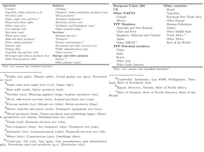
The CGE MIRAGE model is a flexible tool that can be tailored to respond to different policy questions. In the present case, we model the agri-food sector in as much detail as possible. We consider 31 different sectors (16 agri-food industries, 7 manufacturing sectors, 6 services sectors, and 2 energy sectors), and 24 geographical areas (the US, the EU, NAFTA in 2 regions, other TPP members in 5 regions, TPP potential members in 5 regions, and 10 other regions). Detailed aggregations of sectors are provided in Table 6, and of regions in Table 7.
Table 6: Sector aggregation
Agri-food Industry
Cerealsa Clothinge
Vegetable, fruits and nuts (v f) Chemical, rubber and plastic products (crp)
Oil seeds (osd) Metal productsf
Sugar, sugar cane and beetb Transport equipmentg
Plant-based fibers (pfb) Electronic devices (ele)
Other crops (ocr) Machinery and Equipment (ome)
Live animals (ctl) Other manufacturingh
Red meat (cmt) Services
White meat (omt) Business Servicesi
Milk and dairy productsc Transportj
Other animal productsd Finance and insurancek
Forestry (frs) Recreation and other services (ros)
Fishing (fsh) Public administration (osg)
Vegetable oils and fats (vol) Other servicesl
Beverages and tobacco products (b t) Energy and other primary
Other food products (ofd) Energym
Other primary (omn) Note: ’nce’ means ’not classified elsewhere’
a
Paddy rice (pdr), Wheat (wht), Cereal grains nce (gro), Processed rice (pcr).
b
Sugar cane and sugar beet (c b), Sugar (sgr).
c
Raw milk (rmk), Dairy products (mil).
d
Textiles (tex), Wearing apparel (wap), Leather products (lea).
e
Wool, silk-worm cocoons (wol), Animal products nce (oap).
f
Ferrous metals (i s), Metals nce (nfm), Metal products (fmp).
g
Motor vehicles and parts (mvh), Transport equipment nce (otn).
h
Wood products (lum), Paper products and publishing (ppp), Miner-als production nce (nmm), Manufactures nce (omf).
i
Trade (trd), Business services nce (obs).
j
Sea transport (wtp), Air transport (atp), Transport nce (otp).
k
Insurance (isr), Communication (cmn), Financial services nce (ofi).
l
Water (wtr), Construction (cns), Dwellings (dwe).
m
Coal(coa), Oil (oil), Gas (gas), Gas manufacture and distribution (gdt), Petroleum and coal products (p c), Electricity (ely).
Table 7: Country aggregation
European Union (28) Other countries US Brazil Other NAFTA Argentina
Canada European Free Trade Area Mexico Other Europe
TPP Members Russian Federation Australia and New Zealand Turkey
Chile and Peru Other Middle East Singapore, Malaysia and Vietnam North Africab
Japan Other Africa Other ASEANa Rest of the Worldc
TPP Potential members China
India Korea Other Asia Other Latin America
Note: ’nce’ means ’not classified elsewhere’
a
Cambodia, Indonesia, Lao PDR, Philippines, Thai-land, Rest of Southeast Asia.
b
Egypt, Morocco, Tunisia, Rest of North Africa.
c
Rest of Oceania, Rest of North America, Rest of the World.
MIRAGE relies on the Global Trade Analysis Project (GTAP) database for social account-ing matrices (version 8.1). Tariffs are taken from the MAcMap-HS6 database (Guimbard et al., 2012) for years 2007 and 2010, and AVEs for NTMs in goods are our own estimations (see Section 1.4.2). AVEs for NTMs in the service sector are taken from Fontagn´e et al. (2011).
Although we have information on tariffs and NTMs at the HS-6 level (respectively τr,s,iand
complex data. Instead, the model only includes 24 regions and 31 sectors. When aggregating tariffs and AVEs at the country-HS6 level (r, s, i) to the MIRAGE aggregation level (R, S, I), we take advantage of two valuable pieces of information. First regarding NTMs, we consider the contribution of an HS6 line to the aggregate AVE only if at least one NTM is actually implemented in the (r, s, i) trade flow, using the dummy variables δr,s,i constructed from the
WTO notifications. Second, the MAcMap-HS6 database provides information on the weights ωr,s,i of each disaggregated flow which can be used to further aggregate the tariffs and NTMs
from the HS6 to the MIRAGE level. These weights are computed using the reference group method which requires each country to be allocated to one of five world regions (the reference groups) with similar characteristics, using hierarchical clustering analysis. The weight of each flow is the share of good i in the imports of the whole reference group originating from region r, scaled by the size of the imports of country s in its reference group (for more details, see Guimbard et al., 2012). The advantage gained by deriving these weights compared to simply weighting by trade flows is that they take account of at least part of the prohibitiveness of certain transaction costs. Such a measure could completely prevent trade and result in a null contribution to a trade-weighted average but would imply a positive contribution to the reference group weighted aggregate. Letting G(s) denote the reference group of country s, and (ρ, ι) denote the same country-HS6 level as (r, i):
ωr,s,i = Mr,G(s),i P ρ,ιMρ,s,ι P ρ,ιMρ,G(s),ι− P ιMs,G(s),ι (3) aveR,S,I = P
(r,s,i)∈(R,S,I)ωr,s,iδr,s,iαs,i
P
(r,s,i)∈(R,S,I)ωr,s,i
(4)
tariffR,S,I =
P
(r,s,i)∈(R,S,I)ωr,s,iτr,s,i
P
(r,s,i)∈(R,S,I)ωr,s,i
(5)
3
Scenario assumptions
In this section, we present our business-as-usual (BAU) scenario, and the scenarios on which our analysis of the Atlantic and Pacific agreements are based.
3.1
Business-as-usual
Before considering the counterfactual scenarios, a BAU pattern for the world economy which is the “baseline” simulation, is simulated up to 2025. The BAU scenario encompasses two aspects. First, in order to have consistent projections for overall total factor productivity, and trajectories for production factors (labor force, education level, capital accumulation), we rely on macro-economic projections from the EconMap database.17 Second, we take account of
three foreseeable changes to reflect the context of potential Atlantic and Pacific agreements:
Data update MIRAGE base data is for year 2007 only but MAcMap tariff data are avail-able also for year 2010. We therefore implement a linear global tariff update between 2007 and 2010.
The EU For the same reason, we implement completion of the EU28 Single Market on the tariff side (full liberalization of trade flows with the inclusion of Romania and Bulgaria in 2008, Croatia in 2013, and adoption of the EU external tariff by Croatia in 2013).
Known free trade agreements According to the WTO regional trade agreements database,18
since 2007 numerous bilateral agreements have come into force, or been signed and are due to take effect in subsequent years. We counted 100 in-force agreements, 5 signed regional trade agreements (RTAs), and 23 agreements (apart from the TTIP and TPP) currently under negotiation. Our baseline scenario considers the first two categories (“in-force” and “signed”), and implements a simplified version of these agreements. Tariffs are reduced by 100% linearly but at different rates depending on the HS-6 line considered: (i) for half of the products (e.g. less sensitive products, i.e. HS-6 lines with the lowest initial tariffs) tar-iffs are set to zero the year the agreement comes into force ; (ii) for 25% of the remaining products (e.g. less sensitive remaining ones) a linear liberalization in three years time ;and (iii) for the remaining 25% of products (e.g. the most sensitive products, i.e. those with the highest initial tariffs) linear liberalization in five years time.19 Thus, full liberalization 17For a detailed description of the MaGE model, which is used to produce the EconMap database, see
Four´e et al. (2013). The version used is MaGE/EconMap 2.3.
18
RTA-IS available at http://rtais.wto.org, accessed June 2014.
takes place between 2008 and 2013. While this might seem a rather unrealistic assumption, our objective is to prevent our results from attributing to the TPP Agreement the outcomes of already-signed agreements, and including changes in revealed comparative advantage due to these agreements (especially if the EU or the US is involved). This justifies such a basic implementation in our BAU scenario.
The economic impacts of the Atlantic and Pacific agreements are computed as the differ-ence between a path incorporating their enforcement, and this baseline.
3.2
Scenarios for the Atlantic and Pacific agreements
This section reviews the potential outcomes of the Atlantic and Pacific agreements, and provides simulated scenarios. In the case of both agreements, we implement full tariff lib-eralization using the same scheme as in the BAU scenario: HS-6 lines are split depending on their initial tariffs, with differentiated reduction speeds: instant liberalization for half of the lines (the less protected ones), liberalization in three years for a quarter of the remaining lines, and liberalization after five years for the 25% most sensitive lines.20
The Atlantic agreement On the tariff side, we implement full liberalization between 2015 and 2020. The potential outcome in terms of NTMs is less easy to predict. The literature relies on a single evaluation proposed by Ecorys (2009) – 25% reduction in the trade-restrictiveness of NTMs which is not a measure of the potential outcome of negotiations but rather half the reduction that European and American entrepreneurs and regulators think is achievable assuming the political will for its achievement.21 Although this is not completely satisfactory, it is the only information available. Therefore, we assume a 25% cut in the trade restrictiveness of NTMs in our main TTIP scenario. However, we consider that given current opposition to the agreement among civil society, and given the fact that the European Commission has already excluded some topics from the negotiation (e.g. cultural 20In MAcMap-HS6, the applied tariff AVE for a product under a Tariff Rate Quota (TRQ) is the relevant
marginal rate of the TRQ (depending on the quota fill rate). In our scenarios, AVEs for products with TRQs are set to zero, following the scheme for other products. This assumption may have a non-negligible impact on the European beef sector where TRQs are important.
21Ecorys (2009) defines the “Actionability” of an NTM as “the degree to which an NTM of regulatory
divergence can potentially be reduced (through various methods) by 2018, given that the political will ex-ists to address the divergence identified” and mixes business surveys, literature review, sector experts and consultations with EU and US regulators to determine it.
and audiovisual services), the political will may not be sufficient to achieve a 25% cut. We test the sensitivity of our results to a 0% cut, and a 10% cut in NTM trade-restrictiveness.
The Pacific agreement The Pacific agreement is more likely to include a reduction only in tariffs which we implement as full liberalization between 2015 and 2020 in order to maintain symmetry between the Atlantic and Pacific agreements. However, similar to the case of the ASEAN+6 agreements, some NTM provisions may be included in future TPP negotiations. There is also some uncertainty surrounding the final list of country members associated with the Pacific agreement. Some countries have expressed interest in joining the negotiations (Colombia, Indonesia, Laos, the Philippines, South Korea, and Thailand), others have been mentioned as possible candidates (Bangladesh, Cambodia, China, and India). The inclusion of Cambodia, China and India is very likely; Cambodia is a member of ASEAN, and China and India have negotiated FTAs with ASEAN. These two options – inclusion of NTMs (“deep Pacific”) and expansion of TPP country coverage (“broad Pacific”) – are subjected to a sensitivity analysis in subsection 5.2.
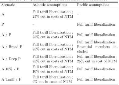
Simulated scenarios We consider seven scenarios, all implemented between 2015 and 2020. The first two scenarios (“A” and “P”) include only one agreement; the remaining five include both the Atlantic and Pacific agreements but involve different assumptions in relation to trade liberalization. The central scenario “A / P” represents a stylized version of both agreements. “A / Broad P” and “A / Deep P” are sensitivity analysis scenarios around the Pacific agreement, and encompass respectively extension of the TPP Agreement to all potential members, and the inclusion of NTMs in the agreement. Finally, “A 10% / P” and “A Tariff / P” model two less ambitious versions of the TTIP Agreement, respectively cutting NTM AVEs by 10%, and excluding NTMs from the negotiations. All scenario assumptions are summarized in Table 8.
The next section presents the results for these scenarios, focusing first on the central assumptions (“A”, “P” and “A / P”), then analyzing the sensitivity of these results to alternative specifications.
Table 8: Summary of alternative scenarios
Scenario Atlantic assumptions Pacific assumptions
A Full tariff liberalization ;
25% cut in costs of NTM –
P – Full tariff liberalization
A / P Full tariff liberalization ;
25% cut in costs of NTM Full tariff liberalization
A / Broad P Full tariff liberalization ;
25% cut in costs of NTM
Full tariff liberalization ;
Potential members
in-cluded
A / Deep P Full tariff liberalization ;
25% cut in costs of NTM
Full tariff liberalization ; 25% cut in cost of NTM
A 10% / P Full tariff liberalization ;
10% cut in costs of NTM Full tariff liberalization
A Tariff / P Full tariff liberalization ;
0% cut in costs of NTM Full tariff liberalization
4
Quantitative results
4.1
US agri-food sectors expand at the expense of their partners
We first identify which countries might gain from signing an agreement. We run separate simulations for the Atlantic and Pacific agreements, i.e. the results reported correspond to the first two scenarios “A” and “P” in Table 8. Table 9 presents the total and agri-food trade variations due to these agreements, and Table 10 presents the country variations in agri-food value added. Our main conclusion is that: In the case of agri-food sectors, the US is the major winner in the context of both the Atlantic and the Pacific agreements. Furthermore, the US’s gains are at the expense of its partners, the majority of which will have to cope with reduced production.
In terms of trade effects, both agreements lead to trade creation for almost all partners. The figures in Table 9 suggest that the Atlantic and Pacific agreements affect overall world trade with comparable orders of magnitude, especially in the case of the agri-food sectors. Our results suggest that the Atlantic and Pacific agreements could lead to respective increases in agri-food trade of USD 30.9 billion and of USD 34.3 billion.
From the US’s point of view, the Atlantic agreement induces higher net export growth than the Pacific agreement. In the case of the Atlantic agreement, US export growth for all sectors reaches USD 149 billion (+29.9%), and USD 35 billion (+159.0%) for agri-food. In the case of the Pacific agreement, the numbers are USD 35 billion (+10.5%) for all sectors
Table 9: Variation in agri-food trade compared to BAU, billion 2007 USD and contribution of agri-food sectors to total variation in trade (pct. points), 2025
Agreement Exporter Importer Agri-food Total Contribution of Agri-food to total (%)
Atlantic EU US 11.6 111.0 10.4
agreement EU -10.1 -48.9 20.7
US EU 34.9 149.2 23.4
Total World 30.9 173.4 17.8
Pacific US Other NAFTA 9.9 3.0 331.3
agreement Other TPP 9.3 32.4 28.9 Other NAFTA US 3.6 7.9 46.2 Other TPP 6.2 8.1 76.9 Other NAFTA 0.5 0.6 95.0 Other TPP US 1.8 21.5 8.2 Other NAFTA 4.3 17.7 24.0 Other TPP -1.2 3.0 -41.7 Total World 30.8 82.2 37.4
Note: Authors’ calculations.
and USD 19 million (+48.6%) for the agri-food sector.
Under the Atlantic agreement, the increase in US agri-food export flows (+159.0%) is much larger than that observed for the EU countries (+55.5%). There are also some trade deflection effects at play between the EU countries. The trade reduction within the EU is quite small in percentage terms (-2.7% in agri-food) but represents more than USD 10 billion. The Pacific agreement also leads to trade creation. The biggest percentage trade increases are observed between Mexico, Canada, and the other TPP countries: +50.6% for Mexican and Canadian exports to other TPP countries, and +94.9% for other TPP countries’ exports to Mexico and Canada. However, in value terms, the biggest increase is for the US exports to Mexico, Canada, and other TPP countries (+USD 19.2 billion). Under the Atlantic agreement, we observe a small trade deflection (-1.1%) across TPP countries excluding the NAFTA countries.
Table 9 shows that the agri-food sector is more sensitive than other sectors to trade liberalization. Agri-food flows exhibit bigger percentage changes than overall flows. However, agri-food generally represents a limited share of total trade gains (11.7% of EU-US trade gains, 24.0% of US-EU gains, and 20.2% of TPP-US gains). US gains under the TPP Agreement are an exceptional case: agri-food gains represent 59.5% of total gains.
In terms of agri-food value added, the pattern is similar for both agreements. While US agri-food value-added increases, in almost all other countries production contracts (Table 10).
The Pacific agreement entails moderate losses for most countries except Canada (-2.7%), which suffers from an erosion of its existing preferential access (due to both initial preferences and the NAFTA Agreement) to the US. Japanese production also faces a decline (-3.4%) concentrated in a few sectors (fruits and vegetables, beverages and tobacco, and other food) where Australia, New Zealand, and the US have strong comparative advantages. Due to this comparative advantage, value added related to agri-food for Australia and New Zealand benefits from the Pacific agreement (+2.5%). New Zealand also gains from the opening of the Japanese and Canadian dairy markets which currently are very protected (respective initial tariffs are 99% and 142%).
The Atlantic agreement scenario results in a decrease in European agri-food value-added (-0.9%). Thus, for the EU, the increase in trade flows is countered by the decrease in intra-EU trade entailed by the agreement. Table 10 shows that the Atlantic agreement has little impact on the value-added of Pacific countries and vice versa.
Table 10: Variation in agri-food value-added, percentage change, 2025
Region Scenarios Atlantic Pacific US 1.1 0.8 EU -0.9 -0.1 Other NAFTA 0.0 -1.4 Canada 0.0 -2.7 Mexico 0.1 -0.6 Other TPP 0.0 -0.5 Chile, Peru -0.1 -0.3
Singapore, Vietnam, Malaysia 0.0 -0.9
Other ASEAN 0.0 -0.3
Japan 0.0 -3.4
Australia, New Zealand -0.1 2.5
Note: Authors’ calculations.
4.2
The differences in the sectoral issues at stake lead to almost
no competition between the agreements
We next conduct a sector analysis of the agreements. The identification of critical sectoral issues allows some conclusions to be drawn on the relative complementarity or substitutability between the Atlantic and Pacific agreements. The results of our analysis could be informative for the US (relative profitability of both agreements) as well as the Atlantic and Pacific
countries (cost of being excluded). We first present the sectoral value-added variations, and extend our conclusions to the aggregate economy. Our results show that the offensive interests of US partners across the Atlantic and across the Pacific differ but their defensive interests are more similar. As a consequence, the potential losses from exclusion from an agreement with the US are limited.
Figure 5: Comparative variation in agri-food value-added due to Pacific and Atlantic agree-ments (pct. variation) and initial agri-food value-added (million 2007 USD), 2025 - TTIP and TPP countries 3 0 0 m illi o n 2 0 0 m illi o n 1 0 0 m illi o n Cereal s Veg etabl e & fr u it Su gar , can e an d b ee t Live A n imal s O the r An im al P ro duct s M ilk & D air y Red M eat W h ite M eat Veget able o il O ther Fo o d Be ve rages an d T o b acco -1 0 1 2 3 4 -4 -2 0 2 4 6 P ac if ic At lan tic USA Ce re als Vegetabl e & fru it Oi l see d s Liv e An im als Ot h er An imal P ro d u cts Red Me at Whi te M eat Vegetabl e o il B ever ag es an d Tob acc o 3 0 0 m illi o n 2 0 0 m illi o n 1 0 0 m illio n -1.0 -0.5 0.0 0.5 1.0 -10 -8 -6 -4 -2 0 2 Pac ifi c Atlanti c EU Cereals Liv e Anim als Mil k & Dair y Red Me at W h ite M e at Ve get able o il Ot h er Fo o d 3 0 0 m illi o n 2 0 0 m illio n 10 0 mil lio n -18 -13 -8 -3 2 -1. 0 -0.5 0.0 0.5 1.0 1. 5 2. 0 Pac ific Atla ntic Oth er NAFT A Ce re als Fiber cro ps Ot her Crops Oth er A n imal P ro d u cts M ilk & D airy Re d M e at White M eat Oth er Fo o d 3 0 0 m illi o n 2 0 0 m illio n 10 0 mil lio n -10 -8 -6 -4 -2 0 2 -0. 4 -0.3 -0. 2 -0.1 0. 0 0.1 0. 2 Pac ifi c Atlanti c Oth er TP P
Note: Authors’ computation. Coordinates on the horizontal axis denote the variation in value-added (pct. points) due to the Atlantic agreement, while coordinates on the vertical axis denote the variation in value-added due to the Pacific agreement. The size of the bubbles denotes the size of value-value-added in the BAU scenario.
Scales differ from one panel to the next. Dotted lines represent the first bisector (where the impact is the same over the two agreements).
Value Added As initial sector protection varies (in terms of both tariffs and NTMs), the impacts of the Pacific and Atlantic agreements are dissimilar across sectors. Figure 5 compares the variation in agri-food value-added induced by both agreements. Coordinates on the horizontal axis denote the variation in value-added (pct. points) due to the Atlantic agreement, while coordinates on the vertical axis denote the variation in value-added due to the Pacific agreement. The size of the bubbles denotes the size of value-added in the BAU scenario. As previously mentioned, the US experiences an increase in its agri-food value added under both agreements. At sector level, white meat, cereals, other animal products, fruits and vegetables, and other food constitute US offensive sectors under both agreements (positive variation in value-added), while red meat and live animals represent an offensive interest only in the Atlantic agreement scenario. The US also has some defensive sectors (negative variation in value-added): dairy, vegetable oils, beverages and tobacco in the Atlantic case, and sugar cane in the Pacific scenario (although this sector does not represent a large share of US agri-food production).
The Atlantic scenario has a negative impact on EU value added in animal products (especially red meat: -8.6%), while vegetable oils, and beverages and tobacco exhibit an increase in EU value added. It is worth noting that only the Pacific agreement has an effect on European white meat value-added due to the competition from Australia and New Zealand in the US market. However, this variation is very small (-0.5%).
In the Pacific agreement scenario, Canada and Mexico are the most affected countries. In the case of both these countries, value added in the red and white meat sectors is positively impacted, while the dairy sector is negatively affected. Note however that these sectors are rather small in terms of their production. The picture is reversed for other TPP countries, where the dairy sector represents an offensive interest (mainly for New Zealand), and the white and red meat value-added is decreasing. Lastly, TPP countries’ agri-food production in dairy, and white and red meat is affected by the Atlantic agreement, but the impact is limited (less than 0.3%).
Given the sector specializations of countries involved in both agreements, the competition effects between the EU and Pacific products on the US market are likely to be unimportant even were both agreements to be implemented simultaneously. However, since US offensive