WORKING
PAPERS
SES
N. 472
VII.2016
How war affects political
attitudes: Evidence from
eastern Ukraine
Martin Huber
and
How war affects political attitudes: Evidence from eastern Ukraine
Martin Huber and Svitlana Tyahlo
University of Fribourg, Department of Economics
Abstract: This study empirically evaluates the impact of the war in eastern Ukraine on the polit-ical attitudes and sentiments towards Ukraine and Russia among the population living close to the war zone on the territory controlled by the Ukrainian government. Exploiting unique survey data that were collected in early 2013 (13 months before the outbreak of the conflict) and early 2015 (11 months after the outbreak), we employ two strategies to infer how the war has affected two differ-ent groups defined by distance to the war zone. First, we apply a before-after analysis to examine intra-group changes in attitudes over time. Second, we use a difference-in-differences approach to investigate inter-group divergence over time. Under particular assumptions, the latter approach yields a lower absolute bound for the effect. We control for a range of observed characteristics and consider both parametric and semiparametric estimation based on inverse probability weight-ing. Our results suggest that one year of conflict negatively affected attitudes towards Russia, while mostly no statistically significant intra- or inter-group differences were found for sentiments towards Ukraine.
Keywords: treatment effect, difference-in-differences, political attitudes, war, conflict, Ukraine, Russia.
JEL classification: P26, D74
We have benefited from comments by Holger Herz, Simon Lapointe, Mickael Melki, Harald Oberhofer, Marco Portmann, Andreas Steinmayr, Dominique van der Walle, and Michael Weber, as well as seminar/conference participants in Fribourg, Zurich, Vienna (University of Economics and Business), Mannheim, Paris (CREST), Xiamen, the Spring Meeting of Young Economists 2016 in Lisbon, and the Annual Meeting of the Swiss Society of Economics and Statistics 2016 in Lugano. Addresses for correspondence: Martin Huber, University of Fribourg, Bd. de P´erolles 90, CH-1700 Fribourg, [email protected]. Svitlana Tyahlo, University of Fribourg, Bd. de P´erolles 90, CH-1700 Fribourg, [email protected]. The collection of the data used in this study was funded by the Grant CR11I1L 135348 “Region, Nation and Beyond. A Transcultural and Interdisciplinary Reconceptualization of Ukraine” of the Swiss National Science Foundation (2013-2015) and the Wolodymyr George Danyliw Foundation
1
Introduction
This study aims at evaluating the impact of the conflict in eastern Ukraine on the political orien-tation of the population in the war-affected area. The pro-Russian unrest in the east of Ukraine, which started in April 2014 shortly after Russia had annexed Crimea in March 2014, escalated to a violent war in spring 2014. Given its geopolitical context and its implications for stability and security in Europe, this military conflict echoed far beyond in multilateral political and economic relations.1 Exploiting unique survey data from a repeated cross section, we investigate how pref-erences about the political status of Ukraine and sentiments towards Ukraine and Russia evolved among individuals living close to the war zone on the Ukrainian-controlled territory between early 2013, i.e. 13 months before the war, and 2015, i.e. 11 months after the war outbreak. Our analysis therefore focuses on the eastern part of Ukraine as far as controlled by government forces, namely Donetsk, Luhansk, Kharkiv, Dnipropetrovsk, and Zaporizhia oblasts (administrative units), which before the war used to share strong cultural and socioeconomic ties. Specifically, these regions represent the most extensively Russian speaking part of Ukraine that had the longest common history with Russia (see Barrington and Herron, 2004).
To infer on the causal effect of the conflict, our empirical strategy relies on the assumption that the intensity of the war decreases in the geographic distance to the war zone. We base our analysis on the minimum road distance by car to the cities of Donetsk or Luhansk - the centers of the self-proclaimed Donetsk and Luhansk People’s Republics, which are both situated close to the front line - as a measure for distance to the war zone. This allows splitting the sample into two treatment groups: all cities located up to 100 km to either Donetsk or Luhansk form the high intensity group, while more distant cities belong to the low intensity group. We employ two econometric approaches. First, we apply a before-after analysis to examine intra-group changes in attitudes over time. This only yields unbiased effect estimates if time trends in attitudes can be ruled out, at least conditional on observed characteristics. Second, our main strategy is based on a difference-in-differences (DiD) approach to investigate inter-group divergence over time. Under particular assumptions (see Fricke, 2015), namely when the impact in the high intensity
1
In response to Russia’s supposed role in the conflict in Ukraine, the European Union (EU) and other countries (e.g. the United States, Canada, Norway, Switzerland, Japan, and Australia) introduced a range of diplomatic and economic sanctions against a list of individuals and companies from Russia and Ukraine. Resorting to countermea-sures, Russia banned food imports from a number of countries. Christen et al. (2015) assess the potential economic consequences of export sanctions between the EU plus Switzerland and Russia.
group weakly dominates that in the low intensity group in absolute terms, a lower bound for the absolute effect of the war on political attitudes is obtained. We control for a range of observed socioeconomic characteristics and consider both parametric and semiparametric estimation based on inverse probability weighting by the propensity score to belong to the high intensity group.
Our findings suggest that the political attitudes towards Russia have deteriorated as a conse-quence of the war. In either group, the before-after differences in (i) supporting a political union with Russia and (ii) stating that Ukraine and Russia should be one state are substantially negative and statistically significant at the 5% level in all but one of our main specifications. Furthermore, for (ii), the DiD approach yields a sizable negative effect which is significant at the 10% level in the majority of specifications. Similarly, a negative DiD estimate is found for the judgment that the Ukrainian and Russian cultures are the same, which is mainly driven by before-after differences in the high intensity group. In contrast, both the before-after and DiD estimates on attitudes and sentiments towards Ukraine and Ukrainians (i.e. sympathy for Ukraine and self-association with other Ukrainians) were insignificant in most cases. The estimated effects are relatively robust to the choice of control variables and the definition of the treatment groups in terms of distance to the war zone.
Among the growing literature investigating the political impacts of exposure to war and vi-olence, ethnic conflicts in Sub-Saharan Africa have attracted particular attention. For instance, the results in Bellows and Miguel (2009), Blattman (2009), and Voors et al. (2012) suggest that individuals who personally experienced wartime violence and trauma during civil wars in Africa (Sierra Leone, Uganda, Burundi, respectively) increase their political and civic engagements and community leadership. Also Bateson (2012), who considers a cross section of 70 countries in Latin America, Africa, North America, Europe and Asia, finds that individuals who report that they or their family members have been recent victims of crimes are more politically active than their non-victimized peers. Applying a regression discontinuity-type design to the timing and location of (Afrobarometer) survey interviews in Zimbabwe, Garcia-Ponce and Pasquale (2015) documents that individuals indirectly exposed to political repression self-report higher levels of trust into the state and its institutions. Erikson and Stoker (2011) examine how Vietnam draft lottery numbers randomly assigned according to birth dates influenced the political attitudes of males. Men with low lottery numbers are found to be more antiwar and liberal in their voting behavior than those with high lottery numbers protected from the draft. As one potential mechanism of war,
DellaVi-gna et al. (2014) investigate how exposure to nationalistic cross-border Serbian public radio affects the voting behavior and anti-Serbian sentiment in the post-conflict region of Croatia at the border with Serbia. Employing a DiD and synthetic control approach, ? consider the electoral effects of the terrorist attacks in Madrid and conclude that they shifted the advantage from the conservative to the socialist party in the 2004 congressional election.
Closer related to our research question, Rohner et al. (2013) employ an instrumental variable method to study the civil conflict in Uganda and find that intense violence strengthens within-ethnic group ties, but significantly weakens trust towards other Ugandans. Most relevant for our work is the study by Coup´e and Obrizan (2016), which investigates the effects of violence on political outcomes in two cities of the Donetsk region which were temporarily controlled by the pro-Russian militants. Relying on cross sectional survey data, their results suggest that physical damage is negatively associated with the turnout probability and the likelihood to know local political representatives. Property damage, on the other hand, increases self-reported votes for pro-Western parties and reduces support for Donbass remaining a part of Ukraine or for any compromise with the pro-Russian forces.2
In contrast to the majority of studies that focus on post-violence outcomes, our analysis, like the one by Coup´e and Obrizan (2016), concerns a point in time when the war was still ongoing. However, our study differs from that of Coup´e and Obrizan (2016) in three dimensions. First, the outcome variables considered mostly differ, with the present work having a stronger focus on political attitudes towards Ukraine and Russia and Coup´e and Obrizan (2016) predominantly (but not exclusively) considering election-related questions. Second, Coup´e and Obrizan (2016) rely on observations within a war affected area, while we exploit variation across areas that were and were not exposed to war. Third, while Coup´e and Obrizan (2016) use a single cross section, our repeated cross section allows observing the outcome variables already prior to the conflict and applying a DiD approach in order to tackle confounding related to time-constant unobservables. In addition to an OLS-based implementation, we base DiD estimation on a semiparametric weighting approach, which is more flexible in terms of functional form assumptions than the estimators conventionally used in the empirical literature.
Our findings confirm the general result from previous studies that exposure to war and violence
2
A further empirical study concerned with the conflict in eastern Ukraine is Zhukov (2016), who, however, does not investigate any effects, but rather the triggers of rebel activity. His results suggest that pre-conflict economic ties with Russia are a better predictor for rebel activity than the ethnolinguistic composition of municipalities.
has consequences with respect to political attitudes, albeit the context differs from much of the literature. Specifically, our estimates suggest that the attitude towards Russia has deteriorated as a consequence of the war, which is probably driven by Russia’s perceived role as major proponent of the separatists’ objectives through its politics, media, and likely military support.3 This appears interesting from a political perspective, because it suggests that the conflict did not make eastern Ukrainians more sympathetic towards Russia, at least in the government-controlled areas, as some might have speculated in the light of the close language and cultural ties with Russia. Quite contrarily, Russia appears to have lost political capital in the most Russian speaking part of Ukraine, while no negative effects on attitudes and sentiments towards Ukraine were found. Our results are somewhat in line with the finding of Coup´e and Obrizan (2016) that the experience of property damage decreases the support for the view that the Ukrainian government should compromise with Russia.
The remainder of this paper is organized as follows: Section 2 describes the conflict background. Section 3 discusses the data and the definition of the treatment groups and provides a range of descriptive statistics on outcomes and control variables. Section 4 outlines our econometric approaches based on parametric and semiparametric before-after and DiD estimation and discusses identification issues, such as migration patterns in the region. Section 5 presents the estimated results along with a range of robustness checks. Section 6 provides two placebo tests for our DiD approach. Section 7 concludes.
2
Background and development of the conflict in Donbass
From the night of 21 November 2013 on the “Euromaidan” movement - a wave of public demonstrations - captured major cities of Ukraine starting on Independence Square in Kyiv. It was triggered by the decision of the Ukrainian government to temporally suspend the preparation to signing the Association Agreement with the EU4 due to concerns about the industrial production and relations between Ukraine and members of the Commonwealth of
3
At the annual press conference on 17 December 2015, Vladimir Putin admitted that there were military intelli-gence officers operating in the east of Ukraine. The video is available at: www.theguardian.com/world/live/2015/ dec/17/vladimir-putins-annual-press-conference-live, retrieved 23 April 2016.
4
The Guide to the EU-Ukraine Association Agreement is available at: eeas.europa.eu/images/top_stories/ 140912_eu-ukraine-associatin-agreement-quick_guide.pdf, retrieved 23 April 2016.
Independent States (CIS).5 The initial demand for closer European integration expanded to requests for political change in the country after the failure of the Ukrainian side to sign the Association Agreement at the Eastern Partnership Summit in Vilnius on 28-29 November 2013.6 The situation culminated into the “Revolution of Dignity” in February 2014 as a result of violent fights with fatalities involving protesters, police and unknown shooters. The Ukrainian parliament voted to oust the acting president who finally fled and left the country. The new presidential elections were scheduled for 25 May 2014. In the meantime, the country was run by a temporary government.
On 16 March 2014, the so-called referendum on the status of Crimea7 took place, after the
peninsula had previously been penetrated by armed forces without insignia most likely belonging to the Russian army.8 The Organization for Security and Co-operation in Europe (OSCE) refused
to send observers to the Crimean “referendum” because it was considered to violate the Ukrainian constitution as well as international law.9 As a result of the referendum’s outcome, Russia officially
annexed the peninsular on 18 March 2014.
In Donbass, the pro-Russian unrest escalated to the status of war in early April 2014 following a sequence of events in Ukraine.10 On 7 April 2014, pro-Russian separatists occupied buildings of the Security Service of Ukraine in Donetsk and Luhansk and self-declared the “Donetsk People’s Republic” followed by the “Luhansk People’s Republic” on 27 April 2014.11 In response to the unrest in Donbass, the Ukrainian government launched an “anti-terrorist operation” against the pro-Russian separatists in mid-April. To de-escalate the conflict in Donbass, the representatives of Ukraine, Russia, the US and the EU agreed in Geneva upon dissolving and disarming non-official
5
Reported by Interfax-Ukraine at: en.interfax.com.ua/news/general/176144.html, retrieved 23 April 2016.
6
The Joint Declaration of the Eastern Partnership Summit is available at: www.consilium.europa.eu/uedocs/ cms_Data/docs/pressdata/EN/foraff/139765.pdf, retrieved 23 April 2016.
7Two options were offered to choose from and either differed from the status quo: whether to join
Rus-sia as a federal subject or to restore the Crimean constitution of 1992 which provided greater power to the Crimean government. Reported by The New York Times at: www.nytimes.com/2014/03/15/world/europe/ crimea-vote-does-not-offer-choice-of-status-quo.html?_r=0, retrieved 23 April 2016.
8See for instance the report of “Suomen Sotilas” (Soldier of Finland): https:
//web.archive.org/web/20150330124704/http://www.suomensotilas.fi/en/artikkelit/ crimea-invaded-high-readiness-forces-russian-federation, retrieved 23 April 2016.
9
The OSCE press release is available at: www.osce.org/cio/116313, retrieved 23 April 2016.
10Reported by BBC: www.bbc.com/news/world-middle-east-26248275, retrieved 23 April 2016.
11Reported by the Human Rights Watch at: www.hrw.org/news/2014/09/11/
military formations in the region. However, the pro-Russian rebels insisted on holding referen-dums and continued occupying buildings of the Ukrainian administration.12 On 11 May 2014, the so-called referendums took place on the separatist-held territories to legitimize the self-declared Donetsk and Luhansk People’s Republics.13 Avoiding formal diplomatic recognition, Russia ex-pressed its respect for the outcomes of the “referendums” and its hope for the “civilized imple-mentation” thereof.14 On 24 May 2014, the self-proclaimed republics declared to form a federal union named “Novorosiya”.15 Since the beginning of the war in Donbass, several waves of army mobilization followed across the territories governed by the Ukrainian authorities. Furthermore, the Russian state-controlled media were banned in the government-held part of Ukraine. On 17 July 2014, the world saw the missile-induced crash of the Malaysia Airlines Flight 17 from Amster-dam to Kuala Lumpur in eastern Ukraine. On 27 January 2015, the Ukrainian parliament passed a resolution declaring Russia an aggressor state16 supporting terrorism and blocking activities of the United Nations (UN) Security Council.17
In response to the development of and the supposed role of Russia in the conflict in Donbass, the European Union (EU) and other countries (e.g. the US, Canada, Norway, Switzerland, Japan, and Australia) introduced or expanded from July 2014 on a range of diplomatic and economic sanctions against a list of individuals and companies from Russia and Ukraine. Following intense consultations of the trilateral contact group (Ukraine, Russia, Organization for Security and Co-operation in Europe), the Minsk II protocol of 12 February 201518was agreed upon after the Minsk protocol of 5 September 201419had failed to resolve the conflict in Donbass. The document outlined
12Reported by The Guardian at:
www.theguardian.com/world/2014/apr/18/ukraine-separatists-occupation-geneva-agreement, retrieved 23 April 2016.
13
Two choices were offered: agree or disagree on the independence status of the Donetsk and Luhansk People’s Republics. Reported by The Guardian at: www.theguardian.com/world/2014/may/10/ donetsk-referendum-ukraine-civil-war, retrieved 23 April 2016.
14
Reported by Reuters at: www.reuters.com/article/us-ukraine-crisis-russia-kremlin-idUSBREA4B04O20140512, retrieved 23 April 2016.
15Reported by Russia Today at: www.rt.com/news/161304-donetsk-lugansk-unite-state/, retrieved 23 April
2016.
16
Reported by Unian at: www.unian.info/politics/1036816-ukrainian-parliament-declares-russia-aggressor-state. html, retrieved 23 April 2016.
17
In 2014-2015, Russia vetoed twice draft resolutions of the UN Security Council on the situation in Ukraine. Reported at: research.un.org/en/docs/sc/quick, retrieved 23 April 2016.
18The document is available in Russian only at: www.osce.org/cio/140156, retrieved 23 April 2016. 19
a package of measures for the implementation of the Minsk agreements to successfully reach a lasting ceasefire. On 17 March 2015, the Ukrainian parliament approved a law on the “special status” of certain parts of Donbass which raised broad discussions about its compliance with Minsk II.20 After months of violations, Ukraine and the separatists ultimately decided to respect the ceasefire from 1 September 2015 on. This entailed a considerable reduction in fighting21 and no further territorial changes occurred. In the beginning of 2016, the war was therefore considered by some to be a “frozen conflict”,22yet clashes and casualties continued and lasting peace was still out of reach.
3
Data and treatment definition
Our data come from a representative population survey in Ukraine conducted in February-March 2013 by the sociological institute “Rating” and repeated in March-April 2015 by the company “Socioinform” on behalf of an interdisciplinary research project on regionalism in Ukraine. The sample consists of a repeated cross section with 6000 individual observations per survey year. The first wave includes all 24 oblasts (administrative units) plus the Autonomous Republic of Crimea, while the second wave only covers the territory controlled by the Ukrainian authorities at that time. For this reason, Crimea, which had been annexed by Russia on 18 March 2014, is excluded, as well as those parts of Donetsk and Luhansk oblasts controlled by the pro-Russian separatists. The sampling was based on stratification by gender, age and municipality type. The face-to-face interviews were conducted either in Ukrainian or Russian, as desired by the respondent. Therefore, no misunderstandings related to language issues are to be expected. Interviewers were instructed to emphasize that the survey was carried out for research purposes only and that analyses would be performed anonymously on the aggregate level, in order to minimize mistrust and reluctance to answer politically sensitive questions. Indeed, response rates are rather high as outlined further below.
This study focuses on questions about preferences for the political future of Ukraine, attitudes about Ukrainian-Russian relations and sentiments towards Ukraine and Ukrainians. Respondents
20Reported by Reuters at: www.reuters.com/article/us-ukraine-crisis-status-idUSKBN0MD1ZK20150317,
re-trieved 23 April 2016.
21
See for instance the UN report at: http://www.un.org/press/en/2015/sc12154.doc.htm, retrieved 23 April 2016.
were asked, inter alia, to state their most preferred option out of five mutually exclusive scenarios: Ukraine remains an independent and neutral state, Ukraine enters a large union including Russia, Ukraine splits into separate states, Ukraine joins the EU, Ukraine joins a large union including Central and Eastern European (CEE) states. In our analysis each option is a binary variable which is coded as one if it is picked as preference and zero otherwise. Note that in the results presented in Section 5, the last two options are excluded, as they are not at the center of this paper’s focus on attitudes towards Ukraine and Russia. Furthermore, interviewees were asked to which extent they agree or disagree with the statements that the Ukrainian and Russian cultures are exactly the same, that Ukraine and Russia should form one state, that they love Ukraine and whether they speak about Ukrainians as “we” and not as “they”. The former two questions are evaluated on a point scale from 1 (“fully disagree”) to 7 (“fully agree”) and the latter two are assessed on a scale from 1 (“definitely no”) to 5 (“definitely yes”).
Besides the outcomes of interest, the data also include a range of socioeconomic information about the respondents, namely gender, age, marital status, education, occupation, native language, religion, residence and self-assessed material conditions. To evaluate how the war in eastern Ukraine affected political attitudes and sentiments of the local population, we focus our analysis on the territories controlled by Ukraine sufficiently close to the war zone when the second survey wave took place. Besides the government-controlled parts of the war-affected Donetsk and Luhansk oblasts, the so-called Donbass region, these areas include three further oblasts: Kharkiv, Dnipropetrovsk, and Zaporizhia (hereafter referred to as the “remainder of the east”). Taken together, these five oblasts form the east of Ukraine, which is characterized by a high concentration of native Russian speakers and heavy industry as well as the geographic proximity and historic connections to Russia. Figure 1 illustrates the front line in Donbass end of March to show which parts of the Donetsk and Lugansk regions where under government control at the time of the second survey.
Figure 1: Front line in Donbass as of 31 March 2015
Source: Information Analysis Center of the National Security and Defense Council of Ukraine: www.mediarnbo.org.
Given that the interviewers could reach only areas controlled by the Ukrainian authorities in early 2015 and that the sociological agencies conducting the surveys were different in the two periods, the included cities and villages in eastern Ukraine only partially coincide across the survey waves. To maximize the comparability of observations in 2013 and 2015, our analysis only includes cities that were observed in both periods.23 The evaluation sample consists of 920 observations in 2013 and 1153 observations in 2015 (see Table A1 in Appendix A) and includes 8 municipalities with 380 observations over both periods in Donbass and 19 municipalities with 1693 observations in the remainder of the east.
To assess whether the evaluation sample is representative for the east of Ukraine prior to the war, we test for mean differences in both control and outcome variables across included and excluded observations, separately for Donbass and the remainder of the east in the first wave. The corresponding descriptive statistics and t-tests are presented in Tables A2 and A3 in Appendix
23The data do not contain any villages in Donbass that appear in both waves. To ensure comparability in
municipality size across Donbass and the rest of the east, we therefore also drop villages in the remainder of the east from our evaluation sample.
A. We observe some significant differences in socioeconomic characteristics across groups. The average material conditions and the proportion of marriages or partnership were significantly higher in the excluded observations of Donbass than in the included ones. Compared to the excluded observations in the remainder of the east, the included ones lived on average in significantly larger cities due to dropping villages and in better material conditions, were more likely to have a university degree and to speak Russian as a native language, and more frequently follow the Kyiv Orthodox Church. Concerning the outcome variables, we do not find any significant differences across the included and excluded observations in Donbass. In the remainder of the east, the included observations were on average less pro-Ukrainian and more likely favored the scenario of a split of Ukraine than excluded ones. We therefore bear in mind that in terms of pre-war covariates and outcome variables, our evaluation sample appears to be much more representative for Donbass than for the remainder of the east. However, the latter seems to be only a minor caveat in the context of our quantitative analysis, which focusses on the effect in the war-affected Donbass.
Our DiD approach outlined in Section 4 is based on the assumption that the distance to the war zone determines the intensity of conflict. We expect that the closer individuals live to the conflict area, the higher the “treatment” (i.e. war) intensity should be. Throughout the military conflict in Donbass, the front line has been moving into one or another direction,24but the regional capitals Donetsk and Luhansk have permanently been at or close to the front line. Therefore, we take the minimum road distance (by car) to Donetsk or Luhansk - also the political centers of the self-proclaimed Donetsk and Luhansk People’s Republics - as a measure for distance to the war zone. Figure A1 in Appendix A displays a frequency distribution of the minimum distance. This allows us to define two treatment groups: all cities located within 100 km to either Donetsk or Luhansk form the high treatment group while more distant cities belong to the low treatment group. The former includes five cities in Donbass and the latter covers three Donbass cities (see Table A4 in Appendix A) plus the remainder of the east.
24
The maps of the front line for different dates of the conflict are provided by the Information Analysis Center of the National Security and Defense Council of Ukraine at: www.mediarnbo.org.
Table 1: Mean covariate values by minimum distance to Donetsk or Lugansk
2013 2015
<100 km ≥100 km Difference p-value <100 km ≥100 km Difference p-value City size: <50000 citizens (binary) 0.133 0.168 -0.035 0.824 0.134 0.115 0.019 0.895
(0.149) (0.073) (0.155) (0.147) (0.055) (0.145)
Female (binary) 0.571 0.555 0.017 0.139 0.573 0.563 0.010 0.785 (0.009) (0.007) (0.011) (0.039) (0.009) (0.037)
Age 45.276 45.182 0.095 0.897 46.671 46.055 0.616 0.562 (0.694) (0.354) (0.725) (1.117) (0.251) (1.049)
Secondary specialized education (binary) 0.410 0.382 0.028 0.704 0.427 0.355 0.072 0.076 (0.077) (0.018) (0.073) (0.036) (0.021) (0.039)
University degree (binary) 0.352 0.417 -0.065 0.541 0.463 0.384 0.080 0.210 (0.111) (0.027) (0.105) (0.054) (0.038) (0.062)
Ukrainian native-speaker (binary) 0.058 0.265 -0.207 0.000 0.061 0.221 -0.160 0.011 (0.031) (0.039) (0.047) (0.042) (0.044) (0.058)
Russian native-speaker (binary) 0.404 0.371 0.033 0.780 0.232 0.287 -0.055 0.531 (0.120) (0.038) (0.116) (0.076) (0.052) (0.086)
Moscow Orthodox Church (binary) 0.307 0.173 0.134 0.214 0.506 0.168 0.339 0.037 (0.111) (0.030) (0.105) (0.168) (0.021) (0.154)
Kyiv Orthodox Church (binary) 0.125 0.184 -0.059 0.543 0.051 0.192 -0.142 0.000 (0.101) (0.029) (0.097) (0.017) (0.016) (0.022)
Autocephalous Orthodox Church (binary) 0.159 0.241 -0.082 0.230 0.177 0.357 -0.180 0.140 (0.059) (0.040) (0.067) (0.125) (0.032) (0.118) Working (binary) 0.552 0.569 -0.017 0.714 0.512 0.528 -0.015 0.749 (0.046) (0.019) (0.046) (0.050) (0.014) (0.048) Retired (binary) 0.248 0.249 -0.001 0.941 0.268 0.275 -0.007 0.825 (0.014) (0.015) (0.020) (0.034) (0.009) (0.032) Single (binary) 0.181 0.166 0.014 0.710 0.122 0.141 -0.019 0.416 (0.039) (0.015) (0.039) (0.017) (0.017) (0.023)
Married or in partnership (binary) 0.610 0.634 -0.024 0.731 0.659 0.614 0.044 0.177 (0.073) (0.021) (0.070) (0.023) (0.024) (0.032)
Material conditions 4.867 4.173 0.694 0.002 4.988 5.103 -0.115 0.761 (1: very good, . . . , 7: terrible) (0.205) (0.073) (0.201) (0.394) (0.102) (0.374)
Note: Each variable is averaged over non-missing values. Standard deviations are clustered on the city level and reported in parentheses.
Tables 1 and 2 report means and t-test results for covariates and outcomes of interest across treatment groups in the two periods. It is mostly municipalities with more than 50000 inhabitants that contribute to our sample. Females represent more than 50 percent of observations and the average age of the respondents is 45-47 years. The majority have at least secondary education, follow one of the Orthodox Churches, are employed, and are married or in a partnership. Russian as native language is more common among respondents than Ukrainian. In both waves, we observe significantly more Ukrainian native speakers in the low treatment group compared to the high one. The respondents in the low treatment group reported significantly better material conditions in 2013 but no significant across-group differences are observed in 2015. The low treatment group includes significantly more followers of the Kyiv Orthodox Church and significantly less followers
of the Moscow Orthodox Church compared to the high treatment group in 2015. Furthermore, the proportion of the respondents with secondary specialized education is significantly larger in the latter. With respect to political attitudes, the high treatment group was significantly more pro-Russian than the low one in the first wave. In the second period, however, only the sentiments towards Ukraine remain significantly different across groups.
Table 2: Mean outcome values by minimum distance to Donetsk or Lugansk
2013 2015
<100 km ≥100 km Difference p-value <100 km ≥100 km Difference p-value Independent, neutral state (binary) 0.193 0.347 -0.153 0.048 0.627 0.434 0.193 0.226
(0.073) (0.031) (0.074) (0.153) (0.071) (0.156)
Union with Russia (binary) 0.591 0.397 0.194 0.022 0.119 0.103 0.016 0.856 (0.077) (0.038) (0.080) (0.095) (0.012) (0.088)
Split into separate states (binary) 0.011 0.014 -0.002 0.776 0.102 0.047 0.055 0.265 (0.007) (0.004) (0.008) (0.049) (0.018) (0.048)
Fully the same cultures 5.271 4.023 1.248 0.019 3.526 4.074 -0.548 0.289 (1: fully disagree, . . . , 7: fully agree) (0.452) (0.285) (0.500) (0.489) (0.241) (0.507)
One state with Russia 5.234 3.710 1.524 0.063 2.113 2.482 -0.370 0.398 (1: fully disagree, . . . , 7: fully agree) (0.844) (0.144) (0.783) (0.424) (0.190) (0.431)
I love Ukraine 3.857 4.209 -0.351 0.050 3.902 4.353 -0.451 0.047 (1: definitely no, . . . , 5: definitely yes) (0.179) (0.049) (0.171) (0.226) (0.067) (0.216)
“We” for Ukrainians 3.914 3.950 -0.035 0.794 4.183 4.096 0.087 0.700 (1: definitely no, . . . , 5: definitely yes) (0.124) (0.072) (0.134) (0.216) (0.103) (0.222)
Note: Each variable is averaged over non-missing values. Standard deviations are clustered on the city level and reported in parentheses.
4
Econometric methods and identification
We use two econometric approaches to infer on the effect of the war on political attitudes and sentiments, using the two groups with high and low treatment intensity as a function of the minimum distance to Donetsk or Luhansk as outlined in Section 3. First, we apply a before-after analysis to examine changes in attitudes for each of the treatment groups over time conditional on a set of controls, i.e. we compare the outcome variables after the outbreak of the war to those prior to the war. This approach relies on the assumption that - at least after controlling for the socioeconomic variables discussed in the previous section - there are no time trends in unobservables affecting the outcomes of interest between the survey waves 2013 and 2015. Considering a linear model, the equation to be estimated takes the following form:
where Y is the outcome, 1{year2015} is an indicator for the year 2015, X is a vector of control
variables, and U is the error term. Coefficient β1 yields the war effect on the outcome of interest.
However, if the assumption of no time trends in unobservables is violated, we cannot separate the war effect from the trend using the before-after comparison, because 1{year2015}is correlated with
U even conditional on X. Albeit we suspect time trends in political preferences and sentiments to be rather negligible given our time window of just two years, we cannot rule them out entirely.
Second, we use a difference-in-differences (DiD) approach to compare the change in attitudes for the high treatment group relative to the low treatment group before and after the outbreak of the war. DiD estimation conventionally assumes (i) that both a treatment and a control group, with the latter not being exposed to the treatment at all, is available and (ii) that the (hypothetical) average outcomes of the treated and control groups, if neither group had actually received the treatment, would follow a common time trend while their levels may differ across groups. As discussed in Lechner (2011), this is for instance satisfied if the effects of unobservables, which differ across treatment groups, on the outcome are constant over time. In our empirical context, however, the assumption of a proper control group with zero treatment intensity does not seem to hold because the entire country is affected by the conflict in eastern Ukraine through the economic and social consequences, the recruitment of troops, the discussions in politics, the media, and the civil society etc.
Adding to the conventional common trend assumption, Fricke (2015) suggests further restrictions which allow comparing high and low treatment (rather than zero treatment) groups over time. His approach identifies a lower bound on the absolute magnitude of effect of a high treatment versus no treatment in the high treatment group even if the no treatment case is not observed in the data. The identifying assumptions imply that (i) the treatment affects the high and low treatment groups in the same direction compared to no treatment and (ii) the effect of the high treatment in the high treatment group is in absolute terms stronger than the effect of the low treatment in the low treatment group.25 Assuming linearity, DiD estimation is based on the following regression model:
Y = β0+ 1{year2015}β1+ 1{distance}β2+ 1{distance∗year2015}β3+ X0β4+ U, (2)
25
Fricke (2015) also demonstrates that the conventional common trend assumption defined upon treatment ver-sus no treatment does not even allow point identifying the effect of a high verver-sus a low treatment, unless effect homogeneity across treatment groups is assumed.
where Y is the outcome of interest, 1{year2015} is an indicator for the year 2015, 1{distance} is an
indicator for residing within 100 km from either Donetsk or Luhansk, 1{distance∗year2015} is the
interaction of the indicators, X is a vector of control variables, and U is the error term. Under the stated conditions, coefficient β3 corresponds to the lower bound of the effect of war.
The interpretation of the DiD results presented in Section 5 crucially depends on whether the mentioned identifying assumptions are satisfied in our empirical context. Given the comparably strong cultural coherence of the region considered, assuming common trends in political attitudes toward Russia and Ukraine in the absence of war appears quite plausible, at least after control-ling for socioeconomic factors like gender, age, employment, education, occupation, and material conditions. Nevertheless, in one of our robustness checks presented further below, we base our analysis exclusively on Donbass (and discard the remainder of the east) to make the assumption even more credible. Furthermore, we also believe that the additional restrictions of Fricke (2015) are satisfied. First, treatment intensity can likely be ordered as a function of distance to the war zone, e.g. the likelihood of being exposed to or noticing a military attack should be higher closer to the front line. Second, the effect of war on political attitudes towards Russia and Ukraine should (at least on average) have the same sign across subregions of eastern Ukraine.26
We estimate equations (1) and (2) based on OLS, which linearly controls for differences in observed characteristics. As the linearity assumptions may, however, be violated in reality, we also consider a semiparametric approach. The latter is based on inverse probability weighting by the propensity score, i.e. the probability of receiving the treatment conditional on the observed covariates (see Horvitz and Thompson, 1952; Hirano et al., 2003; Abadie, 2005, in the context of DiD estimation). In the first step, we estimate the treatment propensity score by logistic regression. In the second step, we re-weight observations (i) in the high treatment group before the war, (ii) in the low treatment group before the war, and (iii) in the low treatment group after the outbreak of the war to match the distribution of covariates in the high treatment group after the outbreak of the war. Finally, we take differences in the mean differences of the reweighted outcomes within treatment groups over time. Concerning inference, we use a block bootstrap procedure (with 999
26
Inspecting the before-after estimates in the different specifications presented in Section 5 reveals that in most cases the sign of the estimates is the same for the high and low treatment groups, apart from a few cases with insignificant results in at least one group. At the same time, the absolute magnitudes of the estimates are mostly larger in the high treatment group. If time trends were absent such that before-after estimation was unbiased, this would provide empirical evidence in favor of the additional restrictions in Fricke (2015).
replications) that accounts for clustering at the municipal level and estimates the standard errors to be used in the t-statistics based on the bootstrap distributions of the resampled parametric and semiparametric effect estimates.
At this point, it is important to acknowledge that several of our control variables (e.g. employ-ment status and material conditions) are likely to be affected by the conflict and thus, endogenous. For this reason, the next section also presents before-after and DiD estimates without controlling for X. Despite the obvious tradeoff between dropping covariates at the risk of omitted variable bias and including covariates at the risk of endogeneity (or selection) bias, the obtained estimates are often not significantly affected by the choice of X. The same applies to using only a subset of the observables.27
A final concern for our econometric approaches are sample selection issues due to migration movements between the two waves that importantly affect the composition of the population in the area. That is, individuals with particular characteristics might have been more likely to migrate. For instance, Coup´e and Obrizan (2016) report that in their sample coming from two cities in Donetsk, those who stayed and those who temporarily left the cities during military confrontations differed by age, education level, religiousness and ability to speak both Ukrainian and Russian. In our models, we control for these and even more characteristics, but sample selection bias in particular related to unobservables might nevertheless be an issue. For instance, pro-Russian individuals could have left the government-held territory for Russia or the separatist-held areas, while pro-Ukrainian individuals might have done vice versa or migrated further away from the front line within the government-held areas. A specific threat is that the war has induced mass migration out of Donbass such that the residents in 2015 are not representative for those in 2013 anymore, which would jeopardize both our before-after and DiD analyses.
To judge the relevance of such issues, Table 3 reports the net internal migration in five oblasts of eastern Ukraine over 2012-2014, as provided by the Statistics Department of Ukraine based on administrative data on the change of permanent residence.28 While net migration has already been negative in 2012 and 2013 for Donbass (Luhansk and Donetsk), net out-migration roughly doubled in the war year of 2014. Quite contrarily, net migration to the remainder of the east considerably increased in that year, most likely due to incoming migrants from Donbass. In 2015, all oblasts
27
These results are not reported but available on request.
28
The regional Departments of Statistics provided us with the internal migration data on the city level but for the cities in Donetsk oblast the archive 2013 was left in Donetsk and thus currently inaccessible
but for Kharkiv oblast experienced net out-migration. Even though we do see a noticeable change in net migration patterns during the war, the movements out of Donbass, for instance, appear moderate compared to the overall population of the area (roughly 6.6 million in 2013,29including both government- and separatist-held territories). As an important caveat, however, the statistics do not cover migrants or refugees that did not register in their destination municipality. For this reason, we also consider information from the Interagency Headquarters, a governmental agency that provides estimates for the number of the internally displaced persons (IDPs) as a consequence of the events in Crimea and Donbass. As of 31 March 2015 it is claimed that there were 810060 IDPs in total, including 789670 from Donbass,30 which is a much higher figure than the administrative
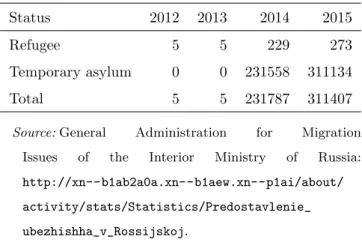
records indicate. As shown in Figure 2, the highest number of IDPs has been accommodated in eastern Ukraine. In addition to internal migration, many Ukrainians also fled to Russia, starting from 2014. Table 4 illustrates a dramatic increase in the number of Ukrainians registered with the legal status of refugee or temporary asylum in Russia which reached 311407 at the end of 2015.
Table 3: Net internal migration (persons) in the east of Ukraine over 2012-2015
Oblasts 2012 2013 2014 2015 Dnipropetrovsk -1564 -2169 431 -1177 Donetsk -4449 -4516 -10677 -9440 Kharkiv 1984 1741 8261 2739 Luhansk -4034 -4365 -8120 -5811 Zaporizhia -1361 -1916 -847 -995
Source: State Statistics Service of Ukraine: www. ukrstat.gov.ua.
In the light of these migration flows, one could on the one hand argue that migration might create attenuation bias in the main findings of our analysis, namely the negative DiD effects on political attitudes towards Russia. If pro-Ukrainian individuals left the war-affected areas to
re-29The average population in Donetsk and Luhansk oblasts is provided by the State Statistics Service of Ukraine:
www.ukrstat.gov.ua, retrieved 23 April 2016.
30
This information is published at the governmental portal: www.kmu.gov.ua/control/uk/publish/article?art_ id=248052970&cat_id=244277212, retrieved 23 April 2016. The “Ukraine Migration Profile 2014” with the numbers of IDPs for all oblasts as of 31 December 2014 is available at: www.dmsu.gov.ua/images/files/profile_2015_en. pdf, retrieved 23 April 2016.
settle somewhere else in eastern Ukraine, the drop in the support of Russia would be overesti-mated in the low treatment group (either through the migrants themselves or through interaction effects with locals) and underestimated in the high treatment group. This would squeeze the ab-solute magnitude of the negative DiD estimates. On the other hand, this could be countervailed by pro-Russian individuals leaving the war-affected area for territories outside the control of the Ukrainian government, in particular Russia. In this context, it is worth noting that the figures suggest that migration to Russia was lower than to other Ukrainian regions, such that we suspect attenuation bias to be the more relevant threat. This suggests (similarly to our identifying as-sumptions outlined below) that our main DiD effects on attitudes towards Russia are in absolute magnitude lower bounds for the true effects. Again, we notice that our estimates are not very sensitive to the choice of the socioeconomic characteristics, which one would suspect to correlate with migration decisions.
Figure 2: Internally displaced persons in thousands by destination region as of 31 March 2015
157.332 Kharkiv 154.789 Luhansk 103.758 Donetsk 82.734 Dnipropetrovsk 60.742 Zaporizhia 39.047 Kyiv City 37.060 Kyiv . . . 3.712 Volyn 3.688 Rivno 3.577 Zakarpattia 3.253 Ivano-Frankivsk 2.546 Chernivtsi 2.494 Ternopil 0 20 40 60 80 100 120 140 160
Table 4: Ukrainians registered with refugee or temporary asylum status in Russia over 2012-2015
Status 2012 2013 2014 2015
Refugee 5 5 229 273
Temporary asylum 0 0 231558 311134 Total 5 5 231787 311407
Source: General Administration for Migration Issues of the Interior Ministry of Russia: http://xn--b1ab2a0a.xn--b1aew.xn--p1ai/about/ activity/stats/Statistics/Predostavlenie_ ubezhishha_v_Rossijskoj.
5
Main results and sensitivity checks
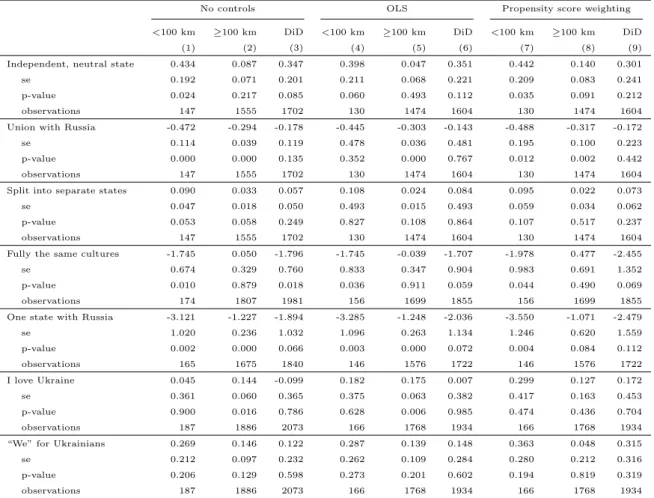
We present the results for before-after and DiD estimation based on (i) unconditional mean dif-ferences, which corresponds to setting X empty in equations (1) and (2), (ii) OLS controlling for the socioeconomic factors mentioned in Section 3, and (iii) propensity score weighting. This en-tails altogether nine different estimators. Table 5 provides the estimates for our main specification, namely when a road distance of 100 km is used to distinguish between the high and low treatment groups. Columns 1-2, 4-5, and 7-8 show the before-after estimates for the high and low treatment groups separately, whereas columns 3, 6, and 9 display the DiD estimates. Columns 1-3 contain the estimates without controls, columns 4-6 present the OLS estimates controlling for the covari-ates, and columns 7-9 report the conditional semiparametric results based on weighting.
Table 5: Estimates for a distance threshold of 100 km
No controls OLS Propensity score weighting <100 km ≥100 km DiD <100 km ≥100 km DiD <100 km ≥100 km DiD
(1) (2) (3) (4) (5) (6) (7) (8) (9) Independent, neutral state 0.434 0.087 0.347 0.398 0.047 0.351 0.442 0.140 0.301 se 0.192 0.071 0.201 0.211 0.068 0.221 0.209 0.083 0.241 p-value 0.024 0.217 0.085 0.060 0.493 0.112 0.035 0.091 0.212 observations 147 1555 1702 130 1474 1604 130 1474 1604 Union with Russia -0.472 -0.294 -0.178 -0.445 -0.303 -0.143 -0.488 -0.317 -0.172 se 0.114 0.039 0.119 0.478 0.036 0.481 0.195 0.100 0.223 p-value 0.000 0.000 0.135 0.352 0.000 0.767 0.012 0.002 0.442 observations 147 1555 1702 130 1474 1604 130 1474 1604 Split into separate states 0.090 0.033 0.057 0.108 0.024 0.084 0.095 0.022 0.073 se 0.047 0.018 0.050 0.493 0.015 0.493 0.059 0.034 0.062 p-value 0.053 0.058 0.249 0.827 0.108 0.864 0.107 0.517 0.237 observations 147 1555 1702 130 1474 1604 130 1474 1604 Fully the same cultures -1.745 0.050 -1.796 -1.745 -0.039 -1.707 -1.978 0.477 -2.455 se 0.674 0.329 0.760 0.833 0.347 0.904 0.983 0.691 1.352 p-value 0.010 0.879 0.018 0.036 0.911 0.059 0.044 0.490 0.069 observations 174 1807 1981 156 1699 1855 156 1699 1855 One state with Russia -3.121 -1.227 -1.894 -3.285 -1.248 -2.036 -3.550 -1.071 -2.479 se 1.020 0.236 1.032 1.096 0.263 1.134 1.246 0.620 1.559 p-value 0.002 0.000 0.066 0.003 0.000 0.072 0.004 0.084 0.112 observations 165 1675 1840 146 1576 1722 146 1576 1722 I love Ukraine 0.045 0.144 -0.099 0.182 0.175 0.007 0.299 0.127 0.172 se 0.361 0.060 0.365 0.375 0.063 0.382 0.417 0.163 0.453 p-value 0.900 0.016 0.786 0.628 0.006 0.985 0.474 0.436 0.704 observations 187 1886 2073 166 1768 1934 166 1768 1934 “We” for Ukrainians 0.269 0.146 0.122 0.287 0.139 0.148 0.363 0.048 0.315 se 0.212 0.097 0.232 0.262 0.109 0.284 0.280 0.212 0.316 p-value 0.206 0.129 0.598 0.273 0.201 0.602 0.194 0.819 0.319 observations 187 1886 2073 166 1768 1934 166 1768 1934
Note: Observations < 100 km to Donetsk or Luhansk form the high treatment group, while those ≥ 100 km form the low treatment group. Propensity scores are estimated by logistic regression. Standard errors are clustered on the city level using 999 bootstrap replications.
OLS and weighting deliver in general quite similar results in terms of effect magnitudes and directions. We found mostly no statistically significant shift in the sympathy towards Ukraine and self-association with Ukrainians, except for the positive and statistically significant effects based on OLS and estimation without controls regarding I love towards Ukraine in the low treatment group. In contrast, several statistically significantly negative associations were found between the proximity to the war zone and political attitudes towards Russia, which is somewhat in line with the finding of Coup´e and Obrizan (2016) that the experience of property damage decreases the support for the view that the Ukrainian government should compromise with Russia. For instance, the high treatment group’s support for the statement that Ukrainian and Russian cultures are fully the same weakened over time. While no significant change is observed in the low treatment group,
the DiD effects based on the inter-group changes in the common culture outcome over time are significantly negative at the 10% level.
Furthermore, the support for forming one common state between Ukraine and Russia signifi-cantly declined in either treatment group. The DiD estimates are also marginally significant, sug-gesting that the deterioration was larger in areas closer to the war zone. Moreover, the before-after estimates for having a preference for a political union with Russia are (with the exception of the OLS result for the high treatment group) significantly negative. In contrast, none of the corre-sponding DiD estimates is statistically significant. The share of those in the high treatment group who prefer Ukraine to remain an independent and neutral state increased significantly over time and also the DiD estimate is marginally significant for OLS and estimation without controls. In line with Coup´e and Obrizan (2016), the preference to split Ukraine into separate states appears to have increased in the high treatment group, while the DiD estimate is never significant. To sum up, both the before-after and DiD estimates suggest that the political attitudes towards Russia have deteriorated as a consequence of the war, while this is not the case for sentiments towards Ukraine. For visualization, Figure A2 in Appendix displays the frequency distributions of the non-binary outcomes in the high treatment group over time: there was a negative shift in sentiments towards Russia but no pronounced change with respect to Ukraine.
We run several sensitivity checks to investigate the robustness of our results with respect to the distance-based definition of the treatment groups. First, we examine the results when excluding Mariupol - a city located 113 km from Donetsk but nevertheless very close to the front line (see Figure 1) - from the low treatment group. Second, we vary the definition of the low treatment group as a function of distance. Specifically, we only use observations beyond 200 km from either Donetsk or Luhansk, which implies a distance window of 100 km between the high and low treatment groups that is no longer used in the analysis. Third, we base the analysis exclusively on municipalities in Donbass, to maximize cultural and geographic proximity. Fourth, we move the distance threshold for defining the high and low treatment group to 150 km which affects the composition of either group. Finally, we define the treatment not as a function of distance but based on reported military confrontations in four Donbass cities in our sample (i.e. Artemivsk, Kostiantynivka, Kramatorsk and Mariupol) to distinguish between the high and low treatment groups.
Table 6 contains the estimates when Mariupol is excluded from the low treatment group while the high treatment group and its before-after estimates remain unaffected. The estimates are
quite comparable to the previous results. For instance, we observe similar patterns in terms of sentiments towards Ukraine and Ukrainians, i.g. no significant DiD estimates. Furthermore, we find negative and mostly significant before-after and DiD estimates concerning a common state of Ukraine and Russia, negative DiD estimates on the perception of the Ukrainian and Russian cultures as fully the same, and negative before-after estimates on the preferences of both groups for a union with Russia.
Table 6: Estimates for a distance threshold of 100 km when excluding Mariupol
No controls OLS Propensity score weighting <100 km ≥100 km DiD <100 km ≥100 km DiD <100 km ≥100 km DiD
(1) (2) (3) (4) (5) (6) (7) (8) (9) Independent, neutral state 0.434 0.100 0.334 0.398 0.056 0.342 0.442 0.151 0.291 se 0.192 0.077 0.206 0.216 0.077 0.231 0.210 0.083 0.239 p-value 0.024 0.193 0.106 0.065 0.470 0.139 0.036 0.068 0.225 observations 147 1447 1594 130 1370 1500 130 1370 1500 Union with Russia -0.472 -0.300 -0.172 -0.445 -0.307 -0.138 -0.488 -0.319 -0.169 se 0.119 0.039 0.125 0.590 0.037 0.593 0.191 0.105 0.218 p-value 0.000 0.000 0.168 0.451 0.000 0.815 0.010 0.002 0.438 observations 147 1447 1594 130 1370 1500 130 1370 1500 Split into separate states 0.090 0.020 0.071 0.108 0.011 0.097 0.095 0.016 0.079 se 0.045 0.013 0.047 0.429 0.010 0.430 0.063 0.023 0.065 p-value 0.044 0.132 0.136 0.802 0.261 0.822 0.131 0.492 0.223 observations 147 1447 1594 130 1370 1500 130 1370 1500 Fully the same cultures -1.745 0.073 -1.818 -1.745 -0.001 -1.744 -1.978 0.498 -2.476 se 0.692 0.364 0.768 0.857 0.376 0.921 0.986 0.691 1.301 p-value 0.012 0.841 0.018 0.042 0.998 0.058 0.045 0.471 0.057 observations 174 1674 1848 156 1571 1727 156 1571 1727 One state with Russia -3.121 -1.211 -1.911 -3.285 -1.204 -2.081 -3.550 -1.062 -2.488 se 1.034 0.259 1.065 1.084 0.292 1.125 1.170 0.654 1.500 p-value 0.003 0.000 0.073 0.002 0.000 0.064 0.002 0.104 0.097 observations 165 1572 1737 146 1478 1624 146 1478 1624 I love Ukraine 0.045 0.155 -0.110 0.182 0.199 -0.017 0.299 0.153 0.146 se 0.358 0.067 0.363 0.382 0.064 0.386 0.420 0.163 0.439 p-value 0.899 0.020 0.762 0.634 0.002 0.965 0.477 0.348 0.740 observations 187 1750 1937 166 1637 1803 166 1637 1803 “We” for Ukrainians 0.269 0.197 0.072 0.287 0.194 0.093 0.363 0.085 0.278 se 0.206 0.088 0.230 0.251 0.106 0.270 0.275 0.223 0.314 p-value 0.192 0.026 0.755 0.252 0.067 0.730 0.187 0.703 0.375 observations 187 1750 1937 166 1637 1803 166 1637 1803
Note: Observations < 100 km to Donetsk or Luhansk form the high treatment group, while those ≥ 100 km form the low treatment group. Propensity scores are estimated by logistic regression. Standard errors are clustered on the city level using 999 bootstrap replications.
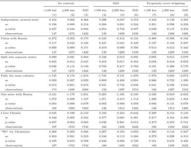
Table 7 presents the effects when reducing the low treatment group to observations more than 200 km away from Donetsk or Luhansk. The before-after estimates for the low treatment group are only marginally affected while the high treatment group is the same as in the main specification. Therefore, the DiD results are barely affected. Specifically, the DiD estimates on the similarity of
the Ukrainian and Russian cultures and on the support of a common state are again significantly negative at the 10 or 5% level, as well as the before-after estimates for a common union between Ukraine and Russia.
Table 7: Estimates when excluding cities between 100 km and 200 km
No controls OLS Propensity score weighting <100 km ≥200 km DiD <100 km ≥200 km DiD <100 km ≥200 km DiD
(1) (2) (3) (4) (5) (6) (7) (8) (9) Independent, neutral state 0.434 0.068 0.366 0.398 0.027 0.372 0.442 0.138 0.303 se 0.196 0.089 0.218 0.206 0.081 0.224 0.201 0.096 0.238 p-value 0.027 0.443 0.094 0.054 0.742 0.097 0.028 0.147 0.203 observations 147 1275 1422 130 1209 1339 130 1209 1339 Union with Russia -0.472 -0.302 -0.170 -0.445 -0.312 -0.134 -0.488 -0.306 -0.182 se 0.117 0.043 0.124 0.447 0.041 0.449 0.197 0.122 0.237 p-value 0.000 0.000 0.171 0.319 0.000 0.766 0.013 0.012 0.442 observations 147 1275 1422 130 1209 1339 130 1209 1339 Split into separate states 0.090 0.021 0.069 0.108 0.013 0.095 0.095 0.015 0.079 se 0.045 0.014 0.047 0.353 0.011 0.354 0.058 0.018 0.059 p-value 0.046 0.115 0.146 0.760 0.217 0.789 0.101 0.386 0.176 observations 147 1275 1422 130 1209 1339 130 1209 1339 Fully the same cultures -1.745 0.174 -1.919 -1.745 0.131 -1.876 -1.978 0.695 -2.672 se 0.692 0.397 0.820 0.809 0.400 0.904 0.966 0.722 1.336 p-value 0.012 0.661 0.019 0.031 0.744 0.038 0.041 0.336 0.045 observations 174 1486 1660 156 1397 1553 156 1397 1553 One state with Russia -3.121 -1.170 -1.951 -3.285 -1.185 -2.100 -3.550 -0.918 -2.633 se 1.072 0.288 1.107 1.071 0.315 1.112 1.200 0.623 1.494 p-value 0.004 0.000 0.078 0.002 0.000 0.059 0.003 0.141 0.078 observations 165 1395 1560 146 1314 1460 146 1314 1460 I love Ukraine 0.045 0.188 -0.143 0.182 0.224 -0.042 0.299 0.154 0.145 se 0.349 0.065 0.352 0.377 0.065 0.381 0.417 0.165 0.439 p-value 0.897 0.004 0.685 0.630 0.001 0.912 0.473 0.353 0.741 observations 187 1553 1740 166 1456 1622 166 1456 1622 “We” for Ukrainians 0.269 0.203 0.066 0.287 0.194 0.093 0.363 0.116 0.247 se 0.203 0.081 0.223 0.246 0.113 0.266 0.272 0.228 0.313 p-value 0.185 0.013 0.768 0.242 0.086 0.726 0.181 0.610 0.430 observations 187 1553 1740 166 1456 1622 166 1456 1622
Note: Observations < 100 km to Donetsk or Luhansk form the high treatment group, while those ≥ 200 km form the low treatment group. Propensity scores are estimated by logistic regression. Standard errors are clustered on the city level using 999 bootstrap replications.
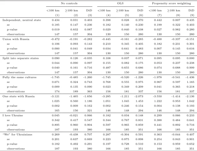
In Table 8, we report the estimates for the Donbass subsample with at most 193 observations in the high treatment group versus 187 observations in the low treatment group, given the distance threshold of 100 km as in the main specification. This sensitivity check is motivated by the potential concern that Donbass is, despite many historical and cultural similarities with the remainder of the east, nevertheless distinct from other regions in a way that makes the common trend assumption fail when relying on the observations outside of Donbass. Statistical power is now considerably
statistically significant at the 10% level. It is nevertheless reassuring that the magnitudes are qualitatively in line with the previous key findings. They again suggest that the preferences for political ties with Russia have weakened.
Table 8: Estimates for Donbass only with a distance threshold of 100 km
No controls OLS Propensity score weighting <100 km ≥100 km DiD <100 km ≥100 km DiD <100 km ≥100 km DiD
(1) (2) (3) (4) (5) (6) (7) (8) (9) Independent, neutral state 0.434 0.031 0.403 0.398 0.028 0.370 0.442 0.007 0.435 se 0.185 0.147 0.236 0.182 0.140 0.230 0.199 0.322 0.403 p-value 0.019 0.832 0.087 0.029 0.840 0.108 0.027 0.982 0.280 observations 147 157 304 130 150 280 130 150 280 Union with Russia -0.472 -0.191 -0.282 -0.445 -0.161 -0.285 -0.488 -0.337 -0.151 se 0.106 0.093 0.143 0.210 0.345 0.405 0.182 0.231 0.301 p-value 0.000 0.041 0.049 0.034 0.641 0.483 0.007 0.145 0.616 observations 147 157 304 130 150 280 130 150 280 Split into separate states 0.090 0.126 -0.035 0.108 0.037 0.071 0.095 0.095 0.000 se 0.044 0.090 0.097 0.155 0.082 0.175 0.053 0.237 0.238 p-value 0.040 0.161 0.716 0.487 0.655 0.686 0.074 0.688 0.999 observations 147 157 304 130 150 280 130 150 280 Fully the same cultures -1.745 -0.485 -1.260 -1.745 -0.520 -1.226 -1.978 -0.541 -1.436 se 0.671 0.324 0.743 0.768 0.555 0.975 0.967 0.597 1.165 p-value 0.009 0.135 0.090 0.023 0.349 0.209 0.041 0.365 0.218 observations 174 189 363 156 181 337 156 181 337 One state with Russia -3.121 -1.465 -1.656 -3.285 -1.211 -2.073 -3.550 -1.414 -2.136 se 1.025 0.560 1.186 1.051 1.045 1.453 1.222 0.953 1.642 p-value 0.002 0.009 0.162 0.002 0.246 0.154 0.004 0.138 0.193 observations 165 156 321 146 148 294 146 148 294 I love Ukraine 0.045 -0.021 0.066 0.182 0.034 0.148 0.299 0.066 0.233 se 0.342 0.417 0.547 0.344 0.767 0.831 0.388 0.484 0.641 p-value 0.895 0.960 0.904 0.597 0.965 0.859 0.441 0.892 0.716 observations 187 193 380 166 185 351 166 185 351 “We” for Ukrainians 0.269 -0.438 0.707 0.287 -0.304 0.591 0.363 -0.044 0.407 se 0.201 0.637 0.669 0.223 0.875 0.898 0.254 0.843 0.901 p-value 0.182 0.492 0.291 0.197 0.728 0.510 0.153 0.959 0.652 observations 187 193 380 166 185 351 166 185 351
Note: Observations < 100 km to Donetsk or Luhansk form the high treatment group, while those ≥ 100 km form the low treatment group. Propensity scores are estimated by logistic regression. Standard errors are clustered on the city level using 999 bootstrap replications.
Next, we shift the distance threshold further away from the front zone. Thus, the high treatment group expands to seven municipalities in Donbass while the low treatment group is now reduced accordingly. Table 9 provides the results. For most variables, the magnitudes of the before-after estimates in the high treatment group decrease while the sizes of those for the low treatment group increase compared to Table 5. Therefore, this specification generally yields smaller and less statistically significant DiD estimates than the main specification, but nevertheless qualitatively
similar. The negative before-after estimates for a union, as well as for forming one state with Russia remain statistically significant for either treatment group. In the high treatment group, the before-after estimates for belonging to the same culture are borderline significant. The negative DiD estimates for belonging to the same culture are also marginally significant in two out of three cases, while the ones on forming one state are not any more.
Table 9: Estimates for a distance threshold of 150 km
No controls OLS Propensity score weighting <150 km ≥150 km DiD <150 km ≥150 km DiD <150 km ≥150 km DiD
(1) (2) (3) (4) (5) (6) (7) (8) (9) Independent, neutral state 0.218 0.093 0.126 0.259 0.048 0.211 0.308 0.163 0.144 se 0.178 0.076 0.193 0.163 0.077 0.181 0.159 0.084 0.174 p-value 0.219 0.221 0.515 0.113 0.530 0.243 0.053 0.052 0.406 observations 281 1421 1702 258 1346 1604 258 1346 1604 Union with Russia -0.358 -0.306 -0.052 -0.358 -0.311 -0.046 -0.402 -0.357 -0.045 se 0.102 0.040 0.109 0.117 0.039 0.122 0.159 0.074 0.179 p-value 0.000 0.000 0.633 0.002 0.000 0.703 0.012 0.000 0.800 observations 281 1421 1702 258 1346 1604 258 1346 1604 Split into separate states 0.128 0.022 0.106 0.116 0.013 0.103 0.103 0.017 0.086 se 0.049 0.012 0.051 0.250 0.010 0.250 0.062 0.015 0.064 p-value 0.009 0.084 0.037 0.643 0.210 0.680 0.097 0.251 0.181 observations 281 1421 1702 258 1346 1604 258 1346 1604 Fully the same cultures -1.183 0.094 -1.278 -1.109 0.027 -1.136 -1.054 0.159 -1.213 se 0.565 0.361 0.672 0.584 0.380 0.698 0.669 0.533 0.976 p-value 0.036 0.794 0.057 0.057 0.943 0.104 0.115 0.766 0.214 observations 335 1646 1981 310 1545 1855 310 1545 1855 One state with Russia -2.363 -1.229 -1.134 -2.489 -1.214 -1.275 -2.463 -1.178 -1.284 se 0.796 0.260 0.823 0.876 0.285 0.926 0.992 0.493 1.214 p-value 0.003 0.000 0.168 0.005 0.000 0.168 0.013 0.017 0.290 observations 295 1545 1840 269 1453 1722 269 1453 1722 I love Ukraine -0.018 0.177 -0.195 0.088 0.216 -0.128 0.074 0.143 -0.069 se 0.264 0.059 0.271 0.255 0.061 0.263 0.268 0.123 0.314 p-value 0.945 0.003 0.471 0.729 0.000 0.627 0.782 0.245 0.827 observations 352 1721 2073 324 1610 1934 324 1610 1934 “We” for Ukrainians -0.243 0.235 -0.478 -0.141 0.223 -0.364 -0.185 0.128 -0.313 se 0.299 0.088 0.310 0.249 0.112 0.272 0.293 0.199 0.348 p-value 0.416 0.007 0.124 0.570 0.046 0.180 0.527 0.521 0.369 observations 352 1721 2073 324 1610 1934 324 1610 1934
Note: Observations < 150 km to Donetsk or Luhansk form the high treatment group, while those ≥ 150 km form the low treatment group. Propensity scores are estimated by logistic regression. Standard errors are clustered on the city level using 999 bootstrap replications.
For four of the cities in the Donetsk oblast that are included in our sample, we found that they directly experienced military confrontations in 2014 based on Internet research and checks of the movement of the front according to the maps of the Information Analysis Center of the National Security and Defense Council of Ukraine. In a further robustness check, we assign these cities to
the high treatment group, while all remaining cities in our sample form the low treatment group. The cities in the newly defined high treatment group are located close to the front line, i.e. less than 100 km to Donetsk or Luhansk except for Mariupol. Therefore, the results in Table 10 are mostly in line with the results of the main specification, albeit generally less significant. In partic-ular, while the negative OLS based-DiD effects on the common culture and one state outcomes are borderline significant, the weighting-based estimates are quite imprecise, albeit similar in magni-tude. We conclude that our battery of robustness checks by and large confirms the findings of the main specification, namely that the political capital of Russia decreased in the government-held territories in eastern Ukraine affected by the war, while mostly no statistically significant effects are found with respect to sentiments towards Ukraine.
Table 10: Estimates for military confrontations
No controls OLS Propensity score weighting battle no battle DiD battle no battle DiD battle no battle DiD
(1) (2) (3) (4) (5) (6) (7) (8) (9) Independent, neutral state 0.105 0.116 -0.011 0.155 0.075 0.080 0.209 0.165 0.045 se 0.241 0.074 0.253 0.309 0.076 0.321 0.218 0.108 0.252 p-value 0.663 0.115 0.964 0.616 0.323 0.804 0.337 0.126 0.859 observations 207 1495 1702 194 1410 1604 194 1410 1604 Union with Russia -0.426 -0.300 -0.126 -0.476 -0.307 -0.168 -0.582 -0.365 -0.217 se 0.146 0.039 0.151 1.000 0.037 1.000 0.212 0.121 0.271 p-value 0.004 0.000 0.403 0.634 0.000 0.866 0.006 0.003 0.423 observations 207 1495 1702 194 1410 1604 194 1410 1604 Split into separate states 0.167 0.021 0.146 0.168 0.012 0.155 0.144 0.008 0.136 se 0.047 0.012 0.048 0.750 0.010 0.750 0.1 0.028 0.101 p-value 0.000 0.090 0.002 0.823 0.214 0.836 0.15 0.762 0.179 observations 207 1495 1702 194 1410 1604 194 1410 1604 Fully the same cultures -1.299 0.049 -1.348 -1.380 -0.021 -1.359 -1.166 0.078 -1.244 se 0.784 0.347 0.862 0.749 0.364 0.833 0.842 0.725 1.338 p-value 0.097 0.889 0.118 0.065 0.954 0.103 0.166 0.914 0.352 observations 256 1725 1981 239 1616 1855 239 1616 1855 One state with Russia -3.094 -1.189 -1.905 -3.161 -1.205 -1.956 -3.18 -1.121 -2.059 se 0.913 0.246 0.933 1.053 0.277 1.098 1.208 0.715 1.555 p-value 0.001 0.000 0.041 0.003 0.000 0.075 0.008 0.117 0.186 observations 217 1623 1840 200 1522 1722 200 1522 1722 I love Ukraine 0.078 0.161 -0.083 0.088 0.211 -0.123 0.081 0.123 -0.042 se 0.353 0.064 0.357 0.437 0.063 0.441 0.426 0.175 0.438 p-value 0.824 0.012 0.817 0.841 0.001 0.780 0.849 0.483 0.924 observations 270 1803 2073 252 1682 1934 252 1682 1934 “We” for Ukrainians -0.139 0.200 -0.338 -0.091 0.204 -0.295 -0.156 0.015 -0.171 se 0.312 0.088 0.325 0.310 0.107 0.328 0.294 0.206 0.349 p-value 0.657 0.024 0.298 0.769 0.057 0.368 0.595 0.943 0.625 observations 270 1803 2073 252 1682 1934 252 1682 1934
Note: Military confrontations in 2014 were reported for Artemivsk, Kostiantynivka, Kramatorsk and Mariupol. Propensity scores are estimated by logistic regression. Standard errors are clustered on the city level using 999 bootstrap replications.
To investigate effect heterogeneity across language, Table A5 in the Appendix presents our main analysis for the subsample of native Russian speakers, who could differ in attitudes and effects from native Ukrainian speakers. However, the results are qualitatively similar to those in the total sample. Furthermore, we examine effect heterogeneity across age groups by considering the subsample below the median age of 45 in the evaluation sample. Table A6 in Appendix displays the obtained results that are in line with those in the whole sample. As a final check, we examined whether item non-response in the outcome variables is selective in our sample, i.e. varies systematically over time and across treatment groups. For this purpose, we created missing dummies for our outcomes of interest and used them as dependent variables in our estimators. We generally found no evidence for selective item non-response within treatment groups over time or across time trends of treatment groups (see Table A7 in Appendix).
6
Placebo tests
To complement the sensitivity checks, we conduct two placebo tests for our DiD approach in which we assign treatment based on distance to a certain municipality in a region relatively far from the war zone such that war exposure should be perceived as equally low in the entire region. A further criterion is that the region should be culturally rather homogeneous and should not ex-perience a large inflow of IDPs from the war zone (see Figure 2). For these reasons, we picked two regions in the north and the west center of Ukraine (see Figure 3). Following the historically motivated definitions in Denisova-Schmidt and Huber (2014), the northern region includes Cherni-hiv, Sumy, Poltava, Cherkasy, and Kirovohrad oblasts; the west central region consists of Volyn, Rivno, Zhytomyr, Khmelnytsk, and Vinnytsia oblasts. Within each region, the placebo groups with the high and low treatment are defined based on the road distance (by car) to a particular city chosen to meet two criteria: first, it is not one of Ukrainian major cities in terms of political or military power; second, the resulting placebo groups include a sufficient number of observations to implement the DiD approach. For the north of Ukraine, we consider the distance to Oleksandria (Kirovohrad oblast); for the west center, we take the distance to Zhytomyr (Zhytomyr oblast). Only the cities observed in both survey waves enter our sample, i.e. 18 cities in the west center region and 14 cities in the north.
We compare observations within a 100 km radius from the respective target city to those further away in each region and apply the same three DiD approaches as used in the previous section.