HAL Id: inria-00164599
https://hal.inria.fr/inria-00164599v2
Submitted on 23 Jul 2007
HAL is a multi-disciplinary open access
archive for the deposit and dissemination of
sci-entific research documents, whether they are
pub-lished or not. The documents may come from
teaching and research institutions in France or
abroad, or from public or private research centers.
L’archive ouverte pluridisciplinaire HAL, est
destinée au dépôt et à la diffusion de documents
scientifiques de niveau recherche, publiés ou non,
émanant des établissements d’enseignement et de
recherche français ou étrangers, des laboratoires
publics ou privés.
Performance Evaluation of Scheduling Policies for
Volunteer Computing
Derrick Kondo, David Anderson, John Mcleod Vii
To cite this version:
Derrick Kondo, David Anderson, John Mcleod Vii. Performance Evaluation of Scheduling Policies for
Volunteer Computing. [Technical Report] 2007. �inria-00164599v2�
Performance Evaluation of Scheduling Policies for Volunteer Computing
Derrick Kondo
1David P. Anderson
2John McLeod VII
3 1INRIA, France
2University of California at Berkeley, U.S.A.
3Sybase Inc., U.S.A.
Abstract
BOINC, a middleware system for volunteer computing, al-lows hosts to be attached to multiple projects. Each host periodically requests jobs from project servers and executes the jobs. This process involves three interrelated policies: 1) of the runnable jobs on a host, which to execute? 2) when and from what project should a host request more work? 3) what jobs should a server send in response to a given re-quest? 4) How to estimate the remaining runtime of a job? In this paper, we consider several alternatives for each of these policies. Using simulation, we study various combi-nations of policies, comparing them on the basis of several performance metrics and over a range of parameters such as job length variability, deadline slack, and number of at-tached projects.
1
Introduction
Volunteer computing is a form of distributed comput-ing in which the general public volunteers processcomput-ing and storage resources to computing projects. Early volunteer computing projects include the Great Internet Mersenne Prime Search [12] and Distributed.net [1]. BOINC (Berke-ley Open Infrastructure for Network Computing) is a mid-dleware system for volunteer computing [6, 3]. BOINC projects are independent; each has its own server, applica-tions, and jobs. Volunteers participate by running BOINC client software on their computers (hosts). Volunteers can attach each host to any set of projects. There are currently about 40 BOINC-based projects and about 400,000 vol-unteer computers performing an average of over 500 Ter-aFLOPS.
BOINC software consists of client and server compo-nents. The BOINC client runs projects’ applications, and performs CPU scheduling (implemented on top of the lo-cal operating system’s scheduler). All network communi-cation in BOINC is initiated by the client; it periodically requests jobs from the servers of projects to which it is attached. Some hosts have intermittent physical network connections (for example, portable computers or those with modem connections). Such computers may connect only
every few days, and BOINC attempts to download enough work to keep the computer busy until the next connection.
This process of getting and executing jobs involves four interrelated policies:
1. CPU scheduling: of the currently runnable jobs, which to run?
2. Work fetch: when to ask a project for more work, which project to ask, and how much work to ask for? 3. Work send: when a project receives a work request,
which jobs should it send?
4. Completion time estimation: how to estimate the re-maining CPU time of a job?
These policies have a large impact on the performance of BOINC-based projects. Because studying these policies in situ is difficult, we have developed a simulator that mod-els a BOINC client and a set of projects. We have used this simulator to compare several combinations of schedul-ing policies, over a range of parameters such as job-length variability, deadline slack, and number of attached projects. With the simulator, our main goals are to show the effec-tiveness of scheduling policies in scenarios representative of current project workloads, and also hypothetical extreme scenarios that reflect the scheduler’s ability to deal with new future job workloads.
The remainder of the paper is organized as follows. In Section 2, we describe various scheduling policies in de-tail. Then in Section 3, we detail the simulator and its input parameters. In Section 4, we describe our metrics for eval-uating the different aspects of each scheduling policy. In Sections 5 and 6, we present the results of our evaluation and deployment. In Section 7, we compare and contrast our work with other related work. Finally, in Section 8, we summarize the main conclusions of this paper, and describe directions for future work.
2
Scheduling Policy Details
The scheduling policies have several inputs. First, there are the host’s hardware characteristics, such as number of processors and benchmarks. The client tracks various usage
characteristics, such as the active fraction (the fraction of time BOINC is running and is allowed to do computation), and the statistics of its network connectivity.
Second, there are user preferences. These include: • A resource share for each project.
• Limits on processor usage: whether to compute while the computer is in use, the maximum number of CPUs to use, and the maximum fraction of CPU time to use (to allow users to reduce CPU heat).
• ConnectionInterval: the minimum time between peri-ods of network activity. This lets users provide a ”hint” about how often they connect, and it lets modem users tell BOINC how often they want it to automatically connect.
• SchedulingInterval: the ”time slice” of the BOINC client CPU scheduler (the default is one hour). • WorkBufMinDays: how much work to buffer.
• WorkBufAdditional: how much work to buffer beyond WorkBufMinDays.
Finally, each job (that is, unit of work) has a num-ber of project-specified parameters, including estimates of its number of floating-point operations, and a deadline by which it should be reported. Most BOINC projects use replicated computing, in which two or more instances of each job are processed on different hosts. If a host doesn’t return a job by its deadline, the user is unlikely to receive credit for the job. We will study two or three variants of each policy, as described below.
2.1
CPU Scheduling Policies
CS1: round-robin time-slicing between projects, weighted according to their resource share.
CS2: do a simulation of weighted round-robin (RR)
scheduling, identifying jobs that will miss their deadlines. Schedule such jobs earliest deadline first (EDF). If there are remaining CPUs, schedule other jobs using weighted round-robin.
2.2
Work fetch policies
WF1: keep enough work queued to last for
WorkBuf-MinDays+WorkBufAdditional, and divide this queue be-tween projects based on resource share, with each project always having at least one job running or queued.
WF2: maintain the ”long-term debt” of work owed to
each project. Use simulation of weighted round-robin to es-timate its CPU shortfall. Fetch work from the project for
which debt - shortfall is greatest. Avoid fetching work re-peatedly from projects with tight deadlines. The details of this policy are given in [16].
2.3
Work Send Policies
WS1: given a request for X seconds of work, send a
set of jobs whose estimated run times (based on FLOPS estimates, benchmarks, etc.) are at least X.
WS2: the request message includes a list of all jobs in
progress on the host, including their deadlines and comple-tion times. For each ”candidate” job J, do an EDF simula-tion of the current workload with J added. Send J only if it meets its deadline, all jobs that currently meet their dead-lines continue to do so, and all jobs that miss their deaddead-lines don’t miss them by more.
2.4
Job Completion Estimation Policies
JC1: BOINC applications report their fraction done
pe-riodically during execution. The reliability of an estimate based on fraction done presumably increases as the job pro-gresses. Hence, for jobs in progress BOINC uses the esti-mate F A+ (1 − F )B where F is the fraction done, A is
the estimate based on elapsed CPU time and fraction done, and B is the estimate based on benchmarks, floating-point count, user preferences, and CPU efficiency (the average ratio of CPU time to wall time for this project).
JC2: maintain a per-project duration correction factor
(DCF), an estimate of the ratio of actual CPU time to originally estimated CPU time. This is calculated in a conservative way; increases are reflected immediately, but decreases are exponentially smoothed.
An “overall” policy is a choice of each sub-policy (for example, CS2 WF2 WS2 JC2).
3
Scheduling Scenarios
We evaluate these scheduling policies using a simula-tor of the BOINC client. The simulasimula-tor simulates the CPU scheduling logic and work-fetch policies of the client ex-actly down to the source code itself. This was made possible by refactoring the BOINC client source code such that the scheduler code is cleanly separated from the code required for networking and memory access. As such, the simulator links to the real BOINC scheduling code with little modi-fication. In fact, only the code for network accesses (i.e., RPC’s to communicate with the project and data servers) are substituted by simulation stubs. Thus, the scheduling logic and almost all the source code of the simulated client are identical to the real one.
Parameter Value
duration 100 days delta 60 seconds
Table 1. Simulator Parameters.
Parameter Value
resource share 100 latency bound 9 days job FPOPS estimate 1.3e13 (3.67
hours on a dedicated 3GHz host) job FPOPS mean 1.3e13 (3.67
hours) FPOPS std dev 0
Table 2. Project Parameters.
The simulator allows specification of the following pa-rameters:
• For a host:
– Number of CPUs and CPU speed. – Fraction of time available
– Length of availability intervals as an exponential
distribution with parameter λavail
– ConnectionInterval
• For a client:
– CPU scheduling interval
– WorkBufMinDays, WorkBufAdditional
• For each project:
– Resource share
– Latency bound (i.e., a job deadline) – Job FLOPs estimate
– Job FLOPs actual distribution (normal)
Each combination of parameters is called a scenario. When conducting the simulation experiments, we use the values shown in Tables 1,2,3, and 4 as the base input pa-rameters to the simulator. In our simulation experiments, we vary one or a small subset of these parameter settings as we keep the other parameter values constant. This is useful for identifying the (extreme) situations where a particular scheduling policy performs poorly.
Parameter Value
number of cpus 2 dedicated cpu speed in FPOPS 1e9
fraction of time available 0.8
λavail 1,000
ConnectionInterval 0
Table 3. Host Parameters.
Parameter Value
CPU scheduling period 60 minutes WorkBufMinDays 0.1 days (2.4
hours) ) WorkBufAdditional 0.25 days (6
hours)
Table 4. Client Parameters.
The values shown in these tables are chosen to be as re-alistic as possible using data collected from real projects, as the accuracy of the simulation depends heavily on these values and their proportions relative to one another. For the host and project parameters, we use the median values found from real BOINC projects as described in [7, 2]. For the client parameters, we use the default values in the real client. More details about the selection of these values can be found in the Appendix.
4
Performance metrics
We use the following metrics in evaluating scheduling policies:
1. Idleness: of the total available CPU time, the fraction that is unused because there are no runnable jobs. This is in [0,1], and is ideally zero.
2. Waste: of the CPU time that is used, the fraction used by jobs that miss their deadline.
3. Share violation: a measure of how closely the user’s resource shares are respected, where 0 is best and 1 is worst.
4. Monotony: an inverse measure of how often the host switches between projects: 0 is as often as possible (given the scheduling interval and other factors) and 1 means there is no switching. This metric represents the fact that if a volunteer has devoted equal resource share to two projects, and sees his computer running only one of them for a long period, he will be dissatisfied.
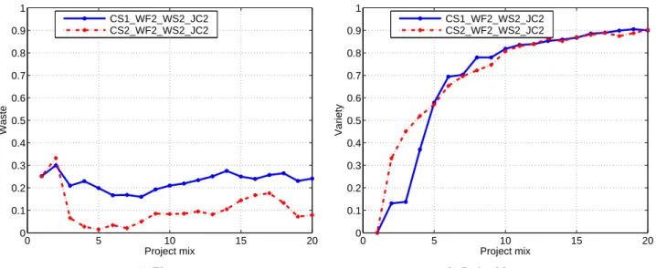
0 5 10 15 20 0 0.1 0.2 0.3 0.4 0.5 0.6 0.7 0.8 0.9 1 Project mix Waste CS1_WF2_WS2_JC2 CS2_WF2_WS2_JC2 (a) Waste 0 5 10 15 20 0 0.1 0.2 0.3 0.4 0.5 0.6 0.7 0.8 0.9 1 Project mix Variety CS1_WF2_WS2_JC2 CS2_WF2_WS2_JC2 (b) Project Monotony
Figure 1. CPU Scheduling
5
Results and Discussion
5.1
CPU scheduling policies
In this section, we compare a policy that only uses round-robin time-slicing (CS1 WF2 WS2 JC2) with a policy that will potentially schedule (some) tasks in EDF fashion if their deadlines are at risk of being missed (CS2 WF2 WS2 JC2).
To simulate a real workload of projects, we must ensure that there are a mix of projects with a variety of job sizes and deadlines. So, we define the term mix as follows. A work-load has mix M if it contains M projects, and the client is registered with each project Piwhere1 ≤ i ≤ M , and each
project Pihas the following characteristics:
1. mean FPOPS per job = i × FPOPS base 2. latency bound = i × latency bound base 3. resource share = i × resource share base
where the base values are those values defined in Ta-bles 1, 3, and 4.
We vary M from 1 to 20 for each simulation workload. The results are shown in Figure 1. We observe that CS2 WF2 WS2 JC2 often outperforms CS1 WF2 WS2 JC2 by more than 10% in terms of waste for when the project mix is greater than 3. The improved performance of CS2 WF2 WS2 JC2 can be explained by the switch to EDF mode when job deadlines are in jeop-ardy.
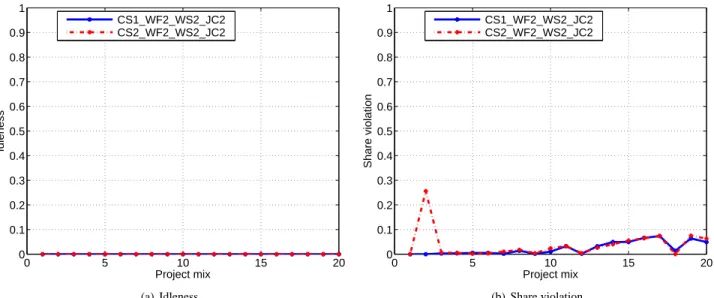
In terms of share idleness, share violation, and project monotony, the performance of CS2 WF2 WS2 JC2 and
CS1 WF2 WS2 JC2 are roughly equivalent. Share viola-tion is low, usually below 0.10, and increases only slightly with the number projects and mix (see Figure 7 in Ap-pendix). With respect to idleness, both policies have remarkably low (near zero) idleness for any number of projects and mix (see Figure 7 in Appendix). By con-trast, project monotony tends to increase greatly with the project mix. We find that relatively long jobs can often cause monotony, particularly when the job is at risk of miss-ing a deadline and the scheduler switches to EDF mode to help ensure its timely completion. Indeed, an increase in monotony with job length is inevitable but acceptable, given the more important goal of meeting job deadlines and to minimize waste. Thus, in almost all cases, the policy CS2 WF2 WS2 JC2 combining EDF with RR outperforms or performs as well as CS1 WF2 WS2 JC2.
As a side effect of these experiments, we determine the scalability of the BOINC client with respect to the num-ber of projects. (One could ask how a user could register with 20 projects. This scenario could very well arise as the number of projects is rapidly increasing, and the idea of project “mutual funds” has been proposed, where projects are group together by certain characteristics [for example, non-profit, computational biology], and users register for funds instead of only projects.)
We find that even when the number of projects is high at 20, waste, idleness, and share violation remain relatively constant throughout the range between 1-20. The exception is with project monotony which increases rapidly but is ac-ceptable. Thus, we conclude the scheduler scales with the number of projects. For the remainder of this subsection, we investigate further the CS2 WF2 WS2 JC2 policy with
respect to deadline slack and buffer size. 5.1.1 Deadline slack 0 10 20 30 40 50 60 0 0.1 0.2 0.3 0.4 0.5 0.6 0.7 0.8 0.9 1 Slack
Waste, idleness, or share violation
0 10 20 30 40 50 600 0.1 0.2 0.3 0.4 0.5 0.6 0.7 0.8 0.9 1 Monotony waste idleness share violation monotony Figure 2. Slack
In this section, we investigate the sensitivity of CS2 WF2 WS2 JC2 to the latency bound relative to the mean job execution time on a dedicated machine. We de-fine the slack to be the ratio of the latency bound to the mean FPOPS estimate multiplied by the inverse of the host speed.
We then run simulations testing the scheduler with sin-gle project and a range of slack values from 1 to 60. A slack of 1 means that the latency bound is roughly equivalent to execution time. A slack of 60 means that the latency bound is 60 times greater than the mean execution time on a dedi-cated machine. We select this maximum value because it in fact represents the median slack among all existing BOINC projects [7]. That is, the execution of jobs in many projects is on the order of hours, where as the latency bound is in terms of days.
Figure 2 shows the result of the simulation runs testing slack. Obviously, the share violation and monotony are 0 since we only have a single project. The idleness is 0 be-cause of the low connection interval and so the scheduler does a perfect job of requesting work. However, it tends to fetch more than it can compute. We find that for a slack of 1, waste is 1, and quickly drops to 0 when slack reaches 5. The waste corresponding to slack values of 2, 3, 4, and 5 are 0.75, 0.24, 0.02, and 0 respectively. Thereafter, for slack values greater than or equal to 5, waste remains at 0. After careful inspection of our simulation experiments, we find that the unavailability of the host (set to be 20% of the time) is one main factor that causes the high waste value when the slack is near 1. That is, if a host is unavailable 20% of the time, then a 3.67-hour job on a dedicated machine will
take about 4.58 hours on average and likely surpass the 3.67 hour latency bound.
Another cause of the waste is the total work buffer size, which is set at a default of 0.35 (= 0.25 + 0.1) days. When
the work buffer size is specified, the client ensures that it re-trieves at least that amount of work with each request. Set-ting a value that is too high can result in retrieving too much work that cannot be completed in time by the deadline. We investigate this issue further the following section.
5.1.2 Buffer size
To support our hypothesis that the buffer size is a major fac-tor that contributes to waste, we ran simulations with differ-ent buffer sizes. In particular, we determined how waste varies as function of the buffer size and slack. We varied slack for from 1 to 5, which corresponded to the range of slack values in Figure 2 that resulted positive waste (except when slack was 5, where the waste was 0). We varied the buffer size between about 1 to 8.4 hours of work. The max-imum value in that range corresponds to the default buffer size used by the client, i.e. 0.35 days, and used for the ex-periments with slack in Section 5.1.1.
1 2 3 4 5 1 3 5 7 9 0 0.2 0.4 0.6 0.8 1
Tot buf (hours) Slack
Waste
Figure 3. Waste as a function of minimum buffer size and slack
Figure 3 shows the result of our simulation runs. The differences in color of each line segment correspond to a different value of waste. When the buffer size is at its max-imum value, the resulting waste as a function of slack is identical to the waste seen in Figure 2. As the buffer size is lowered, the waste (and number of deadlines missed) dra-matically decreases. For the case where slack is 2, waste is constant for buffer sizes between 5 to 7 hours. The rea-son this occurs is simply because of job sizes are about 3.67
0 5 10 15 20 0 0.1 0.2 0.3 0.4 0.5 0.6 0.7 0.8 0.9 1 Project mix Waste CS2_WF1_WS2_JC2 CS2_WF2_WS2_JC2 (a) Waste 0 5 10 15 20 0 0.1 0.2 0.3 0.4 0.5 0.6 0.7 0.8 0.9 1 Project mix Share violation CS2_WF1_WS2_JC2 CS2_WF2_WS2_JC2 (b) Share violation
Figure 4. Work fetch
hours in length, and so incremental increases in the buffer size may not change the number of jobs downloaded from the server.
While decreasing the buffer size can also decrease waste, the exception is when the slack is 1; waste remains at 1 re-gardless of the buffer size. This is due to the host unavail-ability and its effect on job execution time. It has a lesser effect when slack reaches 2 since the host is unavailable only 20% of the time, and corresponds to a slowdown less than 2.
We conclude that decreasing the work buffer size can re-sult in tremendous reduction in waste, but the benefits are limited by the availability of the client. However, one can-not set the work buffer size arbitrarily low since it could result in frequent flooding of the server with work requests from clients. We will investigate this interesting issue in future work.
5.2
Work Fetch Policies
In this section, we compare two ways of determining which project to ask for more work, and how much work to ask for. When forming a work request, the first policy (CS2 WF1 WS2 JC2) tries to ensure that the work queue is filled by asking for work based on the resource shares so that at least one job is running or queued. The second policy (CS2 WF2 WS2 JC2) determines how much “long-term debt” is owed to each project, and fetches work from the project with the largest difference between the debt and shortfall. (Details of each policy can be found in [16]).)
We find that waste for CS2 WF1 WS2 JC2 tends to in-crease dramatically with the project mix (see Figure 4(a)),
and that the share violation is relatively high (see Fig-ure 4(b)) as jobs for projects with tight deadlines are down-loaded, and preempt other less urgent jobs, causing them to miss their deadlines. By contrast, CS2 WF2 WS2 JC2 im-proves waste by as much as 90% and share violation by as much as 50% because the policy avoids fetching work from projects with tight deadlines. (Idleness and monotony for the two policies were almost identical.)
5.3
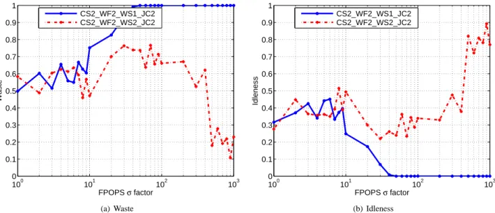
Work Send Policies
In this section we compare two policies for sending work from the server. The first policy (CS2 WF2 WS1 JC2) simply sends the amount of work requested by the client. The second policy (CS2 WF2 WS2 JC2) checks via server-side online EDF simulation if the newly re-quested jobs would meet their deadlines, if all jobs in progress on the client would continue to meet their dead-lines, and if all jobs in progress on the client that miss their deadlines don’t miss them by more.
We found that the second work send policy CS2 WF2 WS2 JC2 is advantageous only when there are relatively many jobs on the client (having a large work queue buffer), and if the amount of work per job has high variance. This would create the “ideal” situation where new jobs could disrupt jobs in-progress. So to show the effectiveness of work send policies, we increased the connection interval and work buffer size to 2 days, varied the standard deviation of the FPOPS per job by a factor of
s relative to the mean job size, and created two projects
with equal resources shares and job sizes that differed by a factor of 10.
100 101 102 103 0 0.1 0.2 0.3 0.4 0.5 0.6 0.7 0.8 0.9 1 FPOPS σ factor Waste CS2_WF2_WS1_JC2 CS2_WF2_WS2_JC2 (a) Waste 100 101 102 103 0 0.1 0.2 0.3 0.4 0.5 0.6 0.7 0.8 0.9 1 FPOPS σ factor Idleness CS2_WF2_WS1_JC2 CS2_WF2_WS2_JC2 (b) Idleness
Figure 5. Work send
In Figure 5, we vary the standard deviation of the job size by a factor s between 1 to 1000. We find that CS2 WF2 WS2 JC2 often outperforms CS2 WF2 WS1 JC2 by 20% or more in terms of waste, at the cost of idleness, which is often higher by 20% or more. The main reason for this result is that CS2 WF2 WS2 JC2 is naturally more conservative in sending job to clients, which reduces deadline misses but in turn causes more fre-quent idleness.
5.4
Job Completion Estimation Policies
1 2 3 4 5 6 7 8 9 10 0 0.1 0.2 0.3 0.4 0.5 0.6 0.7 0.8 0.9 1
Work estimate error factor
Waste
CS2_WF2_WS2_JC1 CS2_WF2_WS2_JC2
Figure 6. Job Completion
To create a project and when forming jobs, the
appli-cation developer must provide an estimate of the amount of work in FPOPS per job. This estimate in turn is used by the client scheduler along with the job deadline to form work requests and to determine which job to schedule next. However, user estimates are often notoriously off from the actual amount of work. This has been evident in both vol-unteer computing systems such as BOINC and also with the usage of traditional MPP’s [14]. As such, the scheduler uses a duration correction factor to offset any error in estimation based on the history of executed jobs.
In this section, we measure the impact of using DCF for a range of estimation errors by comparing
CS1 WF2 WS2 JC1 with CS1 WF2 WS2 JC2.
Let f be the error factor such that the user estimated work per job is given by the actual work divided by f . When
f = 1, the user estimate matches the actual precisely. When f > 1, then the user estimate under-estimates the amount
of real work.
We observe that initially when the estimate matches the actual, then both policies with DCF (when it is adjusted to offset any error) and without DCF (when it is always set to 1) have identical performance in terms of waste (see Fig-ure 6). For higher error factors, the policy with DCF greatly outperforms the policy that omits it. The waste for DCF remains remarkably constant regardless of the error factor while the waste for the non-DCF policies shoots up quickly. In fact, the waste reaches nearly 1 when the work estimate is 4 times less than the actual. With respect to the speed of convergence to the correct DCF, we found that the DCF converges immediately to the correct value after the ini-tial work fetch, after inspecting our simulation traces. (For conciseness, note that we only show the figure for waste;
all other values for idleness, share violation, and project monotony were zero.)
6
Deployment
The client scheduler has been implemented in C++ and deployment across about one million hosts over the Inter-net [6, 3]. One of the primary metrics for performance in the real-world settings is feedback from users about the scheduling policies. Users have a number of ways of di-rectly or indidi-rectly monitoring the client scheduling, includ-ing the ability to log the activities of the client scheduler with a simple debug flag, or the amount of credit granted to them. (In general, projects will only grant credit to work given before deadlines.) Since the introduction of policies corresponding to CS2 WF2 WS2 JC2, the number of com-plaints sent to the BOINC developers has been reduced to about one per month. These complaints are due to mainly ideological differences in how the BOINC scheduler should work, and not relevant specific to the performance metrics as defined in Section 4.
7
Related Work
Two of this paper’s authors recently described in-depth the same scheduling policies in [16]. However, there was little performance evaluation in that study. Outside of that work, computational grids [10, 11] are the closest body of research related to volunteer computing, and scheduling on volatile and heterogeneous has been investigated intensely in the area of grid research [4, 5, 8, 9]. However, there are a number of reasons these strategies are inapplicable to volun-teer computing. First, the scheduling algorithms and poli-cies often assume that work can be pushed to the resources themselves, which in volunteer computing is precluded by firewalls and NAT’s. The implication is that a schedule de-termined by a policy for grid environments cannot be suc-cessfully deployed as the resources are unreachable from the server directly. Second, volunteer computing systems are several factors (and often an order of magnitude) more volatile and heterogeneous than grid systems, and thus often require a new set of strategies for resource management and scheduling. Finally, to the best of our knowledge, the work presented here is the first instance of where scheduling for volunteer computing is done locally on the resources them-selves, and where the scheduler is evaluated with a new set of metrics, namely waste due to deadline misses, idleness, share violation, and monotony.
8
Conclusion
In this paper, we presented an in-depth performance evaluation of a multi-job scheduler for volunteer
comput-ing on volatile and heterogeneous resources. We evaluated the client scheduler via simulation using four main metrics, namely waste, idleness, share violation, and monotony. Us-ing those metrics, we measured and evaluated different poli-cies for CPU scheduling, work fetch, work send, and job completion estimation.
We concluded the following from our simulation results and analysis:
1. CPU scheduling: CS2 WF2 WS2 JC2 decreases waste often by more than 10% compared to CS1 WF2 WS2 JC2 and results in roughly the same idleness, share violation, and monotony. The benefit is the result of switching to EDF mode when jobs are at risk of missing their deadlines. Monotony is inevitably but acceptably poor because of long running jobs with approaching deadlines.
(a) Project scalability: The performance of the scheduler scales well (usually less than a 10% increase in waste, idleness, and share violation) with an increase in the number of projects (up to 20).
(b) Deadline slack: Significant waste occurs when slack is between 1 and 3. This waste is caused by the work buffer size and client unavailability. For larger values of slack (evident in most real projects), waste is negligible (<3%) or zero.
(c) Buffer size: Lowering buffer sizes is one way to reduce waste dramatically by preventing the overcommitment of host resources.
2. Work fetch: CS2 WF2 WS2 JC2 improves waste by as much as 90% and share violation by as much as 50% by avoiding work fetch from projects with tight deadlines.
3. Work send: CS2 WF2 WS2 JC2 is beneficial rela-tive to CS2 WF2 WS1 JC2 when jobs sizes have high variability (with a standard deviation ≥ factor of10)
as the work send policy prevents new jobs from negatively affecting in-progress jobs. In this case, CS2 WF2 WS2 JC2 often improves waste by 20% or more, but increases idleness by about 20% or more as well
4. Job completion time estimation: When DCF is used with the policy CS2 WF2 WS2 JC2 , waste remains relatively constant with increases in the error factor. Without DCF in the policy CS2 WF2 WS2 JC1, waste increases quickly with the error factor reaching nearly 1 when the work estimate is 4 times less than the ac-tual.
For future work, we plan on investigating the schedul-ing of soft real-time applications on BOINC, which require completion times on the order of minutes.
References
[1] Distributed.net.www.distributed.net. [2] XtremLab.http://xtremlab.lri.fr.
[3] D. Anderson. Boinc: A system for public-resource computing and storage. In Proceedings of the 5th
IEEE/ACM International Workshop on Grid Comput-ing, Pittsburgh, USA, 2004.
[4] N. Andrade, W. Cirne, F. Brasileiro, and P. Roisen-berg. OurGrid: An Approach to Easily Assemble Grids with Equitable Resource Sharing. In
Proceed-ings of the 9th Workshop on Job Scheduling Strategies for Parallel Processing, June 2003.
[5] F. Berman, R. Wolski, S. Figueira, J. Schopf, and G. Shao. Application-Level Scheduling on Distributed Heterogeneous Networks. In Proc. of
Supercomput-ing’96, Pittsburgh, 1996.
[6] The berkeley open infrastructure for network comput-ing.http://boinc.berkeley.edu/.
[7] Catalog of boinc projects.http://boinc-wiki. ath.cx/index.php?title=Catalog_of_ BOINC_Powered_Proje%cts.
[8] H. Casanova, A. Legrand, D. Zagorodnov, and F. Berman. Heuristics for Scheduling Parameter Sweep Applications in Grid Environments. In
Pro-ceedings of the 9th Heterogeneous Computing Work-shop (HCW’00), pages 349–363, May 2000.
[9] H. Casanova, G. Obertelli, F. Berman, and R. Wolski. The AppLeS Parameter Sweep Template: User-Level Middleware for the Grid. In Proceedings of
Super-Computing 2000 (SC’00), Nov. 2000.
[10] I. Foster, C. Kesselman, and S. Tuecke. The Anatomy of the Grid: Enabling Scalable Virtual Organizations.
International Journal of High Performance Comput-ing Applications, 2001. to appear.
[11] Ian Foster and Carl Kesselman, editors. The Grid:
Blueprint for a New Computing Infrastructure.
Mor-gan Kaufmann Publishers, Inc., San Francisco, USA, 1999.
[12] The great internet mersene prime search (gimps).
http://www.mersenne.org/.
[13] D. Kondo, M. Taufer, C. Brooks, H. Casanova, and A. Chien. Characterizing and Evaluating Desktop Grids: An Empirical Study. In Proceedings of the
In-ternational Parallel and Distributed Processing Sym-posium (IPDPS’04), April 2004.
[14] C.B. Lee, Y. Schartzman, J.Hardy, and A.Snavely. Are user runtime estimates inherently inaccurate? In 10th
Workshop on Job Scheduling Strategies for Parallel Processing, 2004.
[15] P. Malecot, D. Kondo, and G. Fedak. Xtremlab: A system for characterizing internet desktop grids (ab-stract). In in Proceedings of the 6th IEEE Symposium
on High-Performance Distributed Computing, 2006.
[16] J. McLeod VII and D. P. Anderson. Local Schedul-ing for Volunteer ComputSchedul-ing. In Workshop on
Large-Scale and Volatile Desktop Grids, March 2007.
Appendix
8.1
Scheduling Scenarios
With respect to the project parameters, we determined the base value for FPOPS estimated per job, and FPOPS mean by choosing the median values from the detailed list-ing of eleven projects at [7], which shows each charac-teristic for each project. The base latency bound value is about 11 hours (3.67 hours × 3). The reason for choosing
this value is to stress the scheduler such that the waste is greater than 0 but less than 1. (This will be clarified in Sec-tion 5.1.1). With respect to the host parameters, we used values as determined for a host of median speed. That is, we ran the Drystone benchmark used by BOINC to determine the FPOPS value on a host with a 3GHz speed. This host speed is the median project found in a real BOINC project called XtremLab [2, 15] with currently over 10,000 hosts. We also set the number of CPU’s to 2, which is reflective of the growing trend towards multi-core processors. Studies of desktop grid environments [13] have shown machines often have availability of about 80% and so we use that value for the fraction of time availability. (Volunteer computing sys-tems subsume desktop grids, which use the free resources in Intranet environments for large-scale computing, and so we believe that 80% availability is representative of a sig-nificant fraction of volunteer computing resources. Also, characterization of the probability distribution of resources in Internet environments is still an open issue, which will we investigate in a later study.) With respect to the client parameters, we use the default values for the actual BOINC client. That is, 60 minutes for the CPU scheduling period, 0.1 days for the minimum work buffer size, and 0.25 days for the work buffer additional days setting.
0 5 10 15 20 0 0.1 0.2 0.3 0.4 0.5 0.6 0.7 0.8 0.9 1 Project mix Idleness CS1_WF2_WS2_JC2 CS2_WF2_WS2_JC2 (a) Idleness 0 5 10 15 20 0 0.1 0.2 0.3 0.4 0.5 0.6 0.7 0.8 0.9 1 Project mix Share violation CS1_WF2_WS2_JC2 CS2_WF2_WS2_JC2 (b) Share violation