MINARET, A DETERMINISTIC NEUTRON TRANSPORT SOLVER FOR NUCLEAR CORE CALCULATIONS

(1)

HAL Id: cea-00545919

https://hal-cea.archives-ouvertes.fr/cea-00545919

Preprint submitted on 13 Jun 2011

HAL is a multi-disciplinary open access

archive for the deposit and dissemination of sci-entific research documents, whether they are pub-lished or not. The documents may come from teaching and research institutions in France or abroad, or from public or private research centers.

L’archive ouverte pluridisciplinaire HAL, est destinée au dépôt et à la diffusion de documents scientifiques de niveau recherche, publiés ou non, émanant des établissements d’enseignement et de recherche français ou étrangers, des laboratoires publics ou privés.

TRANSPORT SOLVER FOR NUCLEAR CORE

CALCULATIONS

Jean-Jacques Lautard, Jean-Yves Moller

To cite this version:

Jean-Jacques Lautard, Jean-Yves Moller. MINARET, A DETERMINISTIC NEUTRON TRANS-PORT SOLVER FOR NUCLEAR CORE CALCULATIONS. 2010. �cea-00545919�

(2)

MINARET, A DETERMINISTIC NEUTRON TRANSPORT SOLVER FOR

NUCLEAR CORE CALCULATIONS

Moller J-Y. and Lautard J-J.

CEA

CEA - Centre de Saclay DEN/DM2S/SERMA/LLPR,91191 Gif sur Yvette cedex jean-yves.moller@cea.fr; jean-jacques.lautard@cea.fr

ABSTRACT

We present here MINARET a deterministic transport solver for nuclear core calculations to solve the steady state Boltzmann equation. The code follows the multi-group formalism to discretize the energy variable. It uses discrete ordinate method to deal with the angular variable and a DGFEM to solve spatially the Boltzmann equation. The mesh is unstructured in 2D and semi-unstructured in 3D (cylindrical). Curved triangles can be used to fit the exact geometry. For the curved elements, two different sets of basis functions can be used. Transport solver is accelerated with a DSA method. Diffusion and SPN calculations are made possible by skipping the transport sweep in the source iteration. The transport calculations are parallelized with respect to the angular directions. Numerical results are presented for simple geometries and for the C5G7 Benchmark, JHR reactor and the ESFR (in 2D and 3D). Straight and curved finite element results are compared.

Key Words: Neutron Transport, Applied Mathematics, Discontinuous Galerkin FEM, Parallel computation.

1 INTRODUCTION

MINARET is a 2D/3D transport solver developed in the frame of APOLLO3 code [20]. The one group transport equation is solved using a SN approximation and a Discontinuous Galerkin Finite Element Method (DGFEM) on an unstructured mesh composed by triangles in 2D and prisms in 3D. The multi-group calculations are performed using a standard expansion of the scattering cross sections on Legendre polynomials of any order.

The phase space of the steady state Boltzmann equation contains the energy variable, angular directions and spatial variables. The energy variable is discretized following the multi-group formalism. For the angular variable, various quadrature formulae are available as level symmetric, equiweight and product angular formulae. For the spatial variables, the DGFEM can be used with polynomials of degree zero or one (P0 or P1 spaces). The DGFEM was introduced by Reed and Hill in [1]. The mathematical well-posed approximated problem and the error of the numerical solution have been set by Lesaint and Raviart in [2]. The error between the approximation and the exact solution has been refined in [3] leading to the following estimation:

( )R H k k h h C h k 1 2 / 1 , + + Ω ≤ −ψ ψ ψ (1)

where k is the degree of the polynomial interpolation and

ψ

is the angular flux for a given angular direction Ω

r

(3)

2011 International Conference on Mathematics and Computational Methods Applied to Nuclear Science and Engineering (M&C 2011), Rio de Janeiro, RJ, Brazil, 2011

2/18

respect to Ω

r

and the jumps on the mesh edges, see [18] chap. 5. However, this estimate needs the angular flux to be sufficiently regular, what is not true for as simple geometry as the circle for a constant source problem. In [4], an example is built to prove that the superscript k+1/2 is optimal. We will present some examples of h-convergence for the scalar flux and the eigenvalue. Due to the size of nuclear reactors and the precision demanded, computation time is a crucial point. To speed up calculations, numerous acceleration methods have been developed, see [6-11]. We use one DSA (Diffusion Synthetic Acceleration) method proposed by Adams and Martin in [8] and we modified it after reading [10]. SPn and diffusion calculations are made possible by using DSA matrices. Parallel computations become also a tool to get results in a reasonable time of calculation. The calculations are distributed with respect to the angular directions. It is also possible to distribute them according to the layers in the propagation process.

As the geometry is approximated with a triangular mesh, one can wonder if the results can be improved if we make calculations on the exact geometry. To fit the exact geometry we study curved triangles. One side is a circle’s arc. In fact, one could expect 2 benefits from curved finite elements in addition to a better accuracy (which is not granted): if the degree of approximation is increased the geometrical error needs to be less than the numerical one, so curved elements seem necessary for higher order calculations. The other benefit would be to use less curved triangles than straight ones to mesh fuel cells when core calculations are performed without cell homogenization and thus calculations would be faster. In this objective, triangles with several curved edges will be needed.

Section 2 presents the unstructured mesh and the spatial solver. Section 3 gives some details on the DSA and what was changed from [8]. Section 4 deals with parallelization and how the data are exchanged. In section 5, the curved elements are introduced: 2 kinds of basis functions can be used. Numerical results are given in the section 6: first on a homogeneous disk and a large cell, and then on the JHR and the ESFR reactors. We compare the powers of the C5G7 Benchmark in 2D and 3D with MCNP results. The bibliography contains references about other transport codes [12, 13].

2 MESH GENERATION AND TRANSPORT ALGORITHM USING DGFEM

The quality of the finite element approximation is based on a well-structured mesh. A specific geometrical component generates automatically the triangulation of the different physical regions of the core domain. All elements in the radial plane are conforming triangles obtained by a mesh generator which will be described first. The axial direction is discretized into planes. The DGFEM is then used for the approximation of the angular flux on the different elements.

2.1 Mesh Generation

The physical geometry is described in 2D as a collection of volumes where edges are either straight lines or segments of circle. The 3D geometry is supposed to be cylindrical by extrusion of a 2D geometry into planes; 3D elements are prisms obtained by extrusion of the 2D triangles. The mesh generation is performed from the 2D physical geometry; it is done in several steps. First, for each physical region of the geometry, a surface mesh is defined to approximate the border of the region. The positions of the border points of the triangulation are automatically

(4)

3/18

settled in order to preserve the volume of the physical regions. The surface mesh size can vary according to its position in the core. Second, a set of points is generated inside the physical region. The inner points are uniformly set out so that the distances between two neighboring points are close to the average distance between the surface points. Then, a triangulation is generated by tessellation of the previous point distribution using a Delaunay algorithm. Finally, a smoothing algorithm recalculates the distribution of the internal points by a harmonic transformation in order to improve the quality of the triangle (maximization of the minimal angle).

2.2 Transport Algorithm

For one angular directionΩ

r

, the mono-kinetic transport equation is:

R

on

S

=

+

∇

Ω

r

.

r

ϕ

σϕ

(2)

where

ϕ

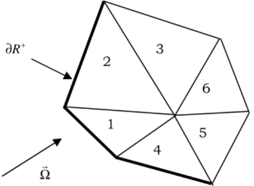
is the angular flux. The equation is closed with vacuum or reflexion boundary conditions. The triangles to be solved are sorted so that each cell is solved following a propagating front from the lightened side to the dark side of the domain.

The numerical equation solved on each triangle is:

∫

Ω − + Ω∇ + = ∂ − + T T T T e e e S n (ϕ ϕ )ψ ( . ϕ)ψ σϕψ ψ . _ r r r r (3) where T is the mesh, ∂T_the lightened boundary, ne

r

the outgoing normal to the boundary,

ψ

a basis function in the projection space (polynomial),

ϕ

the unknown angular flux to be solved, σ the total cross section of the medium, and S is the source term. Theϕe+ term is the angular flux on

the edge e from neighbour mesh (upwind flux), ϕe− is the flux of the mesh being solved. This

scheme is applied with basis functions which are polynomials of degree 0 (P0) or 1 (P1).

2.2.1 P0 solver

The flux is supposed to be constant on each mesh. An explicit expression of the flux of the being solved mesh is obtained after few calculations:

Ωr 2 1 4 5 6 3 + ∂R

(5)

4/18 V l n S l n e e e e e e e

σ

ϕ

+ Ω − + Ω − =

∑

+ − r r r r . . (4)

where some geometrical data of the cell are present like the area V.

2.2.2 P1 solver

In the linear approximation, the angular flux is represented thanks to a nodal basis. The flux is calculated at each vertex of the triangle and approximated with a linear combination of these values inside the triangle.

The flux on the triangle is found by solving a 3x3 system:

),

(

)

(

1

S

e ext e e

+

−

+

−

=

∑

_σ

−

∑

_ϕ

ϕ

M

e

T

M

e (5) with =

∫

T j iϕ ψ

M the mass matrix, =

∫

Ω∇

T

j i( . ϕ )

ψ r r

T the transport matrix, =

∫

Ω

e j i e nr ψ ϕ r . e M the

mass matrix on the incoming edge e. This non symmetric system is solved directly by Cramer’s rule.

2.3 Three dimensions elements

In 3D, the elements are not tetrahedral like in [6] but prismatic. The 2D elements are product of radial and axial basis functions. Different elements are drawn on the figure 3.

For the DGP1P0 element, flux is piecewise constant axially. The nodes are located at the middle plane of each element. The flux belongs in the P1 polynomial space (1, x, y). For the DGP1M1 element, we add an axial momentum which is linear in z and constant radially. The flux belongs in the P1 polynomial space (1, x, y, z). The DGP1P1 element is a product of P1 radial space by a P1 axial space, the flux belongs in the polynomial space (1, x, y, z, xz, yz). This last element has not been implemented yet.

− a

ϕ

Ω

r

A B C − b

ϕ

− c

ϕ

+ c

ϕ

+ a

ϕ

Figure 2. 2D triangle P1

(6)

5/18

In 3D we have twice more angular directions than in 2D, so the computing time for a DGP1P0 approximation can be estimated by multiplying the 2D-time by a factor 2Nz (Nz being the number of radial planes).

3 DSA METHOD

We detail how the DSA was implemented. The scattering is supposed to be isotropic. We followed the formalism of Adams and Martin [8]. In [6], some stability problems of this method are pointed out; they have been treated by introducing a stabilisation parameter α introduced in [10]. See [7, 11] for some presentations of the derivation of DSA. The DSA method accelerates the source iterations by estimating the error after each transport iteration. The error is approximated thanks to the diffusion operator which is a low order operator compared to the transport one. The DSA corresponds to the acceleration by diffusion, but the transport can also be accelerated by a transport operator with less angular directions (multi-grid acceleration), see [14] where it is shown to be less effective than DSA. Diffusion matrices can be used to get a diffusion solver and even a SP1 solver.

3.1 The M4S Process

The reader will find justification in [8] for the following scheme. The 2 first lines correspond to transport iteration. The 3rd one is the diffusion equation that the residual error satisfies. The superscript l+1/2 corresponds to variables calculated after one transport iteration. 1

0

+ l

F is the error to estimate thanks to the diffusion operator.

( )

r q l s l m t l m m 0 2 / 1 2 / 1 + = + ∇ ⋅ Ω _ψ + _σ_ψ + _σ _φ ₍₆₎

∑

+ + ₌ m l m m l w 1/2 2 / 1 ψ φ (7)

(

)

(

l l

)

s l s t l t F F 0 2 / 1 0 1 0 1 0 3 1 _σ _σ _σ _φ _φ σ ∇ + − = − − ⋅ ∇ + + + ₍₈₎ 1 0 2 / 1 1 + + + ₌ l ₊ l l F φ φ . (9) 3x3 Matrix 6x6 Matrix DGP1P0

{

x y z xz yz

}

B= 1, , , , , 4x4 Matrix { x y z} B= 1, , , DGP1M1 DGP1P1 { x y} B= 1, , Figure 3: 3D elements

(7)

6/18

3.2 Numerical Flux, Choice of the Stabilisation Parameter

Numerical instability appears if the discretization of the diffusion operator is not the same than the one of the transport operator [15]. In fact, consistency is a sufficient condition for stability of the DSA. So the DGFEM is used to solve the diffusion equation (D=1/3σ_t):

(

)

_∫

(

)

_∫

(

)

∫

∇ ⋅∇ − ⋅∇ + − + = + − ∂ + + K l l s K l s t K l K l v v F v F n D v F D ₀ 1 ₀ 1 σ σ ₀ 1 σ φ₀ 1/2 φ₀ (10)

The main issue here is to choose a numerical flux to compute the boundary integrals (2nd term in the equation (10)). In the transport equation, the numerical flux chosen verifies the upwind scheme. Here, a stabilisation parameter α is introduced to make the bilinear form coercive and thus to ensure the existence of a unique solution to the approximate problem. In [9], calculations show that the value of this parameter has to be in 1/h (h = stepsize) to get an elliptic form and a well posed problem. This parameter links the DGFEMs with the Interior Penalty methods which were developed independently, see [10] for references.

The numerical boundary integral is expanded as follows:

(

)

∫

[ ][ ]

∫

{

}

[ ]

∫

{

}

[ ]

∫

∂ ∂ ∂ ∂ ∇ ⋅ + ∇ ⋅ + = ∇ ⋅ − K K K K F v D n v F D n v F v F n D

α

(11)

with [u]=uext −u_int and

{ } (

)

.

2 1

int u u

u = _ext + The last term symmetrises the diffusion matrix. Wang, in [10], gives a value for the stabilisation coefficient α of one interior edge e:

(

IP

)

e κ α =max1/4, with

( )

₋ ⊥ − − + ⊥ + + + = h D p c h D p c IP e 2 2

κ . The value of the stabilisation parameter

was one issue of the modified M4S. We took c

( ) ( )

0 =c1 =2, p is the order of the polynomials.

Remarks:

-The P1 DSA is efficient to accelerate the P1 transport but the P0 DSA reduces drastically the calculation time. All calculations presented in the numerical results used the P0 DSA.

-The value of the stabilisation coefficient can be understood as choosing a boundary flux (flux on the edge) equal to the average of fluxes from both adjacent triangles whereas in the finite-volumes method, the boundary flux is a weighted average flux.

-Anisotropy of first order can be taken into account for SPn calculations.

4 PARALLELIZATION

The parallelization of the solver is necessary to reduce the computing time which may become important for large SN order. For this reason, the angular parallelization has been implemented in a first time. Two levels have been considered, the first consists in a distribution of a set of directions on each processor. For a given direction, the second level consists to perform simultaneously the calculation of different meshes along a propagation front if no dependency exists.

(8)

7/18

4.1 Distribution of the directions

For each angular direction, and for each source iteration, the angular flux is independent of the other directions with the exception of the boundary values in case of reflexive boundary conditions. So the calculations can be run simultaneously direction by direction. Indeed, the spatial resolution uses the source data estimated at the previous source iteration.

Thus, one can affect a set of angular directions by MPI process, up to one angular direction per MPI process. A set of directions is allocated to each processor. For each outer iteration and each energy group, the master processor computes the different moments of the outer source (fission and scattering from other groups) ext

lm

S . Then, for each source iteration, we perform the parallel process given (Figure 4).

4.2 Distribution of the calculation along the propagation front.

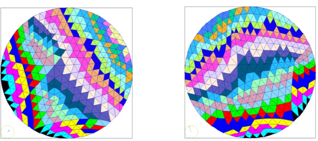
As it has been already shown, for a given direction, the calculation of the angular flux is explicit by starting from the lightened border where the angular flux is supposed to be known (zero flux or flux already calculated when symmetry condition is imposed) and then by progressing from triangle to triangle when all the lightened edges in a given triangle are known. We then calculate the different terms of a 4x4 matrix and the source term depending of the cross section and then solve the linear system, this takes about two hundred of floating point operations. A tree of dependency of the different triangles can be easily built. At each level of this tree the triangles can be computed independently. Figure 5 presents by different colors the triangles belonging in a same set of dependency and thus those which can be computed in parallel. This fine grain parallelization is achieved using OpenMP multithreading.

(9)

8/18

Using this two level parallelism, we have planned, by the end of year 2010, to compute a full 3D GENIV reactor core using around 300 energy groups and using more than 10,000 cores in few hours on the last new French petaflop machine [22].

5 CURVED TRIANGLES

A curved triangle is a triangle ABC whose one edge is an arc of a circle (BC in the Figure 6). The circle is considered because the fuel pins are cylindrical. The center of the circle O is located anywhere relatively to A. The curved triangle is supposed to be convex. The following figure displays the action of the mapping F between the curved and the straight triangle ABC and the link between curved basis functions and straight ones (one level set of the function v and one of A

A

v) are plotted in red).

5.1 Curved Basis Functions

The curved basis functions v)_iare obtained from the straight ones v and from the mapping _i

( )

K F K K F → = )

: using the formula v)_i =v_i oF−1. The action of the mapping F is detailed on

Figure 6. Mapping from straight to curved triangle.

(10)

9/18

the Figure 6. The point M'is the image of M by F. With this approach we calculate (with Mathematica) more complicated integrals on straight triangles than for straight FEM. For instance, the curved mass matrix writes:

J v v v v K j i K j i

∫

= ) ) ) (12) where J is the jacobian of F. One drawback of this approach is to find a mapping between a triangle with more than one curved side and the corresponding straight one. One possibility is to use Nurbs, but it is not done yet. We considered the straight basis functions because the number of curved sides does not change the difficulty for the computation of FEM matrices.

5.2 Straight Basis Functions

It is also possible to keep the linear usual basis functions of the straight triangle to interpolate the angular and the scalar flux on curved triangles. In this case, we calculate the integrals on more complicated geometrical domain. For instance, the curved mass matrix writes:

.

∑ ∫

∫

= + k _D j i K j i K j i k v v v v v v ) (13) k

D is the area between the straight edge and the corresponding curved one. One drawback of this

method is that the basis function corresponding to the curved edge does not vanish on this edge, so more coefficients need to be calculated in the FEM boundary matrices.

For both bases, the case of a tangent direction to the curved side needs to be treated. In fact, a tangent direction is said to be incoming or outgoing in an average sense since the criteria is the sign of the dot product between the average outer normal and the direction. So approximations are still present. We tried to refine the mesh at the tangent point, but the results were not better. One can explain it by saying that the source needs to be interpolated at the tangent point whereas it is not stored at this point, so that can prevent a better accuracy.

The straight basis functions fit less well the problems than curved ones. Numerical results on the JHR reactor confirm this view.

6 NUMERICAL RESULTS

Various numerical tests have been performed in order to verify the behavior of the solver for different core configurations. The first tests are simple one-group benchmark with very simple geometries (disk, single cell), the aim is to show the convergence ratio when the mesh size tends to zero. The second test is devoted to the classical benchmark C5G7 in order to perform a cell by cell calculation with high flux anisotropy. The third test was performed on the future JHR research reactor with a very complex geometry. The last test is devoted to the concept of ESFR (European Sodium Fast Reactor) presenting a hexagonal geometry with 33 energy group calculations. For almost all calculations, the precision on the eigenvalue was of 10-6 and the one on the flux of 10-4. All the calculations presented used DGP1M1 finite elements and were accelerated with P0 DSA: a P1 to P0 condensation is done before the diffusion step and the resulting error vector is then expanded to come back to a P1 size. But it is possible to use P1 DSA or no DSA.

(11)

10/18

6.1 h-Convergence

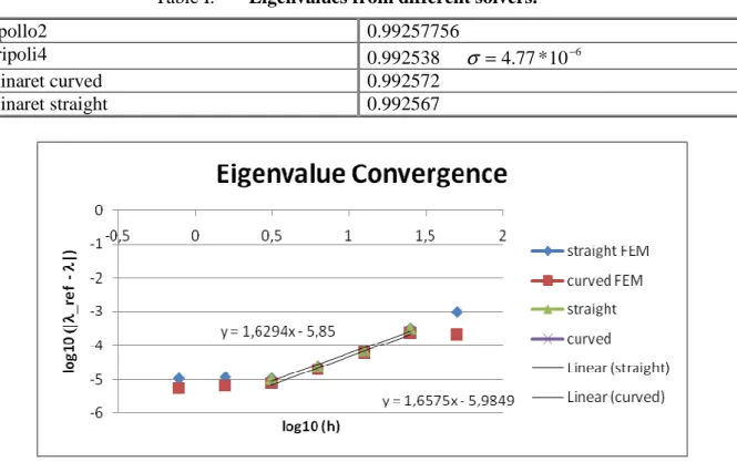
We present 2 simple cases with one energy group to enhance the h-convergence of the eigenvalue and the flux to a reference one. For the homogeneous disk the reference has been calculated by running a 1D calculation with the Apollo2 code. A Tripoli4 calculation was performed also.

6.1.1 Homogeneous disk

Calculations were made on a homogeneous disk with vacuum boundary conditions and with 528 angular directions per octant (S64). The disk radius is 50cm.

Table I. Eigenvalues from different solvers.

Apollo2 0.99257756 Tripoli4 _0.992538 6 10 * 77 . 4 − = σ Minaret curved 0.992572 Minaret straight 0.992567

The eigenvalue stops becoming closer and closer since a small difference exists between the refined eigenvalues of Apollo2 and Minaret. Curved elements do not bring any extra accuracy when the mesh is refined but results are better with coarse meshes. The rate of the eigenvalue convergence is about 1.6.

6.1.2 Large Cell

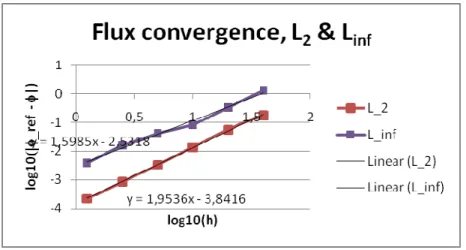
The cell consists in a square whose the edge size is 100cm and the radius of the circle within the square is 40cm. Calculations used a S16 formula with vacuum boundary conditions. We started from an unstructured mesh made of triangles whose the edge size is about 40cm. Refining the mesh consists in joining the middle points of each edge so we got triangles twice smaller. We found keff= 0.989137 for the finest mesh.

(12)

11/18

Each flux is compared to the last one which is the most accurate. Without any hypothesis of regularity of the flux, the expected rate of convergence for the L2 norm is of 1.5. So the L2 norm

converges faster but the reference value is from the same solver, so the slope may be overestimated.

6.2 C5G7 Calculations

The C5G7 Calculation is a standard OECD Benchmark proposed in 2003. We ran calculations on one eighth of the core. The power comparison with MCNP is presented in Table II and Table V. For the angular variable, the product formula seems to give better results than the level symmetric one (‘02x16’ means 2 z-levels for the polar angle and 16 radial directions for the azimuthal angle by octant). 2D calculations were made with 48901 triangles.

6.2.1 2D Calculations

Table II. C5G7 calculations with different angular curvatures

Time calculation (s) Max error (%) Average error (%) Keff

MCNP reference 1.18655 MINARET S16 1450 1.73 0.395 1.18543 MINARET 02x16 1440 1.73 0.397 1.18635 MINARET 02x16* 1660 1.84 0.403 1.18635 MINARET 02x36 2800 1.63 0.393 1.18644 MINARET 02x36* 3680 1.839 0.402 1.18644 APOLLO2 1870** 3.2 0.50 1.18636

* These calculations are similar to the ones presented above except the precision on the flux which is imposed to 10-5 instead of 10-4. From the results, increasing the precision on the flux does not bring the flux closer to the reference.

** The calculation with Apollo2 [17] was made on a Dec Alpha EV6 500MHz workstation which is twice slower than the 2.7GHz workstation we used for Minaret calculations (the S16

(13)

12/18

calculation run in 2860s on the Dec Alpha). So, for comparison, the time of Apollo2 can be divided by 2.

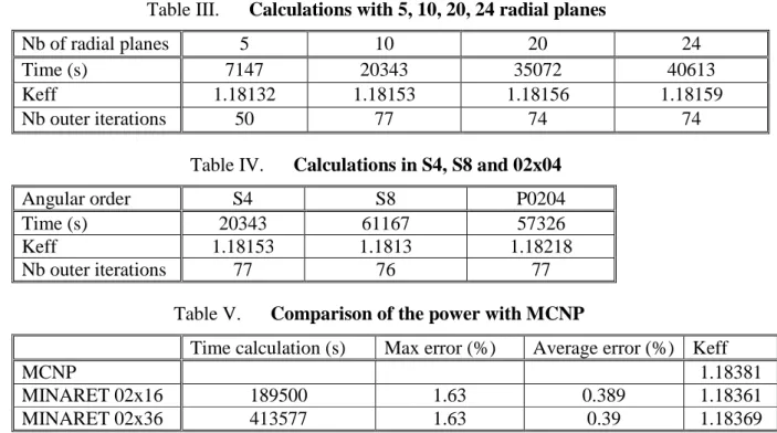
6.2.2 3D Calculations

Table III justifies we kept 10 radial planes for next calculations, and Table IV shows that product formulae are better than level symmetric ones.

Table III. Calculations with 5, 10, 20, 24 radial planes

Nb of radial planes 5 10 20 24

Time (s) 7147 20343 35072 40613

Keff 1.18132 1.18153 1.18156 1.18159

Nb outer iterations 50 77 74 74

Table IV. Calculations in S4, S8 and 02x04

Angular order S4 S8 P0204

Time (s) 20343 61167 57326

Keff 1.18153 1.1813 1.18218

Nb outer iterations 77 76 77

Table V. Comparison of the power with MCNP

Time calculation (s) Max error (%) Average error (%) Keff

MCNP 1.18381

MINARET 02x16 189500 1.63 0.389 1.18361

MINARET 02x36 413577 1.63 0.39 1.18369

In the last table, the time calculation could be reduced using parallel computations and using fewer triangles. We did not study the influence of the number of triangles in the radial planes.

6.3 JHR Calculations

To illustrate the MINARET solver capabilities, we present an application on the future European research reactor, the Jules-Horowitz-Reactor (JHR) [19], dedicated to technological irradiations. The core is composed of 34 fuel assemblies (arranged in 4 rings), 3 regions contain clustered irradiation devices (chouca regions). Each assembly is composed of 3 groups of 8 cylindrical fuel plates, maintained by three aluminum stiffeners. The core is surrounded by a beryllium reflector and a water reactor pool. The cross sections, which depend on several parameters (fuel temperature, water temperature and density, control rod insertion) are used for the whole core calculation. The physical geometry of the core is decomposed into 4149 physical regions for the radial description (see Figure 9), and 26 axial planes, this produces 53052 different regions for the complete 3D description of the core. The JHR core and assembly geometries have been described via the Graphical User Interface SILENE [21].

(14)

13/18 6.3.1 2D calculations

2D calculations ran in the TBB configuration (all rods inserted) for a starting core configuration (Figure 9). It should be noted that the high value of Keff is due to the fact that the axial buckling is not taken into account and also that the core corresponds to the beginning of cycle. The calculation corresponds to a mesh where the size of the triangles is constant inside the active part of the core and increases until the periphery (from 0.7cm to 1cm). The total number of triangles is 46986. For this calculation different FEM approximations have been compared in order to validate the curved edge FEM basis and to justify conserving volumes with straight triangles. The results are presented in Table VI.

Table VI. Comparison between different FEMs (S4 angular quadrature)

Keff Geometry : exact/approximated FEM straight/curved FEM basis 1 1.31307 approximated geometry

(volume conservation)

straight 2 1.31441 approximated geometry

(non volume conservation)

straight

3 1.31327 exact straight

4 1.31309 exact curved curved

5 1.31325 exact curved straight

The difference between lines 1 and 2 justifies conserving the volumes. Comparing lines 1 and 3 justifies using straight triangles with straight FEM (instead of curved triangles with straight FEM). For the lines 4 and 5, we ran curved FEM calculations with 2 kinds of base functions (see section 5). The curved ones seem better. From our view, curved basis functions are more consistent with the geometry.

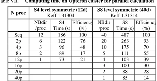
The results presented in Table VII correspond to parallel calculations with different distributions of the angular directions on the processors.

(15)

14/18

Table VII. Computing time on Opteron cluster for parallel calculation

N proc S4 level symmetric (12d)

Keff 1.31304 S8 level symmetric (40d) Keff 1.31314 NBdir /proc S4 Time (s) Efficiency (%) NBdir /proc S8 Time (s) Efficiency (%) Seq 12 186 100 40 487 100 2p 6 122 76 20 263 93 4p 3 96 48 10 175 70 8p 2 89 17 5 111 55 12p 1 73 21 4 103 39 16p 3 100 30 20p 2 88 28 40p 1 85 14

The efficiency is reduced by the increasing amount of communications (source and flux moments) and by the fact that, DSA being not parallelized, a fixed computing time is added at each source iteration.

6.3.2 3D calculations

3D calculations of the JHR core have been performed using 14 and 26 axial planes and a S4 angular quadrature. The axial geometry is given Figure 10 and results on table VIII.

Table VIII. 3DCalculations with different number of planes

Nb of planes / SN order 14 (S4) 26 (S4) 26 (S8)

Time(s) / Nb proc. 2645 (4p) 3719 (4p) 5441 (8p)

keff 1.25652 1.25697 1.25704

Nb outer iterations 26 22 22

The time with 26 planes in S4 with one processor was 12500s.

Figure 10. Axial description of the JHR core

Water

Shielding zone _{Shielding zones}

Core

(16)

15/18

6.4 ESFR calculations

The ESFR concept (European Sodium Fast Reactor) takes place in the fourth generation reactors project. The map of the core is given on figure 11. It consists into 17 rings of assembly. The inner and outer fuel regions have different Pu mass content. There are 225 inner fuel subassemblies and 228 outer fuel sub-assemblies. The control rod system is composed of 9 DSD (Diverse Shutdown Device) and 24 CSD (Control and Shutdown Device). The material cross sections coming from ECCO library are homogenized in a 33 energy multi-group discretization. The material distribution is given on Figure 11

Minaret calculations have been performed considering the steady state solution. The following options have been used: each hexagon is split into 14 triangles, axially a mesh measures 20cm in fuel and reflector, giving 11 planes. The total number of elements is 11438 in 2D and 125813 for the 3D calculation.

In Table IX and Table X are reported all the results performed on the whole ESFR core for a 2D and 3D configuration. The tests have been performed with S4 and S8 level symmetric quadrature on a cluster platform composed by 40 nodes of Opteron2.8 Ghz octo-processors, with compiler gcc 4.1.1. The tables show the good scalability by increasing the number of processors even if the DSA parts have not been yet parallelized.

Figure 11. ESFR Axial and Radial material and calculation geometry description

DSD CSD

Inner Fuel Outer Fuel

(17)

16/18

Table IX. ESFR 2D Parallel calculations on cluster computer S4 level symmetric (12d) Keff 1.04271 S8 level symmetric (40d) Keff 1.04272 N proc NBdir /proc S4 Time (s) Efficiency (%) NBdir /proc S8 Time (s) Efficiency (%) Seq 12 229 100 40 690 100 2p 6 137 84 20 365 95 4p 3 95.5 60 10 216 80 8p 2 76.4 37 5 126 68 12p 1 4 111 52 16p 3 98 44 20p 2 87 40 40p 1 72 24

Table X. ESFR 3D Parallel calculations on cluster computer

7 CONCLUSION

MINARET is a deterministic unstructured SN multi-group transport solver parallelized with respect to the angular directions. It solves the steady state Boltzmann equation. It has been developed within the Apollo3 frame gathering several other solvers. It is possible to run core calculations by meshing the whole core with the only constrain to get a 3D cylindrical mesh. The 2D basis mesh is composed by a collection of conforming triangles.

The DSA method reduces time calculations by a factor 3 (at least) on all the tested reactors. The DSA matrices are the only matrices stored by the solver. Indeed, for transport calculations, the 4x4 (in 3D) transport matrices are recalculated for each cell and for each iteration.

S4 level symmetric (24d) Keff 1.00389 S8 level symmetric (80d) Keff 1.00397 N proc NBdir /proc S4 Time (s) Efficiency (%) NBdir /proc S8 Time (s) Efficiency (%) Seq 24 13534 100 80 43334 100 2p 12 7615 89 40 23156 94 4p 6 4370 77 20 11862 91 8p 3 2718 62 10 6454 84 12p 2 2394 47 / / 24p 1 1852 30 / / 16p 5 3845 70 20p 4 3588 60 27p 3 3349 48 40p 2 2963 37 80p 1 2195 25

(18)

17/18

The approximation of the geometry by straight triangles with linear finite elements is acceptable if volumes are preserved. So, curved elements may not be necessary since they slow down calculations. However, curved elements can be used to mesh the fuel cells discretized into sectors using fewer curved triangles than with straight triangles. In this case, triangles with several curved edges are necessary. FEM on that kind of elements are made possible thanks to NURBS. That will be the next step.

Parallelization according to the angular directions speeds up calculation. The solver shows good scalability for small numbers of processors. For large number of processors, the DSA step reduces the efficiency because it is not yet parallelized. Parallelization using the domain decomposition method could be implemented to address this problem.

Future projects are first the extension to kinetics calculations and also to extend the solver to non conforming elements and to tetrahedral meshes. In the immediate future, we intend to use higher order elements.

8 ACKNOWLEDGMENTS

Authors want to thank their colleagues of their lab for the help they provided, and thank also the CEA for funding their work.

9 REFERENCES

1. W. H. REED and T. R. HILL, “Triangular Mesh Methods for Neutron Transport Equation,”

LA-UR-73-479, Los Alamos Scientific Laboratory, 1973.

2. P. LESAINT and P. A. RAVIART, “On a Finite Element Method for Solving the Neutron

Transport Equation,” Mathematical Aspects of Finite Elements in Partial Differential

Equations, p. 89, C. A. DE BOOR, Ed., Academic Press, New York, 1974.

3. C. JOHNSON and J. PITKARANTA, “Convergence of a Fully Discrete Scheme for

Two-Dimensional Neutron Transport,” SIAM J. Numer. Anal., 20, 5, p.951, Oct. 1983.

4. T.E. PETERSON, “A Note on the Convergence of the Discontinuous Galerkin Method for a

Scalar Hyperbolic Equation,” SIAM J. Numer. Anal., 28, 1, p.133, Feb. 1991.

5. D.N. ARNOLD, F. BREZZI, B. COCKBURN, and D. MARINI, “Discontinuous Galerkin methods for elliptic problems”, Discontinuous Galerkin Methods. Theory, Computation and

Applications, B. Cockburn, G.E. Karniadakis, and C.-W. Shu, eds., Lect. Notes Comput. Sci. Eng. 11, Springer-Verlag, Berlin, 2000, pp. 89–101.

6. T. A. WAREING, J. M. McGHEE, J. E. MOREL, S. D. PAUTZ, “Discontinuous Finite Element Sn Methods on Three-Dimensional Unstructured Grids,” Nucl. Sci. Eng., 138,

p.256, 2001.

7. J. S.WARSA, T. A.WAREING, and J. E. MOREL, “Fully Consistent Diffusion Synthetic Acceleration of Linear Discontinuous SN Transport Discretizations on Unstructured Tetrahedral Meshes,” Nucl. Sci. Eng., 141, p.236, 2002.

8. M. L. ADAMS and W. R. MARTIN, “Diffusion Synthetic Acceleration of Discontinuous Finite Element Transport Iterations,” Nucl. Sci. Eng., 111, p.145, 1992.

9. D. N. ARNOLD, “An interior penalty finite element method with discontinuous elements,”

(19)

18/18

10.Y. WANG, ‘Adaptive Mesh Refinement Solution Techniques for the Multi-group SN Transport Equation Using a Higher-Order Discontinuous Finite Element Method’, PhD Thesis, Texas A&M University (2009).

11.M. L. ADAMS, E. W. LARSEN, “Fast iterative methods for discrete-ordinates particle transport calculations,” Prog. in Nuclear Energy, 40, 1, p.3, 2002.

12.D. S. LUCAS et al, “Applications of the 3-D Deterministic Transport Attila® for Core Safety Analysis,” Americas Nuclear Energy Symposium 2004

13.J. RAGUSA and Y.WANG, “A High-Order Discontinuous Galerkin Method for the SN

Transport Equations on 2D Unstructured Triangular Meshes,” Ann. Nucl. Eng., 36, p.931,

2009.

14.E. M. GELBARD, L. A. HAGEMAN, “The Synthetic Method as Applied to the Sn Equations,” Nucl. Sci. Eng., 37, p.288, 1969

15.R. E. ALCOUFFE, “Diffusion Synthetic Acceleration Methods for the Diamond-Differenced Discrete-Ordinates Equations,” Nucl. Sci. Eng., 64, p.344, 1977

16.G. KANSCHAT, Discontinuous Galerkin Methods for Viscous Incompressible Flow, Deutscher University Springer Verlag, Wiesbaden, Germany, 2007.

17.F.MOREAU et al, ‘CRONOS2 and APOLLO2 results for the NEA C5G7 MOX benchmark’,

Prog. in Nuclear Energy, 45, 2-4, pp. 179-200, 2004

18.A. ERN, J-L. GUERMOND, Theory and Practice of Finite Elements, Springer, New York (2004).

19.D. Iracane, Proceedings TRTR-2005/IGORR-10 Joint meeting: The Jules Horowitz Reactor, a new Material Testing Reactor in Europe, Gaitherburg, Maryland (USA), September 12-16, 2005.

20.H. Golfier,R. Lenain, C. Calvin, J-J. Lautard, A-M. Baudron, Ph. Fougeras, Ph. Magat, E. Martinolli, Y. Dutheillet, “APOLLO3: a common project of CEA, AREVA and EDF for the development of a new deterministic multi-purpose code for core physics analysis”,

International Conference on Mathematics, Computational Methods & Reactor Physics, Saratoga Springs, New York, May 3-7, (2009).

21.Zarko Stankovski "La Java de Silène" A graphical user interface for 3D pre & post processing: state-of-the-art and new developments. Proceeding of M&C 2011, Rio de Janeiro, May 08-12.

22.J.J. Lautard, E. Jamelot, J. Dubois, C. Calvin, A.M.Baudron "Parallelization of 3D transport solvers within APOLLO3 code" this meeting Proceeding of M&C 2011, Rio de Janeiro, May 08-12.