HAL Id: tel-00556902
https://tel.archives-ouvertes.fr/tel-00556902
Submitted on 18 Jan 2011HAL is a multi-disciplinary open access archive for the deposit and dissemination of sci-entific research documents, whether they are pub-lished or not. The documents may come from teaching and research institutions in France or abroad, or from public or private research centers.
L’archive ouverte pluridisciplinaire HAL, est destinée au dépôt et à la diffusion de documents scientifiques de niveau recherche, publiés ou non, émanant des établissements d’enseignement et de recherche français ou étrangers, des laboratoires publics ou privés.
linked to environmental fluctuations. From imaging
systems to size-based models.
Pieter Vandromme
To cite this version:
Pieter Vandromme. Decadal evolution of the Ligurian Sea zooplankton linked to environmental fluc-tuations. From imaging systems to size-based models.. Ocean, Atmosphere. Université Pierre et Marie Curie - Paris VI, 2010. English. �tel-00556902�
L
O
V
-
-M
LOV UMR7093
T
HÈSE
présentée en vu d’obtenir le grade de Docteur, spécialité Science de l’environnement — Océanographie
par
Pieter Vandromme
É
VOLUTION DÉCENNALE DU ZOOPLANCTON DE LA
M
ER
L
IGURE EN RELATION AVEC LES FLUCTUATIONS
ENVIRONNEMENTALES
. D
E L
’
IMAGERIE À LA
MODÉLISATION BASÉE EN TAILLE
.
—
D
ECADAL EVOLUTION OF
L
IGURIAN
S
EA ZOOPLANKTON
LINKED TO ENVIRONMENTAL FLUCTUATIONS
. F
ROM
IMAGING SYSTEMS TO SIZE
-
BASED MODELS
.
Thèse soutenue le 26 Novembre 2010 devant le jury composé de :
Pr. LOUISLEGENDRE (Président)
Dr. JEAN-HENRIHECQ (Rapporteur)
Dr. MARIA-GRAZIAMAZZOCCHI (Rapportrice)
Pr. VICTORSMETACEK (Examinateur)
Dr. LARSSTEMMANN (Directeur)
Pr. GABYGORSKY (Directeur)
L
O
V
-
-M
LOV UMR7093
T
HÈSE
présentée en vu d’obtenir le grade de Docteur, spécialité Science de l’environnement — Océanographie
par
Pieter Vandromme
É
VOLUTION DÉCENNALE DU ZOOPLANCTON DE LA
M
ER
L
IGURE EN RELATION AVEC LES FLUCTUATIONS
ENVIRONNEMENTALES
. D
E L
’
IMAGERIE À LA
MODÉLISATION BASÉE EN TAILLE
.
—
D
ECADAL EVOLUTION OF
L
IGURIAN
S
EA ZOOPLANKTON
LINKED TO ENVIRONMENTAL FLUCTUATIONS
. F
ROM
IMAGING SYSTEMS TO SIZE
-
BASED MODELS
.
Thèse soutenue le 26 Novembre 2010 devant le jury composé de :
Pr. LOUISLEGENDRE (Président)
Dr. JEAN-HENRIHECQ (Rapporteur)
Dr. MARIA-GRAZIAMAZZOCCHI (Rapportrice)
Pr. VICTORSMETACEK (Examinateur)
Dr. LARSSTEMMANN (Directeur)
Pr. GABYGORSKY (Directeur)
J
E tiens tout d’abord à remercier mes superviseurs qui ont rendu ce travail possible. Ces 3 anspassés à travailler à vos côtés furent extrêmement enrichissants, aussi bien au niveau scientifique
qu’humain, merci d’avoir partagé votre savoir et de m’avoir permis de vivre une thèse aussi remplie.
Je remercie tout particulièrement Lars Stemmann pour sa sympathie, ses idées, pour le temps passé à
m’encadrer au jour le jour et pour l’avoir si bien fait. Gaby Gorsky pour sa vision de la science et pour
les nombreux sobriquets dont il m’a affublé. Et aussi Jean-Marc Guarini, mon troisième directeur,
pour ses idées toujours très enrichissantes.
Merci aussi à Victor Smetacek, Louis Legendre, Maria-Grazia Mazzocchi et Jean-Henri Hecq
pour avoir accepté d’être membres de mon jury et particulièrement à Maria-Grazia et Jean-Henri
pour avoir évalué ce travail dans le détail et donc lu ces presque 200 pages. Merci !
Ce travail n’aurait pas été possible sans l’aide des nombreux membres de l’équipe, présent ou
passé, avec qui j’ai eu la chance de travailler, principalement Marc Picheral, Léo Berline, Carmen
Garcia-Comas Rubio, Corinne Desnos, Franck Prejger, Steven Colbert, Ornella Passafiume, Lionel
Guidi, Stéphane Gasparini, Laure Mousseau, les nombreux stagiaires à avoir travaillé sur le ZooScan
et le PVM, et beaucoup d’autres que je remercie énormément !
Je n’aurais pas pu non plus réaliser une partie de ce travail, et pas la moindre, sans avoir eu la
chance de collaborer avec l’équipe Comore de l’INRIA de Sophia-Antipolis: Éric Benoît, Jonathan
Raultet Jean-Luc Gouzé ! Je vous remercie pour ces très bons moments passés à Sophia et pour ce
savoir acquis en mathématique et modélisation ! J’espère que cette collaboration ne s’arrêtera pas là
et Jonathan, bon courage pour ta dernière année de thèse !
Polarsternpour fertiliser l’Océan Atlantique Sud à coup de sacs de poudre de fer ! Vivre 70 jours au
milieu des icebergs et des albatrosses à apprendre et partager tant de choses fut une des meilleures
expériences de ma vie. Alors merci à Wajih Naqvi et Victor Smetacek pour m’avoir accueilli dans
ce projet et à Maria-Grazia Mazzocchi pour m’avoir accueilli dans l’équipe zooplancton. Être
re-mercié deux fois n’est pas de trop ! La place manque ici pour remercier les 47 autres scientifiques
présents (plus ceux rencontrés au séminaire à Goa qui ont aussi participés à ce projet) et les presque
50 membres d’équipage, cependant il ne serait pas correct d’oublier le Capitaine Schwarz.
Mais au boulot, il n’y a pas que le boulot, et je remercie donc toutes les personnes passées par
le laboratoire de Villefranche-sur-Mer, particulièrement ceux dont j’ai partagé le bureau (la crique
et l’open space), et qui en ont rendus la vie drôle, festive et amicale ! Coco charnel, Marc, Léo,
Francky, Ornella, Martina Tartina, Christophe, Mika, Martinouschka, Carmen, Jean-Baptiste, Steevie
et sa baronne, Sasha, François le Beatnik, Noémie, Rizou, Samir Alliouâne, La mère maquerelle, les
nombreux scientifiques, techniciens, stagiaires, doctorant, CDD à être passé par là, Les Master des
différentes promo, tout ceux qui râleront de ne pas avoir été mentionnés et encore beaucoup d’autres
qui de toute façon ne liront jamais ces lignes donc c’est pas trop grave si ils n’y sont pas !
Ce travail, ainsi que le bon fonctionnement du laboratoire, ne serait pas possible sans l’aide et la
patience de tout les membres de l’administration et des services du Laboratoire : Isabelle, Corinne,
Manuelle, Susy, Martine, Thierry, Didier, Danièle, Cécile, Alejandra, Laurent, Olivier, Stéphane,
Jean-Yves, Jean-Luc, Fabrice, Alain. . .
Et, bien évidemment, Louis Legendre et Antoine Sciandra, directeur du LOV et Fauzi Mantoura
locaux.
Finalement, je gardais le meilleur, je remercie mes amis et ma famille (avec une mention spéciale
pour ma mère) pour m’avoir toujours soutenus, aidés et d’être là ! Merci !
à Villefranche-sur-Mer, le 26 Novembre 2010.
Pieter Vandromme
Le suivi à long terme de la baie de Villefranche-sur-Mer et le développement de méthodes
d’imagerie pour l’analyse du zooplancton ont apporté une grande quantité d’informations permettant
de mieux comprendre les écosystèmes marins, et ceux de la mer Ligure en particulier. La présente
thèse représente une partie de ce suivi. L’objectif principal était de mieux comprendre — grâce à
une analyse conjointe de divers ensembles de données, une évaluation des méthodes de mesure et la
modélisation — la dynamique à long terme du zooplancton et ses liens directs avec l’environnement
biologique et physique ainsi qu’avec les indicateurs du climat mondial.
Dans la première partie, « Identification de nouveaux biais dans les spectres de taille dérivés
de l’image », chapitreII, nous avons évalué la validité des systèmes d’imagerie comme outils pour
mesurer la taille de la structuration des communautés de zooplancton. Plus de 20 échantillons (plus
13 sur le filet Régent) ont été analysés au maximum d’efforts possible, c’est à dire avec une
sépara-tion manuelle des objets en contact sur la vitre du scanner, puis avec une séparasépara-tion numérique de
ces objets restants, suivi d’une classification visuelle complète. Les effets de différents biais sur les
spectres de taille du zooplancton ont été ensuite examinés. Ces biais ont été produits par le contact des
objets les uns avec les autres lors de l’acquisition des images, l’efficacité de la classification
automa-tique et le fait d’utiliser un modèle unique au lieu d’un modèle basé sur la taxonomie pour calculer
les biovolumes et les biomasses. Il a été constaté qu’il est nécessaire de séparer manuellement les
échantillons avant l’acquisition des images sur le plateau du scanner, que la classification
automa-tique n’est efficace que pour les classes de taille les plus abondantes du groupe le plus abondant et,
par conséquent, qu’une correction visuelle est nécessaire au moins pour les plus grands organismes.
Enfin, les disparités taxonomiques et/ou de forme en fonction de la taille des échantillons analysés
étaient trop petites pour détecter une différence dans l’utilisation d’un modèle unique ou d’un modèle
paru que l’utilisation de systèmes d’imagerie, tel que le ZooScan, sans séparation manuelle d’objets
ni, entre autres, de correction de la séparation manuelle, peuvent donner un spectre de taille incorrect.
Il est par conséquent nécessaire d’y passer du temps. Toutefois, les systèmes d’imagerie permettent
un traitement rapide des échantillons et fournissent une quantité importante de données, à la fois sur
la distribution des tailles et sur la taxonomie.
Dans la deuxième partie, « La variabilité inter-annuelle des écosystèmes de la mer Ligure »,
chapitreIII, nous avons exploré la période 1995-2005 de la baie de Villefranche-sur-Mer. Cette
péri-ode était la plus riche en données disponibles. Nous avons ensuite analysé conjointement le
zooplanc-ton, l’hydrologie à partir des données de sonde CTD (température, salinité, densité), les éléments
nutritifs et le phytoplancton à partir des échantillons des bouteilles Niskin (nitrates, phosphates,
sil-icates, chlorophylle-a), les particules en suspension à partir des mêmes bouteilles analysées avec un
Coulter Coulter (distribution de taille de 3 à 90 µm), les conditions météorologiques mesurées au
Sémaphore, situé à 1,2 km du site de surveillance (température, précipitations, irradiation) et le
cli-mat mondial (NHT, NAO, ENSO, AO, AMO). Le zooplancton a été échantillonné chaque semaine
avec un filet WP2 allant de 60 m à la surface et les échantillons ont été analysés avec le ZooScan.
Une classification visuelle en 9 groupes zooplanctoniques des grands organismes a été faite (> 0,724
mm3) et les petits copépodes issus de la classification automatique ont été utilisés (10 groupes au
total). Nous avons observé un changement de régime de faible à forte abondance de presque tous
ces groupes aux environs de l’an 2000, avec un décalage d’environ 2 ans entre les petits copépodes
et les plus grands. Ce changement semble infirmer les tendances prévues vers une oligotrophie ainsi
que les antagonismes entre certains groupes comme les copépodes, les chaetognathes et les méduses.
On est frappé par la tendance clairement opposée entre les nitrates et le zooplancton par rapport à
la chlorophylle-a. Un fort broutage semble contrôler le phytoplancton. Cela a des implications dans
sur-Mer et de ses fluctuations à long terme. Les principaux forçages de la variabilité inter-annuelle
observée sont la force de la convection hivernale et le rayonnement solaire printanier et estival. La
force de la convection hivernale est déterminée par la température et les précipitations d’hiver. La
convection hivernale détermine le mélange et donc la remise en suspension des éléments nutritifs
qui affecte le réseau trophique par un contrôle « bottom-up ». L’irradiation solaire printanière et
estivale semble également jouer un rôle déterminant dans la dynamique inter-annuelle. Elle est
forte-ment corrélée au zooplancton et a la possibilité d’inverser l’effet de la convection hivernale dans les
deux sens (observé en 1995, 1999 et 2001). Nous supposons que cela joue sur la disponibilité de la
lumière pour la croissance du phytoplancton. Enfin, des corrélations avec les indicateurs du climat
apparaissent seulement sur une période plus longue, à savoir de 1960 à 2008. Quelques liens ont été
constatés entre la température de l’hémisphère Nord (NHT) et l’oscillation Nord Atlantique (NAO)
avec les précipitations et salinité en hiver, et entre l’oscillation multidécennale de l’Atlantique (AMO)
et l’irradiation printanière et estivale.
Puis dans la dernière partie, « Modélisation continue du zooplancton basée sur la taille », chapitre
IV, nous avons développé un modèle continu basé sur la taille de la dynamique du zooplancton. Les principaux objectifs du développement de ce modèle sont d’étudier les moyens possibles d’améliorer
la représentation du zooplancton dans les modèles et de faire fonctionner le modèle avec les données
mesurées localement. Il a été choisi de développer un modèle basé sur la taille car de nombreux
processus physiologiques et inter-individuels sont proportionés à la taille. Par conséquent, le fait de
ne considérer qu’une structuration de taille permet de réduire le nombre de paramètres. Ces modèles
permettent également d’étudier une dynamique complexe. Le modèle actuel est un modèle continu
basé sur la taille de la dynamique du zooplancton, c’est-à-dire que la formulation ne tient pas compte
des classes de taille, et intègre une formulation du broutage, de la prédation, de la croissance, de la
(le taux de croissance) et la sortie est le spectre de taille du zooplancton sur lequel nous avons mesuré
le biovolume total et la pente log-linéaire. Un point clé du modèle est d’utiliser un cas mathématique
particulier pour assurer certaines propriétés mathématiques et réduire le nombre de paramètres qui
doivent être définis. Le cas particulier est appelé « cas infini » sur lequel le spectre est infini dans les
deux sens. Dans ce cas il n’y a pas de phytoplancton et aucune mortalité exterieur : nous étendons la
formulation de prédation à l’infini ; dans ce cas, la prédation sur l’extension du côté gauche est utilisée
pour calculer l’affinité de broutage, de même, la prédation sur l’extension du côté droit est utilisée
pour calculer les taux de mortalité exterieur. En étudiant les solutions pour atteindre un équilibre
allométrique, nous avons réduit le nombre de paramètres de 13 à 7. La comparaison avec les données
a été faite sur les deux scénarii principaux identifiés dans le chapitre précédent. Pour calculer l’entrée
du modèle, à savoir le taux de croissance du phytoplancton, nous avons utilisé un modèle déjà mis
au point pour le même endroit. Pour l’instant seule une optimisation de base a été réalisée. Il semble
qu’en changeant seulement deux paramètres de leurs valeurs types obtenues dans la littérature, nous
sommes en mesure de représenter assez bien la dynamique observée du zooplancton, notamment
une forme saisonnière particulière de la dynamique des pentes des spectres de taille ainsi que la
saisonnalité du biovolume de zooplancton. Cela tend à confirmer que les modèles basés sur la taille
du zooplancton sont efficaces pour représenter des dynamiques réalistes et complexes en utilisant un
nombre limité de paramètres.
Beaucoup de débouchés se dégagent de ce manuscrit, dont certains sont présentés dans les
dis-cussions générales (chapitre V). Notamment, la série temporelle de zooplancton a été étendue avec
des échantillons récemment traités afin de couvrir la période 1966-2010, soit 45 années de données
avec une haute résolution temporelle. Cette série temporelle apparaît comme l’une des plus longues
dans le monde. En utilisant les résultats obtenus, en particulier ceux du chapitre III, nous avons
l’environnement physique de la baie de Villefranche-sur-Mer. Quelques premières observations et
hypothèses sont présentées à la fin du manuscrit.
Long-term monitoring of the bay of Villefranche-sur-Mer and development of new imaging
method-ologies to analyze zooplankton have brought about large amount of knowledge in the comprehension
of marine ecosystems and of the Ligurian Sea. This thesis is a part of it. The main objective was —
through joint analysis of various datasets, methodology assessment and modeling — to better
under-stand the long-term dynamics of the zooplankton and its links with the direct biological and physical
environment as well as with global climate indicators.
In the first part (“Identifying new biases from image-derived size spectra”, chapter II) we have
assessed the validity of imaging systems as tools to measure the size structuration of zooplankton
communities. More than 20 samples (plus 13 from the Régent net) were analyzed with maximum
effort, i.e., with manual separation of touching objects on the scanning tray, with numerical separation
of remaining touching objects and with complete visual classification. The effect of different biases on
the zooplankton size spectra were then investigated. These biases were the effects of objects in contact
with each other during the image acquisition, the efficiency of the automatic classification and the
effect of using a single model instead of a taxon-based one to calculate biovolumes and biomasses. It
was found that it is needed to separate manually samples before the image acquisition on the scanning
tray. Then that the automatic classification is efficient only for the most abundant size classes of the
most abundant group, hence a visual correction is needed for at least the largest organisms. Finally,
size dependent taxonomic and/or shapes differences were too small within the samples analyzed to
detect some variations in using a single model or a taxon-based model of converting individual size
to biovolume/biomass. It appeared that using imaging systems such as the ZooScan without manual
separation of objects and correction of the manual separation, among others, can lead to incorrect size
of samples and provide a rich amount of data, both on size distribution and on taxonomy.
In the second part (“Inter-annual variability of the Ligurian Sea pelagic ecosystem”, chapterIII)
we have explored the time period 1995-2005 of the bay of Villefranche-sur-Mer. This period was the
richest according to available datasets. We have then jointly analyzed the zooplankton, the hydrology
from CTD casts (temperature, salinity, density), the nutrients and phytoplankton from Niskin bottles
(nitrates, phosphates, silicates, chlorophyll-a), the suspended particles from Niskin bottles and
ana-lyzed with the Coulter Counter (size distribution from 3 to 90 µm), the weather from the Sémaphore
station 1.2 km away from the monitoring site (temperature, precipitations, irradiation) and the global
climate (NHT, NAO, ENSO, AO, AMO). The zooplankton was sampled weekly with a WP2 net from
60 m to surface, and samples were analyzed with the ZooScan. A visual classification in 9
zooplank-tonic groups of larger organisms was made (>0.724 mm3) and smaller copepods from automatic
classification were used (total of 10 groups). We found a shift from low to high abundances of nearly
all groups ca. 2000, with a time-lag of about 2 years between small copepods and larger groups.
This shift seems to invalidate predicted trends toward oligotrophy as well as antagonisms between
some groups like copepods, chaetognaths and jellyfish. A striking result was the clear opposite trend
on inter-annual time scale of nitrates and zooplankton vs. chlorophyll-a. A strong grazing seems to
control the phytoplankton. This has some implications in using chlorophyll-a as an indicator of the
trophic state of the bay of Villefranche-sur-Mer and its long-term fluctuations. The main forcings of
the observed inter-annual variability were the strength of the winter convection and the solar
irradi-ation in spring / summer. The strength of the winter convection is determined by winter temperature
and precipitations. The winter convection will determine the mixing and hence the nutrients
replen-ishment that will ultimately affect larger organisms through a “bottom-up” control. Yet, the spring
/ summer solar irradiation also seems to play a determining role in the inter-annual dynamics. It is
vection in both directions (observed in 1995, 1999 and 2001). We hypothesized that it plays on the
light availability for the phytoplankton growth. Finally, correlations with climate indicators were only
found on a longer time scale, i.e. from 1960 to 2008. Some links were pointed out between the North
Hemisphere Temperature (NHT), the North Atlantic Oscillation (NAO) and precipitations and
salin-ities in winter, and between the Atlantic Multidecadal Oscillation (AMO) and the spring / summer
solar irradiation.
Then in the last part (“Continuous size-based modeling of zooplankton”, chapterIV) a
continu-ous size-based model of zooplankton dynamics is developed. The major aims of developing a model
were to explore possible ways of improving the representation of zooplankton in models and to run
the model with locally-measured data. It was chosen to develop a model based on size because many
physiological and inter-individuals processes scale with size, hence considering only a size
structura-tion will reduce the numbers of parameters. Such models also allow a complex dynamics. The present
model is a continuous size-based model of zooplankton dynamics, i.e., the formulation does not
con-sider size classes, and includes grazing, predation, growth, external mortality and reproduction. The
entry of the model is the energy created by the phytoplankton (the growth rate) and the output is the
size spectrum of the zooplankton on which we measured the total biovolume and the log-linear slope.
A key point of the model is the use of a particular mathematical case to ensure some mathematical
properties and reduce the number of parameters that need to be set. The particular case is called the
“infinite case” on which the spectrum is infinite in both directions. In this case there is no
phytoplank-ton and no external mortality: we extended the predation formulation to infinity and then predation
upon the extended left side was used to calculate the grazing affinity; it is similar to the right side on
which the predation by the right extension was used to compute the external mortality rates. By
look-ing at solutions for an allometric equilibrium we reduced the number of parameters from 13 to 7. The
To compute the entry of the model, i.e., the growth rate of phytoplankton, we used a model
previ-ously worked out for the same location. Up to know only a basic optimization has been performed. It
appears that by changing only two parameters from their typical values obtained from literature we
are able to represent fairly well the observed dynamics of the zooplankton in the two main scenarii,
notably a particular seasonal shape of the dynamics of the slopes as well as the seasonality of total
biovolume of zooplankton. This tends to confirm that size-based models of zooplankton are efficient
to represent realistic and complex dynamics with a limited number of parameters.
Many prospects emerge from this manuscript, some of them are presented in the general
discus-sions (chapterV). In particular, the time series of zooplankton was extended with recently processed
samples to cover the period 1966-2010, i.e., 45 years of data with a high temporal resolution. This
time series appears as one of the longest in the world. Using findings from mainly chapter III we
started analyzing this time series in a context of long-term changes in the physical environment of the
bay of Villefranche-sur-Mer. Some first observations and hypotheses are presented at the end of the
manuscript.
CONTENTS xxi
LIST OFFIGURES xxv
LIST OFTABLES xxxiii
I GENERAL INTRODUCTION 1
I.1 ZOOPLANKTON CHANGES IN THEMEDITERRANEANSEA . . . 4 I.2 SIZE-BASED ANALYSIS AND MODELING OF THE ZOOPLANKTON . . . 7 I.2.1 Meaning of size for zooplankton . . . 8 I.2.2 Measuring the size . . . 11 I.2.3 Size-based theory and models . . . 12 I.2.4 Incorporating size in models . . . 18 I.3 METHODS . . . 23 I.3.1 Localization of the sampling site . . . 23 I.3.2 Imaging procedure . . . 26 I.3.2.1 Samples used . . . 26 I.3.2.2 Imaging procedure . . . 26 I.3.2.3 Automatic classification of objects . . . 28 I.3.2.4 Size-spectra computation . . . 30 I.3.3 Statistical analyses . . . 31 I.3.3.1 Identifying regime shifts . . . 32 I.3.3.2 Computing distances between size spectra . . . 36 I.4 ORGANIZATION OF THE THESIS . . . 38
II IDENTIFYING NEW BIASES FROM IMAGE-DERIVED SIZE SPECTRA 41
II.1 INTRODUCTION TO BIASES FROM IMAGE ANALYSIS OF ZOOPLANKTON . . . 43
II.2 DATA USED . . . 46 II.3 IDENTIFYING NEW BIASES . . . 47 II.3.1 Plankton selection by nets . . . 48 II.3.2 Impact of touching objects (TO) on the shape of zooplankton observed spectrum . . 50 II.3.3 Biases on the shape of the predicted spectrum from automatic classification . . . . 54
II.4 CONCLUSION . . . 62
III INTER-ANNUAL VARIABILITY OF THELIGURIANSEA PELAGIC ECOSYSTEM 67 III.1 INTRODUCTION. . . 69 III.2 DATASETS USED . . . 70 III.3 RESULTS . . . 73 III.3.1 Statistical analysis . . . 74
III.3.1.1 Links between parameters using Principal Components Analysis (PCA) . . . 75 III.3.1.2 Identification of shifts using STARS . . . 79 III.3.1.3 Classification of years according to size spectra and the modified
Hausdorff distance . . . 80 III.3.1.4 Correlations between annual anomalies . . . 82 III.3.2 Descriptive analysis . . . 84 III.3.2.1 Zooplankton community dynamics . . . 85 III.3.2.2 Crustacean size structure . . . 88 III.3.2.3 Environmental variability . . . 88 III.4 DISCUSSION . . . 98
III.4.1 Winter forcing on the ecosystem . . . 98 III.4.2 Effect of spring / summer irradiation and other patterns . . . 104 III.4.3 Conceptual schematic . . . 105 III.4.4 Links with Global Climate indicators . . . 108 III.5 CONCLUSION . . . 113
IV CONTINUOUS SIZE-BASED MODELING OF ZOOPLANKTON 117
IV.1 INTRODUCTION TO ZOOPLANKTON MODELS OF THENW MEDITERRANEANSEA 119 IV.2 PRESENTATION OF THE CONTINUOUS SIZE-BASED MODEL . . . 123 IV.2.1 Ecological conceptual scheme . . . 123 IV.2.2 Mathematical formulation . . . 124 IV.2.2.1 General case . . . 124 IV.2.2.2 Infinite case . . . 127 IV.2.3 Discussion on model formulation . . . 132 IV.2.3.1 Grazing, predation and growth . . . 132 IV.2.3.2 Mortality on zooplankton . . . 135 IV.2.3.3 Closure on reproduction . . . 135 IV.2.3.4 Phytoplankton dynamics . . . 136 IV.2.4 Values for parameters . . . 136 IV.3 BEHAVIOR OF THE MODEL. . . 139
IV.4 COMPARISON WITH OBSERVATIONS . . . 148 IV.4.1 Integration of a phytoplankton growth model . . . 149 IV.4.2 Data presentation . . . 150 IV.4.3 Comparison with default parameters . . . 153 IV.4.4 Preliminary results of optimization . . . 155 IV.5 CONCLUSION& PERSPECTIVES. . . 159
V GENERAL DISCUSSION AND PERSPECTIVES 163
V.1 MEASUREMENT OF SIZE SPECTRA FROM IMAGING METHODS . . . 165 V.2 FLUCTUATIONS OF THELIGURIANSEA ECOSYSTEM . . . 169 V.3 SIZE-BASED MODELING . . . 174 V.4 HORIZON: INSIGHTS FROM PAST AND EXPECTATIONS FOR FUTURE EVOLUTIONS
OF THELIGURIANSEA PELAGIC ECOSYSTEMS . . . 177
A RAW GRAPHICS OF DATA USED IN CHAPTER III 187
B 45 YEARS OF COPEPODS TIME SERIES 195
BIBLIOGRAPHY 203
I.1 Sketch of the different instruments mentioned in the text that are commonly used to measure the size distribution of a community. Some only measure the size of particles without any discrimination — OPC (D), Coulter Counter (E) — whereas other are also used to perform an identification — FlowCAM (C), ZooScan (A) and UVP (B). Copyright Marc Picheral (A, B), Brian Hunt (D), fluidimaging (C) and Tim Vickers (E). 13 I.2 Location of the sampling site (Pt. B) in the Ligurian Sea and the meteorological
sta-tion Sémaphore (Sé.) situated in Cap Ferrat 1.2 km from Point B. The other meteo-rological station, Nice Airport, is situated 8 km west. The cyclonic circulation of the Ligurian Sea with the Liguro-Provençal Current, the Western Corsican Current and the Eastern Corsican Current are also shown on this map. The central zone of the Ligurian Sea is separated from more coastal areas by the frontal zone . . . 24 I.3 (A) Picture of the NO Sagitta II in station with Ornella Passafiume and Jean-Yves
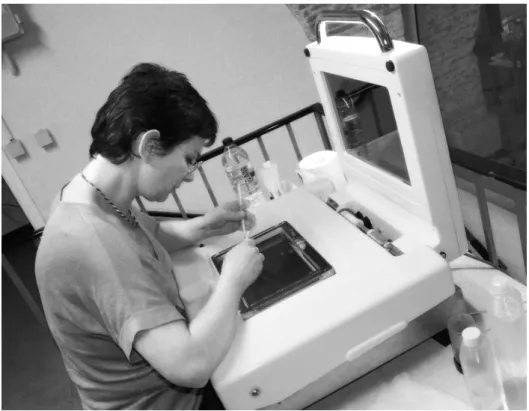
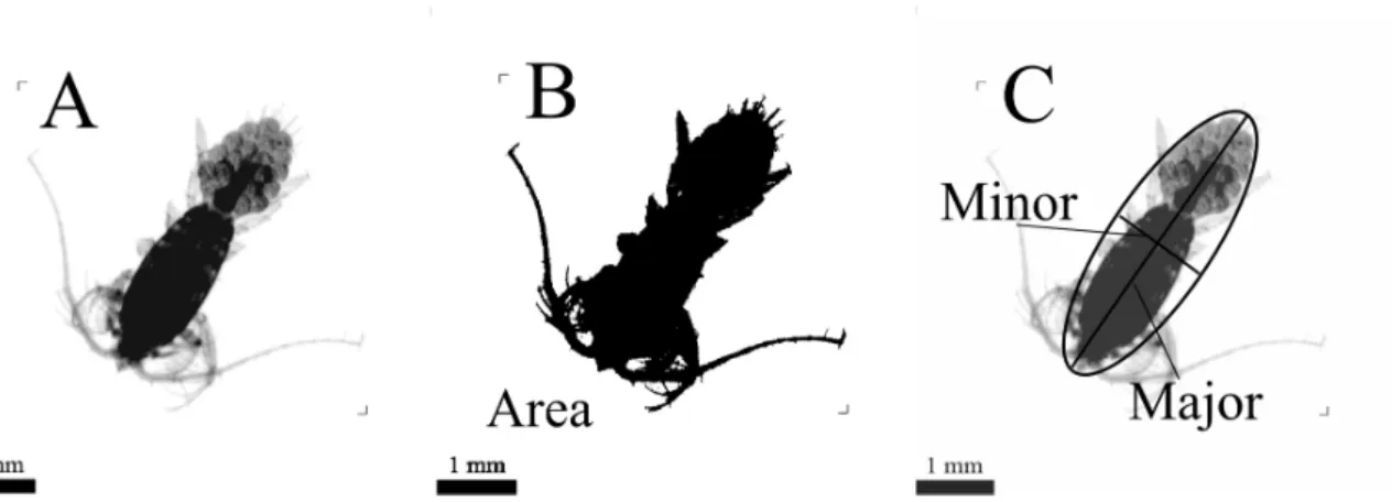
Carval. (B) picture of the NO Vellele and the WP2 net being operated by Mickaël Cayol and (C) the WP2 net underwater. Copyright Christophe Mocquet for A and B, and David Luquet for C. . . 25 I.4 Picture of the ZooScan model 2006 being operated by Corinne Desnos. . . 27 I.5 Image analysis on objects made with ZooProcess. (A), Raw image of a copepod
fe-male with eggs. (B), same object in black and white with a threshold of 243 for the computation of the area and (C), computation of minor and major axes of the best fitting ellipse. . . 28
II.1 Average validated size spectrum of the 22 samples used with the part represented by detritus, touching objects, crustaceans and other zooplankton (A). And (B), percent-age of these categories per size class. . . 48 II.2 Comparison of average size spectra measured during year 2003 with WP2 and
Ré-gent nets from visually validated samples. The size measure used is the elliptical biovolume. In (A), abundance size spectra and a linear curve with a slope of -2 are presented. (B) presents biovolume spectra and linear curve with a slope of -1. In (A) and (B) all zooplankton is presented. (C) shows the abundance size spectra and (D) the biovolume size spectra of the two nets for crustaceans only. The arrows point to particular values explained in the text. . . 51
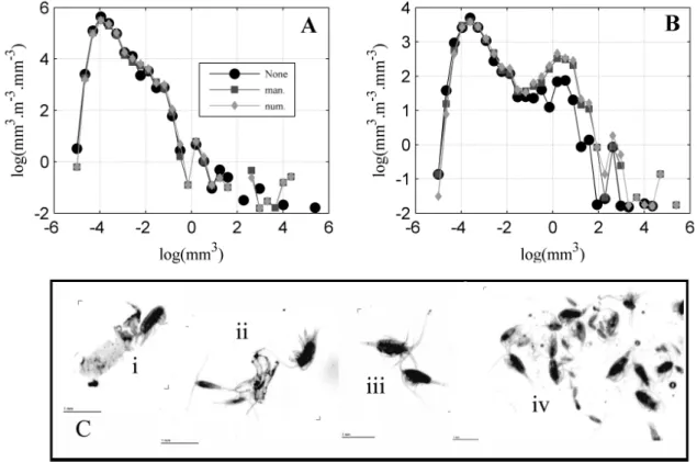
during 20 minutes (man.) and finally with a further numerical separation (num.). (A) experience one and (B) experience two. (C) examples of images with TO. . . 52 II.4 Comparison of predicted and validated recognition of crustaceans for total abundance
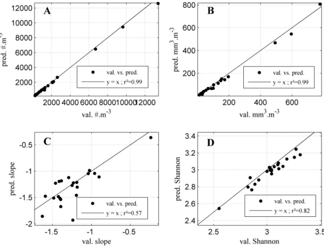
(A), total biovolume (B), slope of the linear regression (C) and Shannon entropy index (D) for the two years (2003 and 2006) which have been visually validated. . . 56 II.5 Four seasons (A: winter, B: spring, C: summer and D: autumn) of validated
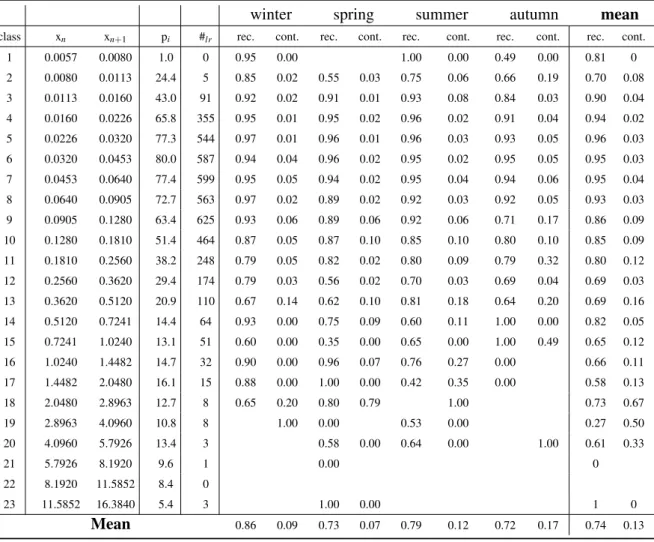
crus-taceans spectrum (white circle, Val. crust.), predicted cruscrus-taceans spectrum (black line, Pred. crust.) and from dark grey to light grey the composition of predicted crustaceans spectrum, which is respectively composed of crustaceans (Crust.), other zooplankters (Other zoo.), detritus (Det.) and touching objects (TO). In each figure is indicated the percentage of each of these groups inside the predicted crustaceans spectrum. The percentage of crustaceans is the value (1-contamination). . . 58 II.6 Confidence size range of the crustaceans spectrum (white) according to the mode (1:
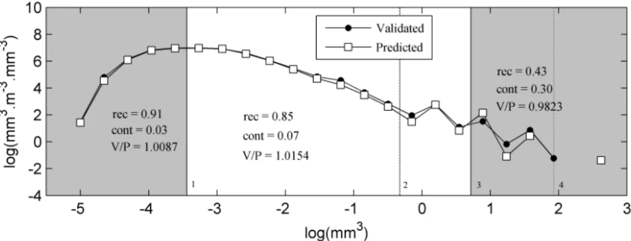
0.032 mm3) and the automatic classification minimum efficiency (3: 2.048 mm3). The more rigorous limit of the automatic classification efficiency (2: 0.724 mm3) and the crossing point of the WP2 and Régent nets zooplankton size spectra (4: 6.9 mm3) are also displayed. Recall (rec.), contamination (cont.) and the Validated/predicted (V/P) values are shown for three part of the spectrum. . . 59 II.7 Impact of spherical vs. elliptical biovolume measurements on the shape and
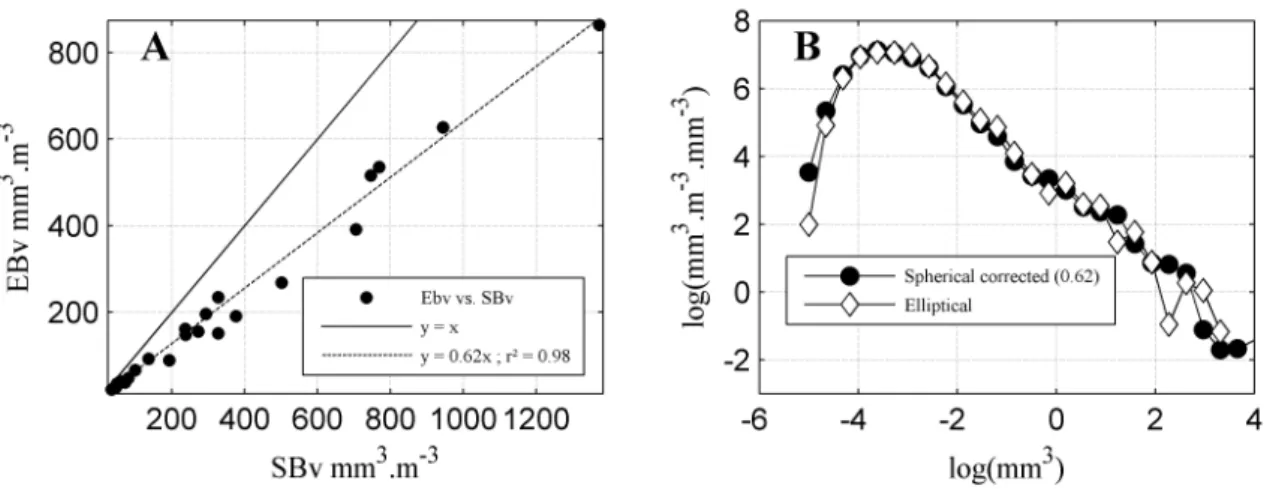
param-eters extracted from “N-BSS” of crustaceans. (A) total biovolume with a linear ad-justment y=0.62x, r2=0.98. (B) average “N-BSS” calculated with an elliptical bio-volume and “N-BSS” calculated with a spherical biobio-volume but corrected with the conversion factor 0.62 only (i.e., conversion to “N-NSS”, decrease of the nominal size by 0.62, then re-conversion to “N-BSS” using the new nominal size biovolume). 60 II.8 Comparison EBv vs. biomass (in µg m−3calculated from relationships of
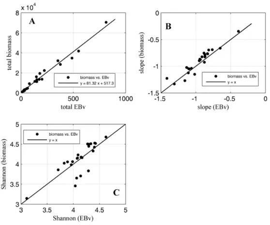
Hernández-León & Montero(2006) andLehette & Hernández-León(2009). (A) shows the rela-tionship between the total EBv and the total biomass of the zooplankton community, (B) shows the relationship between the slopes calculated from N-BbiovolumeSS and
N-BbiomassSS and (C) the relationship between Shannon index calculated from both
spectra. . . 63
III.1 Example of thumbnails directly issued from the ZooScan / ZooProcess of the ten identified zooplankton taxonomic groups. All thumbnails have the same scale (bottom right corner) except the small copepods which have their own scale on top left. . . . 71 III.2 De-noising of the zooplankton total abundance time series. Raw values are black dots
and the de-noised time series in shown in red. The de-noising was made using the Matlab functions “ddencmp” and “wdencmp” of the wavelet toolbox. . . 74
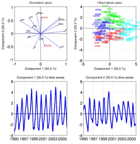
PC. In the space of observations (B), blue is for winter months (months 1,2 and 3), green is for spring months (4,5,6), cyan for summer months (7,8,9) and red for autumn (10, 11, 12). . . 75 III.4 PCA made on monthly values of environmental parameters. (A) represent the space
of descriptors, (B) the space of observations, (C) the time series of the first PC, and (D) of the second PC. In the space of observations (B), blue is for winter months (months 1,2 and 3), green is for spring months (4,5,6), cyan for summer months (7,8,9) and red for autumn (10, 11, 12). The two first PC of the zooplankton (fig. III.3) were added as external variables and are shown in red. . . 76 III.5 PCA made on annual values of zooplankton. (A) represent the space of descriptors,
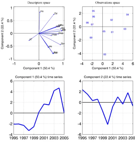
(B) the space of observations, (C) the time series of the first PC, and (D) of the second PC. . . 77 III.6 PCA made on annual values of environmental parameters. (A) represent the space of
descriptors, (B) the space of observations, (C) the time series of the first PC, and (D) of the second PC. For hydrological (“wT”, “wS” and “wD”) and meteorological parameters (“T”, “P”, “I”), annual means of each season were taken, the number correspond to the season, “1” is for months 1,2 and 3, “2” for months 4,5 and 6 until “4”. The two first PC of the zooplankton (fig.III.5) were added as external variables and are shown in red. . . 78 III.7 Detection of significant regime shifts in the two first PC of zooplankton and
environ-ment monthly values (section III.3.1.1 and fig.III.3CD,III.4CD) computed using the STARS methods ofRodionov(2004;2006). PC are shown in black were regimes are shown in magenta. Any step in the magenta curves indicate a significant regime shift. Parameters of the STARS method were a cut-off length of 2 years, a significant level p at 0.1, and the Huber weight at 1. . . 80 III.8 Objects classified with the modified Hausdorff distance. Monthly averaged and
lin-earized crustaceans N-BSS were taken. A log-transformation was then made to bal-ance the effect of small and large size classes. Each year is considered as a single object. For the computation of the Hausdorff distance a normalisation of each axis is made to make them varying from 0 to 1. More information on the computation of the modified Hausdorff distance is in sectionI.3.3.2. . . 81 III.9 Classification of objects of fig.III.8according to the modified Hausdorff distance —
the dendrogram was made using UPGMA linkage. . . 82
independent parameters were discarded (see text), it is shown by light blue in the up-per part of the matrix. black indicate a significant correlation <0.01 and grey <0.05. When correlations are opposite a white “-” is added. e.g. the Zooplankton total abun-dance anomalies (first line) are significantly correlated to zooplankton total biovol-ume and small copepods anomalies (p<0.01) and to crustaceans mean size (but op-posed), decapods larvæ, other crustaceans, spring temperature, spring irradiation and summer irradiation (p<0.05). A correction for multiple comparison was runned (see text), correlations significant (p <0.05) after this correction are in red circles (only three). Yellow circles are from the same procedure but with p <0.3, for indication only. 83 III.11Dynamics of total zooplankton biovolume (in mm3m−3) and abundance (in ind. m−3)
from 1995 to 2005. (A) annual anomalies of total biovolume; (B) annual anomalies of total abundance; (C) monthly values of total biovolume; (D) monthly values of total abundance. Black dots represents months with no values, they were then not used for analysis, anomalies computed on years with missing months must be taken with precaution. . . 86 III.12Cumulative sum of annual anomalies of the ten identified taxonomic groups: (A)
co for small copepods, Co for large copepods, de for decapods larvæ, cr for other crustaceans; (B) ch for chaetognaths, ap for appendicularians, pt for pteropods; (C) th for thaliaceans, ge for gelatinous predators, ot for other zooplankton. Small copepods account only for individuals between 0.032 and 0.724 mm3whereas the other groups account for individuals larger than 0.724 mm3. The cumulative sum method was first used in ecology byIbañez et al.(1993), a negative slope means a negative anomaly and vice-versa. . . 87 III.13Dynamics of crustaceans N-BSS indicators. A, B, C show the annual anomalies,
where D, E and F show the monthly values. A and D are the log-linear value of the slope, B and E are Shannon index and C and F are the determination coefficient R2 between the measured spectra and the log-linear fitting. Black dots represents months with no values, they were then not used for analysis, anomalies computed on years with missing months must be taken with precaution. . . 89 III.14Dynamics of nitrates (NO3) in µmol L−1 and chlorophyll-a in µg L−1. (A) annual
anomalies of NO3; (B) annual anomalies of chlorophyll-a; (C) monthly values of
NO3; (D) monthly values of chlorophyll-a. Black dots represents months with no
val-ues, they were then not used for analysis, anomalies computed on years with missing months must be taken with precaution. . . 90
nual anomalies of phosphates; (B) annual anomalies of silicates; (C) monthly values of phosphates; (D) monthly values of silicates. Black dots represents months with no values, they were then not used for analysis, anomalies computed on years with missing months must be taken with precaution. . . 91 III.16Dynamics of Suspended particles from 2.9 to 92.8 µm ESD calculated with the
Coul-ter CounCoul-ter. A, B, C show the annual anomalies, where D, E and F show the monthly values. A and D are the total abundance of particles in # m−3, B and E are the total biovolume of particles in mm3 m−3 and C and F are the log-linear slope of the N-BbiovolumeSS. Black dots represents months with no values, they were then not used
for analysis, anomalies computed on years with missing months must be taken with precaution. . . 93 III.17Annual anomalies of hydrological characteristics of the water column (averaged from
10 to 40 m) during the winter period, i.e., from the 4thto the 17thweeks which showed the maximum values of sea water surface density (unpresented data). Anomalies of (A) density (in kg m−3), (B) sea temperature (in ◦C) and (C) salinity (in psu). . . 94 III.18Anomalies of temperature of the water column (averaged from 20 to 80 m) for Point
B and DYFAMED stations in ◦C. (A) winter, January to March, (B) spring, April to June, (D) summer, July to September, (E) autumn, October to December and (C) all year. The Spearman rsand p are shown on each subfigures. . . 95
III.19Anomalies of salinity of the water column (averaged from 20 to 80 m) for Point B and DYFAMED stations in ◦C. (A) winter, January to March, (B) spring, April to June, (D) summer, July to September, (E) autumn, October to December and (C) all year. The Spearman rsand p are shown on each subfigures. . . 96
III.20Anomalies of density of the water column (averaged from 20 to 80 m) for Point B and DYFAMED stations in ◦C. (A) winter, January to March, (B) spring, April to June, (D) summer, July to September, (E) autumn, October to December and (C) all year. The Spearman rsand p are shown on each subfigures. . . 97
III.21Annual anomalies of climatic variables measured at the Sémaphore station (see fig. I.2): air temperature in ◦C (A and D), precipitation in mm d−1 (B and E) and solar irradiance in J cm−2d−1 (C and F). A, B and C report anomalies from autumn and winter months, i.e., from November of the previous year to March of the current year. And D, E and F report anomalies from spring and summer months, i.e., from April to August of the current year. . . 98 III.22Proposed general scheme of Ligurian Sea ecosystems dynamics, see sectionIII.4.3
for details. The legend of line and boxes is at the bottom of the scheme (Int. is for intermediate). (*) the quantity of previous year zooplankton cannot be verified, how-ever from Garcia-Comas et al. (Submitted) the beginning of the ’90s were low in zooplankton. . . 106
Arctic Oscillation, AMO for Atlantic Multidecadal Oscillation, NHT for Northern Hemisphere Temperature and ENSO for El-Niño Southern Oscillation. The winter value of the NAO was taken whereas annual means were taken for other indicators. . 109 III.24Correlations between main climate indicators and variables of the Ligurian
ecosys-tems previously highlighted from 1960 to 2008, i.e., “air T win” for air temperature in winter, “prec win” for winter precipitations, “Irr s/s” for spring / summer solar irradi-ation, “Dens win” for winter density of sea water, “Sal win” for winter salinity, “sea T win” for sea water temperature in winter and “zoo PC1” for the first PC on annual values of zooplankton (only from 1995 to 2005). Correlations were corrected using a FDR methods for multiples correlations. Only significant correlations at p<0.05 after the correction are shown, here with a black box. a white “–” in the box indicates an opposite correlation. . . 111
IV.1 Conceptual scheme of the size-based model at the population scale. see text for details.122 IV.2 Conceptual scheme of the physiological modeling at the individual scale. This
repre-sents the three possible directions of food that is ingested: the unassimilated part goes to detritus, and the assimilated part goes to growth (Soma) or reproduction (Germen). see text for details. . . 124 IV.3 Predator/prey affinity coefficient pzwith ρ=4 and σ=2 taken as example values to
illustrate the general shape of pz. . . 133
IV.4 Example of the shape of the grazing affinity coefficient pp. . . 133
IV.5 Example of the food effectively ingested vs. available food. . . 135 IV.6 Value of ppand µext with average parameters. . . 140
IV.7 Sentivity of derived parameters and equilibrium on variation in ka, the assimilation
coefficient. . . 141 IV.8 Sentivity of derived parameters and equilibrium on variation in kc, the proportion of
assimilated food allocated to growth. . . 141 IV.9 Sentivity of derived parameters and equilibrium on variation in ρ, the mean
preda-tor/prey size ratio. . . 142 IV.10 Sentivity of derived parameters and equilibrium on variation in σ , the variance of the
predator/prey size ratio. . . 142 IV.11 Sentivity of derived parameters and equilibrium on variation in βd, the exponent of
the digestion rate D(x). . . 143 IV.12 Sentivity of derived parameters and equilibrium on variation in ε, the maximum
frac-tion of ingested food at equilibrium. . . 143 IV.13 Sentivity of derived parameters and equilibrium on variation in T , the time to growth
from the minimum size x0to the maximum size x1at equilibrium, T is in days. . . . 144
the second is the total biovolume of zooplankton in mm3.m−3, the third one is the slopes of the N-BSS and the third is the N-BSS in log(mm3m−3mm−3). For the last three columns it is for size from x0to x1. The different scenarii are: (A) constant and
low, (B) constant and high , (C) Short and high peak, (D) long and lower peak, (E) two short and identical peaks and (F) one high peak followed by a smaller one. . . . 146 IV.15 Data used to compute the phytoplankton growth in the two scenarii (1: years 1996,
1997 and 1998, 2: years 2001, 2003, 2004 and 2005). (A) is the water temperature, (B) the nitrates, (C) the surface irradiation and (D) the irradiation in water computed with eq.IV.41. A, B and D are depth integrated values from surface to 75 m depth. . 150 IV.16 Phytoplankton biovolume (A) and growth (B) in the two scenarii (1: years 1996, 1997
and 1998, 2: years 2001, 2003, 2004 and 2005). A and B are depth integrated values from surface to 75 m depth. . . 151 IV.17 Crustaceans biovolume (A) and slope (B) in the two scenarii (1: years 1996, 1997 and
1998, 2: years 2001, 2003, 2004 and 2005). C and D represent the observed spectrum for the two scenarii. . . 152 IV.18 Comparison of observations and model outputs for the first scenario with default
val-ues of parameters, i.e., ka=0.4, kc=0.7, ρ =3.5, σ =2, βd =0.75, ε =0.75 and
T =360. . . 154 IV.19 Comparison of observations and model outputs for the second scenario with default
values of parameters, i.e., ka=0.4, kc=0.7, ρ=3.5, σ =2, βd=0.75, ε =0.75
and T =360. . . 155 IV.20 Comparison of observations and model outputs for the first scenario with a
prelim-inary optimization on parameters which gave ka=0.4, kc =0.7, ρ =3.5, σ =2,
βd =0.75, ε=0.3 and T =1080. . . 156
IV.21 Comparison of observations and model outputs for the second scenario with a pre-liminary optimization on parameters which gave ka=0.4, kc=0.7, ρ=3.5, σ =2,
βd =0.75, ε=0.3 and T =1080. . . 157
IV.22 Value of pp and µext with a preliminary optimization on parameters (ka=0.4, kc =
0.7, ρ=3.5, σ=2, βd=0.75, ε=0.3 and T =1080). . . 158
V.1 General scheme of biases and solutions in the measurement of zooplankton size spec-tra. See text for explanation on numbers. . . 166 V.2 General scheme of links between climate, hydrology and biology in the Ligurian
Sea from present findings. NAO is for North Atlantic Oscillation, NHT for Northern Hemisphere Temperature and AMO for Atlantic Multidecadal Oscillation. . . 173
together with the application of the STARS methods to detect shifts (see chapterIII). The second graph shows annual anomalies of copepods abundances. . . 178 V.4 Same as in fig.V.3but on log(abundances +1). . . 179
A.1 Raw zoological, biological, hydrological and meteorological data from Point B and Sémaphore stations used in this chapter. For all parameters the complete raw time series is shown together with a boxplot made on month values. Zooplankton data come from WP2 sampling from 60 m depth to surface. Biological and suspended particles come from NISKIN bottles at 6 different depths, shown values are depth averaged. Hydrological data come from CTD casts, average value from 10 to 40 m were taken. Meteorological data come from daily measurements, the average weekly values were taken. Red curves present the de-noised time series using the matlab func-tion “ddencmp” and “wdencmp”. Finally, the magenta curves represent the results of shifts detection following the STARS method ofRodionov(2004;2006), any step in these curves indicates a significant change (at the threshold of 0.1) in the mean with the cut-off length being set to two years. . . 189 A.1 suite. . . 190 A.1 suite. . . 191 A.1 suite. . . 192 A.1 suite. . . 193
B.1 Number of weeks sampled per month, from 0 to 5, for the four time series: JB 1, JB 2, WP2 1, WP2 2. . . 198 B.2 Number of tows per month, from 0 to 35, for the four time series: JB 1, JB 2, WP2 1,
WP2 2. . . 199 B.3 Copepods abundances of all time series from 1966 to 2010 shown together — it is
displayed on two graphs for more clarity. See text for significance of JB 1, JB 2, WP2 1 and WP2 2. The time series analyzed in chapterIIIis WP2 1. . . 200
II.1 Results of the two experiments made to assess the impact of Touching Objects (TO) on the observed spectrum. The two samples were first scanned without any separation (none), then with a manual separation (man.) on the scanning tray, and finally with the further use of a numerical (num.) separation tool implemented in ZooProcess. The abundance (Ab, # m−3), percentage of the abundance (% Ab), biovolume (Vol, mm3 m−3) and percentage of biovolume (% Vol) is presented for three categories, i.e., non biologic particles (detritus and fibers), touching objects and zooplankton. . . 54 II.2 Results of the confusion matrix based on the validation set. The number of objects in
the learning set (#lr), the relative abundance in the field (piin %) and recall (Rec.) and
contaminations (Cont.) rates are presented for each category and also for the synthetic categories all zooplankton (All zoo.) and all crustaceans. . . 55 II.3 Recall (rec.) and Contamination (cont.) for crustaceans related to the size class and the
season issued from fig.II.5. For each size class the lower (xn) and upper (xn+1) limits,
the relative abundance in the field (piin %), the number of objects in the learning set
(#lr) and recall (rec.) and contamination (cont.) for the four seasons and the mean are
presented. . . 57 II.4 Average Minor:Major ratio (±std), slope (b) of the regression EBv=b· SBv, r2of the
regression and number of individuals used for the regression (N) for the 11 zooplank-ton categories. . . 60 II.5 Relations used to computed the dry weight (in µg) from the area (in mm3) measured
by image analysis. the relation “Copepods” was used for categories copepods and nauplii — “Chaetognaths” was used for chaetognaths — “Other crustaceans” was used for decapods, cladocerans, Penilia avirostris and other crustaceans — “Gelati-nous” was used for gelatinous — “Other” was used for all other categories. +is for relations fromHernández-León & Montero(2006) andois for relations fromLehette & Hernández-León(2009). . . 61
size range (for indication only), representative species or groups and dominant diet considered in this work. The category “Copepods (small)” comes from copepods au-tomatically sorted from 0.032 to 0.724 mm3and the percentage given applies on
zoo-plankton of this size range only. The large zoozoo-plankton (i.e., >0.724 mm3) represent 1.8 and 31.5 % of total zooplankton abundance and apparent biovolume respectively. 73 III.2 Timing (week number) of starting and maximum of seasonal variables, i.e., the
ni-trates (NO3), the chlorophyll-a (chl-a), the zooplankton total abundance (Zoo.) and
the stratification of the water column (Strat.). . . 85
IV.1 Complete list of variables and parameters used in the zooplankton continuous size-based model. The currency is basically the energy and a proportional relation was assumed with biomass and biovolume. In this table we will use “mm3” for units to be consistent with the measured made on the ecosystem. . . . indicates parameters that have to be set (mean and range values are then given) and “*” indicates parameters that are calculated within the model to ensure an allometric equilibrium, see text for explanation. . . 125 IV.2 Parameters default values (mean) and range of variation (min to max) determined
from literature. See sectionIV.2.4. . . 139 IV.3 Units and values used for computing the irradiance at depth z. . . 148 IV.4 Kwater(z). . . 149
IV.5 Units and values used for computing phytoplankton growth µ at depth z . . . 150
I
I.1 ZOOPLANKTON CHANGES IN THEMEDITERRANEANSEA . . . 4
I.2 SIZE-BASED ANALYSIS AND MODELING OF THE ZOOPLANKTON . 7
I.2.1 Meaning of size for zooplankton . . . 8 I.2.2 Measuring the size . . . 11 I.2.3 Size-based theory and models . . . 12 I.2.4 Incorporating size in models . . . 18 I.3 METHODS. . . 23 I.3.1 Localization of the sampling site . . . 23 I.3.2 Imaging procedure . . . 26 I.3.2.1 Samples used . . . 26 I.3.2.2 Imaging procedure . . . 26 I.3.2.3 Automatic classification of objects . . . 28 I.3.2.4 Size-spectra computation . . . 30 I.3.3 Statistical analyses . . . 31 I.3.3.1 Identifying regime shifts . . . 32 I.3.3.2 Computing distances between size spectra . . . 36 I.4 ORGANIZATION OF THE THESIS. . . 38
T
HEmarine realm and its inhabitants are a fantastic area of discovery and, besides their beauty, play a major role in the global earth system. The living part of the water column iscom-posed — apart from marine mammals and adult fishes — of plankton (from the greek planktos, i.e.
drifter, wanderer). Then, plankton represent the most part of the sea life. A distinction is made
be-tween its different components, the viroplankton, the bacterioplankton, the nano-, micro- and
macro-phytoplankton, the micro-, meso- and macro-zooplankton. This thesis is focused on
mesozooplank-ton and their links with other plankmesozooplank-ton components as well as with the chemical and physical
en-vironment. The mesozooplankton comprises all animals living in the water column from about 200
µ m length to few mm and belonging to various taxonomic groups such as crustaceans, cnidarians,
ctenophors, gastropods, chaetognaths, annelids, tunicates and fish larvæ. The most important group,
in terms of abundance, being the crustaceans and especially copepods, (see Mauchline 1998, for
a review of marine calanoid copepods) which play major roles in marine food webs and
biogeo-chemical cycles (e.g.,Smetacek 1985,Banse 1995,Verity & Smetacek 1996,Mackas & Beaugrand
2010). Copepods transfer energy from phytoplankton to higher trophic levels such as fish and large
gelatinous predators. More than 80 years ago, Charles Elton said, “It will be shown that the
peri-odic fluctuations in the number of animals must be due to climatic variation” (Elton 1924). With
the growing concern on climate change, tracing and understanding the impact of climate onto the
dynamics of marine animals and ecosystems has become a major issue in biological oceanography
(e.g.,Aebischer et al. 1990,Fromentin & Planque 1996,Beaugrand & Ibañez 2002,Drinkwater et al.
2003,Mysterud et al. 2003,Stenseth & Mysterud 2003,Richardson 2008,Kirby & Beaugrand 2009,
response to ecosystem variability, their non-exploitation for commercial purposes and their
amplifi-cation of subtle changes through non-linear processes, zooplankton have been pointed out as good
sentinels of climate changes (Taylor et al. 2002,Perry et al. 2004,Hays et al. 2005).
I.1
Z
OOPLANKTON CHANGES IN THEM
EDITERRANEANS
EAThe Mediterranean Sea is the largest quasi-enclosed sea on the Earth connected to the Atlantic Ocean
through the Gibraltar strait that is only 14 km width. The Mediterranean has a total area of nearly
2.5 × 10⁶km2 (52000 km2 for the Ligurian Sea) and 46000 km of coasts which makes the coast /
surface ratio particularly high (Meybeck et al. 2007) and highlights the importance of the land-sea
interface and of the impact of human activities. The Mediterranean geology and particular climatic
features allow for a rich and complex physical dynamics with unique thermohaline features, distinct
multilayer circulation, topographic gyres, meso- and submeso-scale activity (Zavatarelli & Mellor
1995, Millot 1999, Pinardi & Masetti 2000). A nice review of the Mediterranean Sea, focused on
plankton and factors affecting it had been recently published bySiokou-Frangou et al.(2010).
The trophic state of the Mediterranean Sea ranks from oligotrophic to ultra-oligotrophic, with
a clear decrease from the western to the eastern basin and from the north to the south (D’Ortenzio
& d’Alcala 2009). According to phytoplankton biomass, estimated as chlorophyll-a from remote
sensing, different oceanic provinces were defined (D’Ortenzio & d’Alcala 2009). The North Western
(NW) region shows patterns similar to temperate areas, unique in the Mediterranean Sea, consisting
in a late winter / spring phytoplankton bloom lasting as long as three months with a biomass increase
up to 6 times the background value (Levy et al. 1998) and a frequent autumn bloom. The coastal and
central parts of the NW Mediterranean belong to another province characterized by an intermittency
of temperate and subtropical modes, i.e. more oligotrophic and less marked spring bloom (D’Ortenzio
river runoff, atmospheric fertilization, or continental shelf dynamic: mainly Alboran Sea, Adriatic
Sea, south of Tunisia, Catalan front, Gulf of Lion. This applies however only to autotrophs. The low
standing stocks of them are generally justified by “bottom-up” constraints. It was however shown that
purely heterotrophic processes may produce a rapid transfer to higher levels, even in less productive
area, suggesting possible strong “top-down” effects (Thingstad et al. 2005, for ciliates and bacteria).
Therefore, two possible views emerged, the low abundance of autotrophs being the result of low
nutrients availability or being the result of an effective control by grazers, with a trophic cascade
propagating up to top predators (Siokou-Frangou et al. 2010). The latter view is supported by the
observation that standing stocks of top predators (fishes) are higher than would have been expected
on the basis of chlorophyll-a and nutrient stocks (Fiorentini et al. 1997). “Bottom-up” and
“top-down” controls can both affect the structure of food webs. This is at the origin of the “Mediterranean
paradox” (Sournia 1973,Estrada 1996,Siokou-Frangou et al. 2010), which moderates the view of the
Mediterranean Sea as an oligo- to ultra- oligotrophic Sea.
Some trends toward oligotrophy have recently been observed in marine basins (Molinero et al.
2005;2008,Barale et al. 2008,Mozetic et al. 2010,Steinacher et al. 2010) suggesting climate driven
changes in the trophic states of ecosystems. Regime shifts, i.e., abrupt changes in the state of a system,
were reported with effects on zooplankton communities. For example, in the Atlantic ocean, a regime
shift from cold to warm biotopes, with a turning point in 1987, has been described and related to
the North Atlantic Oscillation (NAO,Hurrell & Deser 2010) and surface temperature anomalies in
the Northern Hemisphere (NHT,Reid et al. 2001;2003, Beaugrand 2004,Beaugrand et al. 2008).
Regarding Mediterranean plankton, very few studies on long-term variations have been conducted,
due to the paucity of long-term time series (Mazzocchi et al. 2007). Recently, it has been highlighted
the appearance of regime shifts — toward more oligotrophic states — with their turning points in 1987
with changes in the Atlantic Ocean and the Baltic and Black seas (Conversi et al. 2010). The authors
pointed out the positive trend of surface temperature in the northern hemisphere as the main forcing
for the concomitant changes in such far and different regions. In the Balearic Sea (Fernàndes de
Puelles et al. 2007, studied period: 1994-2003), a decrease of zooplankton abundance was observed
from 1995 to 1998 with a recovery of all groups from 2000. Such an inter-annual variability was
linked to the NAO forcing. In its positive phase, the NAO drives colder temperature during winter
months enhancing the southward spread of rich northern Mediterranean waters in the Balearic Sea
(Fernàndes de Puelles et al. 2007,Fernàndes de Puelles & Molinero 2008). From a comparative study
of six zooplankton time series in the Mediterranean Sea, synchronous cooling and warming phases
was observed in Trieste, Naples and Villefranche-sur-Mer, with, again, a main turning point in 1987
associated to a decrease of zooplankton abundances (Berline et al. accepted) — yet, no significant
links with large scale climate indicators such as the NAO were found. Other studies in the Ligurian
Sea, based on a long time series (1963-1993) in the bay of Villefranche-sur-mer, have also suggested
that the pelagic ecosystem was heading toward a more regenerated system dominated by jellyfish
in the early ’90s (Molinero et al. 2008). A more recent study from the same time series extended
until 2003 revealed that the zooplankton and mainly copepods recovered their initial concentrations
after 2000 suggesting a quasi decadal cycle (Garcia-Comas et al. Submitted). Such a recovery from
ca. 2000 was also observed by Berline et al.(accepted) in Villefranche-sur-Mer, by Fernàndes de
Puelles et al. (2007) in the Balearic Sea. In Naples the recovery occured in 2004 (Berline et al.
accepted). The higher abundance of zooplankton were correlated to dry and cold winter resulting
in high winter mixing. Dry and cold winters lead to a rise in surface density increasing the winter
convection and, as suggested by the authors, enhancing nutrients replenishment and strengthening the
spring bloom. The positive effect of dry winters was observed on the entire zooplankton community
initiated by the intensity of the winter convection is also supported by observations in the southern
and central Ligurian Sea (Goffart et al. 2002,Nezlin et al. 2004,Marty & Chiavérini 2010), yet with
no consideration of zooplankton.
The Mediterranean appears then as a complex system with a strong heterogeneity at the basin
scale, but also at the mesoscale. To understand the zooplankton dynamics and how it is affected by
environmental and climatic factors different approaches can be followed. A very promising approach
is based on the size distribution of zooplankton communities and will be presented hereafter.
I.2
S
IZE-
BASED ANALYSIS AND MODELING OF THE ZOOPLANKTONCommon models utilized for investigating marine ecosystems are partitioned in different boxes
(nu-trients, phytoplankton, zooplankton, detritus) each of them being defined by an input and an output of
matter. To make this kind of models more realistic, authors generally try to add more and more boxes
— the zooplankton box becoming for example: copepods and appendicularians. Each box is defined
by a gain and a loss of matter at each time step — generally computed by one equation (Fasham
et al. 1990). But these models drive to a multiplication of links and parameters (Moloney & Field
1991) that are not available and consequently are generally arbitrary in such models. An observation
allows to avoid this problem: organisms belonging to different taxonomic categories can be grouped
according to their size. This means that, for example, a fish larvæ is closer to an adult copepod than to
an adult fish of the same species (Bertalanffy 1957,Peters & Wassenberg 1983). Hence, it becomes
possible to simplify zooplankton by a measurement of their biomass by size, the so-called
biomass-size spectra (N-BSS,Sheldon et al. 1972,Platt & Denman 1977). This is “A simple, understandable,
first-order approximation to the dynamics of the system as a whole” (Heath 1995). A mathematical
framework has emerged from this measurement, used to calculate some parameters of the ecosystem
& Kerr 1972) and several other parameters (Edvardsen et al. 2002,Zhou 2006). This measurement
starts to be commonly used in ecosystem models (Moloney & Field 1991,Moloney et al. 1991,Gin
et al. 1998,Armstrong 1999,Benoît & Rochet 2004,Baird & Suthers 2007,De Eyto & Irvine 2007,
Maury et al. 2007a;b,Stock et al. 2008,Zhou et al. 2010). A review of models for zooplankton
stud-ies can be found in Carlotti & Poggiale(2010). The following sections will present the importance
of size for the physiology and the interactions within zooplankton. Theoretical and modeling studies
based on the size spectrum will also be shown.
I.2.1 Meaning of size for zooplankton
It is now well known that physiological rates scale with size more than with taxonomy (Bertalanffy
1957,Fenchel 1974,Peters & Wassenberg 1983,West et al. 2003,Glazier 2005,Hendriks 2007). It
is also commonly accepted that the scaling has the form (Brown et al. 2004)
Y = α xβ (I.1)
where Y is the response (for example metabolic rate), x the size, α a normalization constant and β
the scaling exponent. If β equals 1, the relation is isometric, otherwise it is allometric. This relation is
linear but this is not always the case as it can also be non-linear. There are different kinds of possible
scaling in nature. Glazier (2005), in the continuum of Bertalanffy (1957), separated four kinds of
relations. But for the sake of simplicity most of the works used the linear one (type I). This kind
of scaling (power-law) is considered to be universal (Stanley 1995).Marquet et al.(2005) reviewed
these power-laws in ecological systems.
Yet, this is not always the case in biology (e.g.,Chaui-Berlinck 2006,O’Connor et al. 2007), but
a large part of the scientific community went further by arguing that the exponent α of the relation is
always 3/4 (West et al. 2003,Brown et al. 2004). This 3/4 scaling is usually observed in allometric
nature as it can sometimes be very far from this value. Copepods, for example, show a mean scaling
exponent of 0.84 and, if we include all other pelagic species, this exponent rise to 0.94 (Glazier 2005).
This scaling is explained by the fractal geometry of organisms, while an euclidean geometry would
lead to a 2/3 scaling (Peters & Wassenberg 1983), also observed in nature (Glazier 2005). Yet,Brown
et al.(2004) proposed the “metabolic theory of ecology”, a size-based allometry with an exponent of
3/4 and a temperature normalization (i.e., e−E/kT). This is a simplification of the complex ensemble
of physiological processes but it may suffice to study high levels of organization like ecosystems.
Starting from the same type of relation, other authors gave more complex definitions of allometric
scaling that allowed for different values of the exponent (Demetrius 2006,Hendriks 2007,da Silva
et al. 2007).
Another way of explaining the relation between size and physiology emerged from the so-called
“Dynamic Energy Budget” theory (DEB,Kooijman 1986; 2001,Nisbet et al. 2000, van der Meer
2006, Sousa et al. 2006; 2008). In this theory, the 3/4 scaling was not assumed but found back
very easily. This global model of the physiology of organisms can have different parameters and
variables but the main mechanisms are the same for all living organisms (Kooijman 1986; 2001).
A fraction of the energy ingested is assimilated while the other part is directly rejected (feces). The
assimilation is then separated in two fractions: one for the soma and the other one for the gonads
and reproduction (plus maintenance costs). Between organisms of different species, parameters can
change, but between organisms of the same species the only differences occur in the state variables,
i.e., reserve and structural mass. Using DEB theory, a small organism invests relatively less energy in
somatic maintenance than a larger one, so a small organism has a metabolic rate lower than that of
a large organism of the same species. Metabolic rates are linear combinations of actual body length
(Nisbet et al. 2000). This theory seems to be a good approach to the physiology of individuals and has
been used byMaury et al.(2007a) to model the physiology of the consumers in an ecosystem model.
Size is also of great importance in the way organisms get in contact for processes such as
preda-tion, grazing, mating, swarming or aggregation (e.g.,Jackson 1990,Jackson & Burd 1998,Kiorboe
2001,Kriest & Evans 2000,Jackson & Kiorboe 2004,Stemmann et al. 2004a;b,Visser & Kiorboe
2006,Visser 2007). Encounter rates in marine environment were first studied on inert particles by
Jackson(1990) who proposed a model to calculate the probability of encounter of two particles
de-fined by their size based on different processes: the Brownian diffusion, the differential sedimentation
and the shear or turbulence. The Brownian diffusion is the intrinsic behavior of particles. The model
ofJackson et al.(1995) was used byBaird & Suthers(2007) to model encounter rates between living
organisms in a size-resolved pelagic ecosystem. In the perspective to resolve a global model by size,
models of encounter rates are useful because all kernels (processes by which encounters occur) are
related to the size of particles (living or not). Yet, for zooplankton, the behavior is far more
com-plex than a Brownian motion and is affected by many external factors (e.g.,Schmitt & Seuront 2001,
Schmitt et al. 2006,Vandromme et al. 2010) — this is why some studies have been undertaken to
de-scribe other processes. For example,Jackson & Kiorboe(2004) give a kernel formulation for finding
particles by zooplankton using a chemodetection of the chemical plume following particles in marine
environment — such formulation being also related to the size of both zooplankters and particles.
This can be added to other grazing behaviors defined byVisser(2001) like ambush, cruising or flux
feeding (also related to size). The last step is to define the encounter mechanisms and rates between
living zooplankton. An attempt was made byVisser & Kiorboe(2006) to define the encounter kernel
for two kinds of movement: ballistic and diffusive. The shift between these two motion behaviors
de-pends on the interaction scale compared to the movement scale. The variety of swimming behaviors