HAL Id: hal-03230940
https://hal.sorbonne-universite.fr/hal-03230940
Submitted on 20 May 2021HAL is a multi-disciplinary open access archive for the deposit and dissemination of sci-entific research documents, whether they are pub-lished or not. The documents may come from teaching and research institutions in France or abroad, or from public or private research centers.
L’archive ouverte pluridisciplinaire HAL, est destinée au dépôt et à la diffusion de documents scientifiques de niveau recherche, publiés ou non, émanant des établissements d’enseignement et de recherche français ou étrangers, des laboratoires publics ou privés.
Longitudinal Structural MRI in Neurologically Healthy
Adults
Sarah Gregory, Keith Lohse, Eileanoir Johnson, Blair Leavitt, Alexandra
Durr, Raymund A.C. Roos, Geraint Rees, Sarah Tabrizi, Rachael Scahill,
Michael Orth
To cite this version:
Sarah Gregory, Keith Lohse, Eileanoir Johnson, Blair Leavitt, Alexandra Durr, et al.. Longitudinal Structural MRI in Neurologically Healthy Adults. Journal of Magnetic Resonance Imaging, Wiley-Blackwell, 2020, 52 (5), pp.1385 - 1399. �10.1002/jmri.27203�. �hal-03230940�
Longitudinal Structural MRI in
Neurologically Healthy Adults
Sarah Gregory PhD,
1,2*
Keith R. Lohse PhD,
3,4Eileanoir B. Johnson PhD,
1Blair R. Leavitt MD,
5Alexandra Durr MD PhD,
6Raymund A.C. Roos MD PhD,
7Geraint Rees MD PhD,
2,8Sarah J. Tabrizi MD PhD,
1Rachael I. Scahill PhD,
1and
Michael Orth MD PhD
9,10Background: Structural brain MRI measures are frequently examined in both healthy and clinical groups, so an understand-ing of how these measures vary over time is desirable.
Purpose: To test the stability of structural brain MRI measures over time. Population: In all, 112 healthy volunteers across four sites.
Study Type: Retrospective analysis of prospectively acquired data.
Field Strength/Sequence: 3 T, magnetization prepared– rapid gradient echo, and single-shell diffusion sequence. Assessment: Diffusion, cortical thickness, and volume data from the sensorimotor network were assessed for stability over time across 3 years. Two sites used a Siemens MRI scanner, two sites a Philips scanner.
Statistical Tests: The stability of structural measures across timepoints was assessed using intraclass correlation coefficients (ICC) for absolute agreement, cutoff≥0.80, indicating high reliability. Mixed-factorial analysis of variance (ANOVA) was used to examine between-site and between-scanner type differences in individuals over time.
Results: All cortical thickness and gray matter volume measures in the sensorimotor network, plus all diffusivity measures (fractional anisotropy plus mean, axial and radial diffusivities) for primary and premotor cortices, primary somatosensory thalamic connections, and the cortico-spinal tract met ICC. The majority of measures differed significantly between scan-ners, with a trend for sites using Siemens scanners to produce larger values for connectivity, cortical thickness, and volume measures than sites using Philips scanners.
Data Conclusion: Levels of reliability over time for all tested structural MRI measures were generally high, indicating that any differences between measurements over time likely reflect underlying biological differences rather than inherent meth-odological variability.
Level of Evidence: 4. Technical Efficacy Stage: 1.
J. MAGN. RESON. IMAGING 2020;52:1385–1399.
B
RAIN MORPHOLOGY and anatomical connectivity are central to the in vivo characterization of biological mechanisms underlying neurodegeneration. Reliably measur-ing both structure and connectivity can provide informationregarding the nature of disease-related changes that occur across the course of disease progression. This can improve our understanding of the way in which pathology impacts not only structure, but also brain activity and behavior, while such
View this article online at wileyonlinelibrary.com. DOI: 10.1002/jmri.27203 Received Feb 25, 2020, Accepted for publication May 7, 2020.
*Address reprint requests to: S. G., Huntington’s Disease Centre, University College London, 2nd Floor, Russell Square House, 10-12 Russell Square, London WC1B 5EH, UK. E-mail: [email protected]
From the1Huntington’s Disease Research Centre, Institute of Neurology, University College London, London, UK;2Wellcome Centre for Human
Neuroimaging, Institute of Neurology, University College London, London, UK;3Department of Health, Kinesiology, and Recreation, University of Utah, Salt
Lake City, Utah, USA;4Department of Physical Therapy and Athletic Training, University of Utah, Salt Lake City, Utah, USA;5Centre for Molecular Medicine and
Therapeutics, Department of Medical Genetics, University of British Columbia, Vancouver, British Columbia, Canada;6APHP Department of Genetics,
Pitié-Salpêtrière University Hospital, and Institut du Cerveau et de la Moell épinière (ICM), Sorbonne Université, Paris, France;7Department of Neurology, Leiden
University Medical Centre, Leiden, The Netherlands;8Institute of Cognitive Neuroscience, University College London, London, UK;9Department of Neurology,
Ulm University Hospital, Ulm, Germany; and10Neurozentrum Siloah, Bern, Switzerland
Additional supporting information may be found in the online version of this article
This is an open access article under the terms of the Creative Commons Attribution License, which permits use, distribution and reproduction in any medium, provided the original work is properly cited.
changes can also act as valuable markers for both the timing and efficacy of therapeutic treatment at an exploratory level.
In thefield of neuroimaging, higher-resolution structural magnetic resonance imaging (MRI) is used to examine brain macrostructure including volume, cortical thickness, and sur-face area, while diffusion-weighted MRI is one method that interrogates the microstructural properties of white matter.1 Both techniques are employed to measure either region-specific or whole-brain structural changes across clinical groups, includ-ing those with neurodegenerative disease.2,3In particular, struc-tural MRI can be used to highlight and index morphological differences in regions of the brain associated with specific pathologies, as compared to healthy controls (or other disease-groups), and how these differences change over the course of a disease trajectory.4 There is very robust structural MRI evi-dence, for example, of striatal degeneration in the early stages of Huntington’s disease (HD)5,6 and in the medial temporal lobe in probable Alzheimer’s disease (AD),7,8 while structural
measures can inform clinical diagnosis and treatment decisions in disorders such as multiple sclerosis and dementia.9,10 Struc-tural MRI-derived measures of brain volume are currently included as secondary endpoints in clinical trials. However, while routinely used in research studies, due to the complexity of diffusion-weighted MRI acquisition and analysis, micro-structural measures have not yet been used in clinical trials.
Despite the clear utility of both structural and diffusion-weighted MRI, it is also important to consider that, as with any imaging technique, both noise and variations can be introduced at almost any stage. Rigorous protocol stan-dardization and staff training notwithstanding, potential sources of variation include local magneticfield inhomogenei-ties, experimenter bias, inherent issues within analysis pack-ages, and, importantly, differences between the individuals being scanned. All of these causes of variability are unrelated to the hypotheses that are being tested, but need to be con-sidered when interpreting data. Multisite studies are becom-ing more frequent and they customarily include several different scanner types and models, in addition to variation in site personnel. Hence, a sound understanding of the nature and subsequent prevention of intersite differences is increas-ingly important.
Promisingly, there is some evidence to suggest that both standard scalar diffusion tensor imaging (DTI) metrics includ-ing diffusivity and fractional anisotropy (a ratio of diffusivity perpendicular and parallel to the direction of the main underly-ingfiber) and volumetric measures are reproducible across sites and scanner types despite predictably greater between-site vari-ability.11-13 However, most investigations have tended to use imaging phantoms to assess MRI reproducibility or small groups of healthy controls over very short time intervals.11-13 While useful, this does not provide sufficient guidance for large multisite observational studies or clinical trials that examine participants over intervals of up to a year or longer.14,15It is
important to have a clear grasp of the reliability of structural measures in order to understand disease progression (or its modification by treatment) over substantial time intervals. This consideration is especially important in populations where brain structure is known to change over time (eg, in neurode-generative populations). Therefore, investigating reproducibility of imaging measures in healthy volunteers over longer time periods can help characterize variability over time due to mea-surement error or systematic biological change (eg, “healthy” age-related change). This, in turn, can help distinguish genuine effects related to pathology in disease populations. Accordingly, a recent study retrospectively examined the reliability of elec-trophysiological data in healthy individuals from the Track-On HD multisite longitudinal study over three annual timepoints using intraclass correlation coefficients (ICCs) and demon-strated that some measures met the criteria for high levels of stability, while others did not.16The study also identified lim-ited between-site differences.
Here we have similarly retrospectively investigated the reliability of structural and diffusion MRI-based metrics of volume, cortical thickness, and anatomical connectivity focus-ing on the sensorimotor network in a similar cohort of healthy individuals from TrackOn-HD.2,17 We aimed to characterize the effects of time, scanner type, and site on structural brain MRI measures.
Materials and Methods
Participants
Healthy control participants were recruited into the TrackOn-HD study at four study sites (London, Paris, Leiden, Vancouver).2,17For the present analyses, we used data from 112 participants (F = 67; mean age = 48 years ± SD: 11 years) who had complete DTI data for all three timepoints. Exclusion criteria included age below 18 or above 65 (unless previously in the Track-HD study), major psychiat-ric, neurological, or medical disorder or a history of severe head injury.17 The study was approved by the local Ethics Committees, and all participants gave written informed consent according to the Declaration of Helsinki. At visits one to three, individuals had an average age of 48.1 years (SD: 10.7), 49.4 years (SD: 10.5), and 51 years (SD: 10.3), respectively. Attrition rates were low. At visit two, retention of participants was 93% and at visit three 87%. Table 1 contains demographic information about participants bro-ken down by study site and scanner.
MRI Data Acquisition and Analysis
Data acquisition across sites was standardized as previously described.2,18In short, all site staff participated in a training session
and regular contact was maintained between sites and study coordi-nation throughout data collection. Prior to the start of the study, a human phantom was used at all sites to ensure identical settings and instructions. Throughout the study, data quality was monitored visu-ally by IXICO (UK; Contract Research Organization). In parallel, quality control (QC) software was applied to all scans within 3 work-ing days of acquisition. 3T MRI data were acquired on two different
scanner systems (Philips Achieva at Leiden, Netherlands, and Van-couver, British Columbia, Canada, and Siemens TIM Trio at London, UK, and Paris, France). T1-weighted image volumes were
acquired using a 3D magnetization prepared rapid gradient echo (MPRAGE) acquisition sequence with the following imaging param-eters: relaxation time (TR) =2200 msec (Siemens [S]) / 7.7 msec (Philips [P]), echo time (TE) = 2.2 msec (S) / 3.5 msec (P), flip angle (FA) = 10o(S)/8o(P),field of view (FOV) = 28 cm (S) / 24 cm (P), matrix size 256× 256(S)/224 × 224(P), 208(S)/164(P) sagittal slices with a slice thickness of 1.0 mm with no gap. Diffusion-weighted images were collected with 42 unique gradient directions (b = 1000 sec/mm2) on both scanner types plus eight images with no diffusion weighting (b = 0 sec/mm2) (S) and one image with no diffusion weighting (b = 0 second/mm2) (P). Acquisition parameters were TE = 88 msec, TR = 13,000 msec, and voxel size 2× 2 × 2 mm (S); TE = 56 msec and TR = 11 sec, and voxel size 1.96× 1.96 × 2.75 mm (P).
T1Processing
T1scans underwent visual QC upon data collection (performed by
S.G., E.J., R.S.) to check for incorrect parameters in the metadata and image artifacts such as motion artifacts. Scans were then bias-corrected to correct for inhomogeneity within the images using the N3 algorithm.19Images were segmented using FreeSurfer v. 5.3 run
via the default recon-all pipeline with the 3T flag. FreeSurfer has two independent default automatic processing streams surface- and volume-based used to calculate different characteristics of structural MRI scans. Following processing, all FreeSurfer regions underwent visual QC (performed by S.G., E.J., R.S.), with both volumetric and
thickness regions examined and scans excluded if regions showed a high degree of error across multiple slices. Volumetric and thickness values were automatically calculated and extracted from the follow-ing Brodmann areas: BA1 (somatosensory area), BA2 (somatosensory area), BA3a (somatosensory area), BA4a (primary motor area; ante-rior), BA4p (primary motor area; posterior), and BA6 (premotor area).
DTI Processing
Diffusion data were preprocessed using standard FSL (FMRIB Soft-ware Library) pipelines https://fsl.fmrib.ox.ac.uk/fsl/fslwiki.20 Each
DTI dataset was screened for artifacts (performed by S.G., E.J., R.S.), signal dropout and motion and then motion-corrected using eddy_correct in FSL; vector gradient information was updated accordingly. Both the B0 and T1 structural images were
skull-stripped using the Brain Extraction Tool (BET) and manually corrected for instances of mis-segmentation, whereby extraneous tis-sue had not on occasion been removed. To improve quality of the extracted structural image, we combined and dilated a thresholded segmented image with an eroded brain-extracted T1 mask, which
was then applied to the original brain-extracted T1image. The new
T1image was then registered to the B0image using FMRIB’s Linear
Image Registration Tool. Diffusion tensors werefit using dtifit and crossingfibers modeled using Bedpostx.21Probabilistic tractography
was then performed for a series of sensorimotor tracts using probtrackx22; these included tracts connecting the primary motor
cortex (M1) and the motor thalamus; the premotor cortex (PMC) and the motor thalamus; and the primary somatosensory cortex (S1) and the somatosensory thalamus. Regions of interest were TABLE 1. Descriptive Information for the Sample at Each Study Site
Leiden London Paris Vancouver Age– M (SD) 49 (10) 48 (9) 47 (12) 48 (11)
Study site
Total sample size– N 28 29 29 26
Sex– F (M) 19 (9) 18 (11) 15(14) 15(11)
Education– ISCED
ISCED (1: Primary) 0 0 0 0
ISCED (2: Lower Secondary) 6 1 2 2
ISCED (3: Upper Secondary) 3 3 6 11
ISCED (4: Post Secondary) 11 11 11 5
ISCED (5: Tertiary 1) 7 13 7 10
ISCED (6: Tertiary 2) 1 1 0 0
Handedness– R 27 27 22 26
created using the Anatomy Toolbox and warped into native space for each participant. Exclusion masks were used to exclude stream-lines from outside the anatomically-defined tract and a white matter termination mask to ensure tracts did not extend into gray matter, cerebrospinalfluid (CSF), or dura. All tracts were then warped into diffusion space using FLIRT. Fractional anisotropy (FA), mean dif-fusivity (MD), axial difdif-fusivity (AD), and radial difdif-fusivity (RD) were extracted for each participant for each tract.
Statistical Analysis
To assess the reliability of our MRI measures over time, we calcu-lated the average two-way random-effects intraclass correlation coef fi-cient for absolute agreement (ICC), hereafter written as ICC(2,k). For the two-way random-effects ICC, participants and observations were treated as random effects (ie, we assumed that both people and timepoints were samples from a larger population23). For each dependent variable, data were filtered prior to analysis to remove participants with missing data (the number of missing cases is reported for each variable below). The ICC(2,k) can be interpreted as the ratio of true variance to total variance for k measures.24In our case, k = 3 for the three timepoints and we selected ICC(2,k)≥0.80 as the cutpoint indicating a relatively stable and reliable measure with relatively little variation within a person over time compared to the individual differences between people.16,25 The single measure two-way random-effects ICC was calculated to estimate absolute agreement, referred to as ICC (2,1).
To establish systematic sources of variation in our data, we also conducted 3× 2 repeated measures analysis of variance with a within-participant factor of time and a between-participant factor of scanner type. For these tests, we applied a Bonferroni correction for multiple comparisons to each effect in the model (ie, the alpha-level for main-effects and interactions was adjusted independently). Mauchly’s test was used to check for violations in sphericity. If viola-tions were found, a Greenhouse–Geisser correction was applied (denoted by adjusted degrees of freedom in the tables below). Within each scanner type, we also conducted pairwise comparisons comparing the different study sites using the same scanner to each other. All analyses were conducted using SPSS v. 23.0 (IBM, Armonk, NY). All descriptive statistics are reported as mean (SD) unless otherwise indicated.
Results
Assessing Reliability over Time
All measures of white matter diffusivity (AD, RD, FA, MD) in connections between the M1 motor cortex region, the premotor cortex, or the S1 somatosensory cortex and the thal-amus as well as the cortico-spinal tract met the ICC(2,k) cut-off ≥0.80, indicating high reliability (Table 2). In addition, all measures of cortical thickness and volume of various corti-cal gray matter regions in both hemispheres (BA1, BA2, BA3a, BA3b, BA4a, BA4p, BA6) also met the ICC(2,k) cut-off criterion≥0.80 of high reliability (Tables 3 and 4, respec-tively). It should also be noted that ICC (2,1) was moderate to high across all measures. However, a number of measures scored between 0.6–0.8.
As shown in Tables 2-4, there were also statistically sig-nificant main-effects of time for several of the neuroimaging measures. For structural connectivity measures (Table 2), very few outcomes showed statistically significant main-effects of time. Indeed, following a Bonferroni correction for multiple comparisons, the only statistically significant main-effect of time was for axial diffusivity between M1 and the thalamus (P < 0.001). However, this interaction was superseded by a significant Scanner × Time interaction (P < 0.001). Scanner × Time interactions were also found for axial diffusivity and mean diffusivity between PMC and thalamus (P < 0.001). (Details of these interactions are shown in Appendix S1.) For cortical thickness measures (Table 3), there were no statisti-cally significant effects of time after adjusting for multiple comparisons. Further, there were no statistically significant Scanner × Time interactions (see Appendix S1).For cortical volume measures (Table 4), following correction for multiple comparisons, there were statistically significant main-effects of time for BA1 (left and right hemispheres, P’s < 0.001), BA4a (left and right hemispheres, P’s < 0.001), and BA6 (left and right hemispheres, P’s < 0.001). There were also statistically significant Scanner × Time interactions for BA4 and BA6 (left and right hemispheres, P’s < 0.001; see Appendix S1). Assessing Agreement Between Study Sites
The majority of diffusivity measures (Table 5) differed signifi-cantly between scanners/sites (Leiden and Vancouver vs. London and Paris). Specifically, diffusion values were higher for data collected on Siemens scanners compared to those from Philips scanners for AD and MD measures in the M1 tract (P < 0.001), AD and MD measures in the PMC tract (P < 0.001), and for AD and MD measures in the S1 tract (P < 0.001).
Cortical thickness (Table 6) also differed significantly between scanners bilaterally across most cortical regions (P’s < 0.001). The only exceptions were BA4a and BA4p in the left (P = 0.064, P = 0.046) and the right hemispheres (P = 0.132, P = 0.631). For all other cortical thickness measure-ments, values were higher bilaterally for BA1, BA2, BA3a, BA3b, and BA6 for Siemens compared to Philips scanners.
For cortical volume measurements (Table 7), values were higher for Siemens scanners for bilateral BA3a, BA3b, and BA6 (P’s < 0.001). Left hemisphere BA1 showed a signif-icant main-effect of Scanner (P < 0.001), whereas right hemi-sphere BA1 did not (P = 0.023). In these regions, volume measures on Siemens scanners were generally higher than on Philips scanners (P < 0.05?). Other regions showed a similar pattern, but the differences were not statistically significant following a correction for multiple comparisons.
Within the connectivity measures, there were no statisti-cally significant differences between the Leiden and Vancouver (Philips scanner) sites; however, there were significant differ-ences between London and Paris (Siemens scanner) sites for
TABLE 2. Reliab ility of Structural Connectivity Measures Connectivity measures Time1 Time2 Time3 Missing cases ICC ICC Main effect of time mean (SD) mean (SD) mean (SD) (2,k) (2,1) CST_AD 1.18E-03 (4.14E-05) 1.18E-03 (4.18E-05) 1.18E-03 (3.82E-05) 48 0.95 0.87 F(2,124) = 1.18, P = 0.31 CST_FA 5.25E-01 (2.33E-02) 5.27E-01 (2.34E-02) 5.24E-01 (2.30E-02) 48 0.91 0.77 F(2,124) = 1.85, P = 0.16 CST_MD 7.16E-04 (2.37E-05) 7.12E-04 (2.32E-05) 7.12E-04 (1.88E-05) 48 0.92 0.79 F(2,124) = 2.88, P = 0.06 CST_RD 4.83E-04 (2.43E-05) 4.78E-04 (2.37E-05) 4.19E-04 (2.02E-05) 48 0.89 0.72 F(2,124) = 3.20, P = 0.04 M1_Thal_AD 1.12E-03 (4.71E-05) 1.12E-03 (4.97E-05) 1.13E-03 (5.23E-05) 43 0.97 0.92 F(2,134) = 8.97, P < 0.001 a,b M1_Thal_FA 4.75E-01 (2.61E-02) 4.76E-01 (2.67E-02) 4.76E-01 (2.66E-02) 43 0.92 0.79 F(2,134) = 0.52, P = 0.60 M1_Thal_MD 7.15E-04 (2.46E-05) 7.17E-04 (2.67E-05) 7.20E-04 (2.50E-05) 43 0.95 0.85 F(2,134) = 2.85, P = 0.06 b M1_Thal_RD 5.14E-04 (2.42E-05) 5.13E-04 (2.60E-05) 5.15E-04 (2.30E-05) 43 0.9 0.75 F(2,134) = 0.92, P = 0.40 PMC_Thal_AD 1.12E-03 (4.62E-05) 1.13E-03 (4.94E-05) 1.13E-03 (4.86E-05) 43 0.97 0.91 F(2,134) = 0.81, P = 0.45 b PMC_Thal_FA 4.92E-01 (2.84E-02) 4.94E-01 (2.90E-02) 4.90E-01 (2.89E-02) 43 0.92 0.79 F(2,134) = 3.04, P = 0.05 PMC_Thal_MD 7.04E-04 (2.31E-05) 7.05E-04 (2.41E-05) 7.08E-04 (2.14E-05) 43 0.91 0.78 F(2,134) = 2.08, P = 0.13 b PMC_Thal_RD 4.96E-04 (2.48E-05) 4.95E-04 (2.48E-05) 4.99E-04 (2.21E-05) 43 0.87 0.68 F(2,134) = 2.83, P = 0.06 S1_Thal_AD 1.14E-03 (4.70E-05) 1.15E-03 (4.83E-05) 1.15E-03 (4.40E-05) 43 0.97 0.90 F(2,134) = 3.16, P = 0.05 S1_Thal_FA 4.78E-01 (2.65E-02) 4.78E-01 (2.38E-02) 4.79E-01 (2.42E-02) 43 0.91 0.76 F(2,134) = 0.03, P = 0.97 S1_Thal_MD 7.27E-04 (2.53E-05) 7.29E-04 (2.65E-05) 7.29E-04 (2.34E-05) 43 0.94 0.83 F(2,134) = 0.31, P = 0.73 S1_Thal_RD 5.20E-04 (2.53E-05) 5.20E-04 (2.52E-05) 5.19E-04 (2.38E-05) 43 0.9 0.75 F(2,134) = 0.08, P = 0.92 Note that all variables are shown as the mean for each timepoint across participants. AD = Axial Diffusivity; CST = Corticospinal Tract; FA = Fractional Anis otropy; ICC = Intra-class coef ficient; M1 = Primary Motor Cortex; M D = Mean Diffusivity; PMC=Premotor Cortex; RD = Radial Diffusivity.; S1 = Primary Somatosensory Cortex; SD = Standard Deviation. a Denotes a difference that remains statistically signi ficant following a Bonferroni correction for m ultiple comparisons, c = 16. b Cases where the main-effect of time is superseded b y a signi ficant scanner b y time interaction; these statistically signi ficant interactions are presented in Appendix S1.
AD and/or MD measures of all tracts (P’s < 0.001). For the cortical thickness measures, there were no statistically significant differences between sites with the same scanner type (P≥ 0.05). For cortical volume measures, the only statistically significant differences were in left BA2, in which the Paris site had signifi-cantly higher average volume than the London site (P < 0.001).
Discussion
MRI measures of brain morphology and anatomical connec-tivity are key to the characterization of biological mechanisms
associated with neurodegenerative disease. Understanding the reliability of these MRI measures can help interpret any pathology-related changes, and also inform the power required for their use in a study or trial. In this study we investigated the reliability of morphology measures: cortical thickness and volume; and anatomical connectivity measured using DTI within the sensorimotor network over time, in a group of healthy individuals from the multisite, multiscanner Track-On HD study. All measures of cortical thickness, corti-cal volume, and white matter diffusivity for both hemispheres showed high levels of reliability, suggesting that differences
TABLE 3. Reliability of Cortical Thickness Measures
Cortical thickness measures
Time1 Time2 Time3
Missing cases
ICC ICC
Main effect of time mean (SD) mean (SD) mean (SD) (2, k) (2,1) Left Hemisphere BA1 2.35 (0.18) 2.36 (0.18) 2.34 (0.19) 21 0.95 0.86 F(2,178) = 1.61, P = 0.20 Right Hemisphere BA1 2.41 (0.19) 2.41 (0.18) 2.39 (0.18) 21 0.95 0.85 F(2,178) = 2.93, P = 0.06 Left Hemisphere BA2 2.25 (0.13) 2.26 (0.14) 2.24 (0.13) 21 0.94 0.83 F(2,178) = 1.27, P = 0.28 Right Hemisphere BA2 2.15 (0.16) 2.15 (0.16) 2.13 (0.16) 21 0.93 0.83 F(2,178) = 2.33, P = 0.10 Left Hemisphere BA3a 1.69 (0.13) 1.69 (0.14) 1.68 (0.14) 21 0.98 0.93 F(1.83,163.11) = 2.12, P = 0.12 Right Hemisphere BA3a 1.68 (0.20) 1.68 (0.20) 1.67 (0.19) 21 0.99 0.96 F(2,178) = 0.44, P = 0.65 Left Hemisphere BA3b 1.89 (0.13) 1.89 (0.12) 1.88 (0.14) 21 0.93 0.93 F(2,178) = 0.46, P = 0.63 Right Hemisphere BA3b 1.77 (0.22) 1.76 (0.22) 1.77 (0.21) 21 0.98 0.94 F(2,178) = 1.34, P = 0.27 Left Hemisphere BA4a 2.69 (0.17) 2.69 (0.17) 2.67 (0.19) 21 0.88 0.72 F(1.86,165.15) = 1.66, P = 0.20 Right Hemisphere BA4a 2.66 (0.21) 2.66 (0.21) 2.65 (0.21) 21 0.9 0.75 F(1.82,162.00) = 1.05, P = 0.35 Left Hemisphere BA4p 2.47 (0.20) 2.47 (0.21) 2.49 (0.20) 21 0.86 0.66 F(1.85,164.64) = 1.01, P = 0.37 Right Hemisphere BA4p 2.38 (0.20) 2.39 (0.20) 2.38 (0.20) 21 0.82 0.6 F(2,178) = 0.10, P = 0.91 Left Hemisphere BA6 2.71 (0.15) 2.71 (0.14) 2.69 (0.16) 21 0.95 0.87 F(2,178) = 3.85, P = 0.02 Right Hemisphere BA6 2.69 (0.14) 2.70 (0.14) 2.68 (0.14) 21 0.95 0.87 F(2,178) = 4.11, P = 0.02
Note that all variables are shown as the mean for each timepoint across participants.
BA = Brodmann Area; BA1, 2, 3a, 3b = Somatosensory Cortex; BA4a, 4p = Primary Motor Cortex; BA6 = Premotor Cortex.; ICC = Intra-class coefficient; SD = Standard Deviation.
TABLE 4. Reliab ility of Cortical Volume Measures Cortical volume measures Time1 Time2 Time3 Missing cases ICC ICC Main effect of time mean (SD) mean (SD) mean (SD) (2,k) (2,1) Left Hemisphere BA1 1860 (264) 1857 (271) 1805 (288) 23 0.97 0.92 F(1.70,147.61) = 18.82, P < 0.001 a,b Right Hemisphere BA1 1640 (288) 1634 (281) 1596 (277) 24 0.98 0.94 F(1.69,145.23) = 19.34, P < 0.001 a,b Left Hemisphere BA2 5944 (1026) 5947 (1031) 5888 (1022) 23 0.99 0.98 F(2,174) = 4.11, P = 0.02 Right Hemisphere BA2 4631 (842) 4634 (871) 4580 (865) 23 0.99 0.97 F(2,174) = 3.84, P = 0.02 Left Hemisphere BA3a 873 (134) 877 (137) 884 (139) 23 0.99 0.96 F(2,174) = 3.67, P = 0.03 Right Hemisphere BA3a 928 (206) 930 (198) 938 (202) 23 0.99 0.98 F(2,174) = 3.44, P = 0.03 Left Hemisphere BA3b 3211 (436) 3208 (426) 3165 (441) 23 0.98 0.95 F(2,174) = 6.69, P = 0.002 Right Hemisphere BA3b 2543 (448) 2522 (441) 2514 (451) 23 0.99 0.96 F(2,174) = 3.10, P = 0.05 Left Hemisphere BA4a 3106 (398) 3101 (409) 3038 (414) 23 0.97 0.92 F(1.70,148.02) = 11.43, P < 0.001 a Right Hemisphere BA4a 2889 (429) 2883 (424) 2824 (412) 23 0.98 0.93 F(1.75,151.8) = 10.80, P < 0.001 a Left Hemisphere BA4p 2034 (276) 2041 (301) 2047 (270) 23 0.97 0.9 F(2,174) = 0.44, P = 0.65 b Right Hemisphere BA4p 1900 (319) 1901 (316) 1894 (305) 23 0.97 0.9 F(2,174) = 0.10, P = 0.90 Left Hemisphere BA6 19066 (2433) 19045 (2490) 18674 (2564) 23 0.98 0.95 F(2,174) = 21.51, P < 0.001 a,b Right Hemisphere BA6 16014 (2174) 15985 (2189) 1599 (2187) 23 0.99 0.96 F(1.71,148.55) = 19.83, P < 0.001 a,b Note that all variables are shown as the mean for each timepoint across participants. BA = Brodmann Area; BA1, 2, 3a, 3b = Somatosensory Cortex; BA4a, 4p = Primary Motor Cortex; BA6 = Premotor Cortex.; ICC = Intra-class coef ficient; SD = Standard Deviation. a Denotes a difference that remains statistically signi ficant following a Bonferroni correction for m ultiple comparisons, c = 14. b Cases where the main-effect of time is superseded b y a signi ficant scanner b y time interaction; these statistically signi ficant interactions are presented in Appendix S1.
TABLE 5. Effects of Scanner and Site on Connectivity Scanner A (Philips) Lei v. V Scanner B (Siemens) Lo v. P Main effect of scanner Variable Overall Leiden (Lei) Vancouver (V) P -value Overall London (Lo) Paris (P) P -value F-value df P -value CST_AD 1.1E-03 (3.4E-5) 1.2E-03 (3.3E-5) 1.1E-03 (3.5E-5) 0.068 1.2E-03 (3.3E-5) 1.2E-03 (2.6E-5) 1.2E-03 (3.2E-5) <0.001 a 20.17 1,62 <0.001 a CST_FA 5.2E-01 (2.1E-2) 5.2E-01 (1.8E-2) 5.2E-01 (2.4E-2) 0.806 5.3E-01 (2.0E-2) 5.3E-01 (1.9E-2) 5.3E-01 (2.1E-2) 0.165 5.76 1,62 0.019 CST_MD 7.0E-04 (2.1E-5) 7.1E-04 (2.1E-5) 6.9E-04 (1.9E-5) 0.053 7.2E-04 (1.6E-5) 7.1E-04 (1.3E-5) 7.3E-04 (1.6E-5) 0.006 9.86 1,62 0.003 CST_RD 4.8E-04 (2.2E-5) 4.8E-04 (2.1E-5) 4.7E-04 (2.2E-5) 0.236 4.8E-04 (1.8E-5) 4.8E-04 (1.7E-5) 4.8E-04 (1.9E-5) 0.431 0.46 1,62 0.499 M1_Thal_AD 1.1E-03 (3.5E-5) 1.1E-03 (3.7E-5) 1.1E-03 (3.2E-5) 0.526 1.2E-03 (3.9E-5) 1.1E-03 (2.9E-5) 1.2E-03 (3.6E-5) <0.001 a 39.93 1,67 <0.001 a M1_Thal_FA 4.7E-01 (2.4E-2) 4.66E-01 (2.5E-2) 4.7E-01 (2.2E-2) 0.647 4.8E-01 (2.4E-2) 4.7E-01 (2.0E-2) 4.9E-01 (2.6E-2) 0.019 4.98 1,67 0.029 M1_Thal_MD 7.0E-04 (2.0E-5) 7.0E-04 (2.0E-5) 6.9E-04 (1.9E-5) 0.145 7.3E-04 (1.8E-5) 7.2E-04 (1.5E-5) 7.4E-04 (1.6E-5) <0.001 a 31.05 1,67 <0.001 a M1_Thal_RD 5.1E-04 (2.4E-5) 5.1E-04 (2.4E-5) 5.0E-04 (2.2E-5) 0.163 5.2E-04 (2.0E-5) 5.2E-04 (1.8E-5) 5.2E-04 (2.1E-5) 0.658 4.51 1,67 0.037 PMC_Thal_AD 1.1E-03 (3.6E-5) 1.1E-03 (3.6E-5) 1.1E-03 (3.6E-5) 0.556 1.1E-03 (3.8E-5) 1.1E-03 (2.9E-5) 1.2E-03 (4.1E-5) <0.001 a 33.02 1,67 <0.001 a PMC_Thal_FA 4.8E-01 (2.5E-2) 4.8E-01 (2.5E-2) 4.8E-01 (2.5E-2) 0.531 5.0E-01 (2.5E-2) 4.9E-01 (2.4E-2) 5.1E-01 (2.7E-2) 0.050 9.69 1,67 0.003 PMC_Thal_MD 6.9E-04 (1.9E-5) 7.0E-04 (1.8E-5) 6.9E-04 (1.8E-5) 0.080 7.1E-04 (1.7E-5) 7.1E-04 (1.7E-5) 7.2E-04 (1.5E-5) 0.020 19.86 1,67 <0.001 a PMC_Thal_RD 4.9E-04 (2.2E-5) 5.0E-04 (2.2E-5) 4.9E-04 (2.0E-5) 0.086 5.0E-04 (2.1E-5) 5.0E-04 (2.2E-5) 5.0E-04 (2.0E-5) 0.965 0.45 1,67 0.507 S1_Thal_AD 1.1E-03 (4.0E-5) 1.1E-03 (4.3E-5) 1.1E-03 (3.4E-5) 0.198 1.2E-03 (3.4E-5) 1.1E-03 (2.5E-5) 1.2E-03 (3.1E-5) <0.001 a 30.87 1,67 <0.001 a S1_Thal_FA 4.7E-01 (2.3E-2) 4.7E-01 (2.2E-2) 4.7E-01 (2.5E-2) 0.770 4.8E-01 (2.2E-2) 4.7E-01 (1.7E-2) 4.9E-01 (2.4E-2) 0.008 2.21 1,67 0.142
between measurements over time represent real systematic changes rather than inherent methodological variability. However, while there was consistency between sites using the same scanner, there were clear systematic differences for all structural measures according to scanner type, thus highlighting the importance of this issue when planning mul-tisite studies using different MRI scanners.
We first examined the long-term stability of morpho-logical MRI-derived measures of cortical thickness and vol-ume for brain regions within the sensorimotor cortex. Reproducibility for almost all regions was high. This was true for both reliability across the three timepoints (ICC(2,k)) and the estimated variation in “true” values captured by a single timepoint (ICC (2,1)). This is consistent with previous studies that have tested the reliability of Freesurfer-derived cortical thickness measures in healthy people, with reproduc-ibility across a number of visits ranging from just 2 to up to
10.26,27 Similarly, when examining anatomical connectivity
using diffusivity metrics extracted from white matter sensori-motor pathways, we found generally high levels of reliability across three timepoints (ICC(2,k)), but some diffusivity mea-sures were only moderately reliable at any given individual timepoint (ICC (2,1)). Both ICC measures showed that axial diffusivity was most reliable across tracts, with radial diffusiv-ity generally lowest, but improved by calculating an average across several measurements. Measures of diffusion-based anatomical connectivity are less likely to be used in clinical trials, but they provide very useful indications of network breakdown due to changes in white matter microstructure. Previous studies have shown good levels of reliability, but tended to focus on the robustness of measures within regions of interest rather than tractography-based analyses.11-13 Fur-thermore, previous studies have generally tested reliability over a short time period (eg, hours or days). While studies of reliability over a short timescale are important, reliability is an emergent property of the measurement tool and the con-text in which it is used,14so these studies have reduced gen-eralizability to large multisite studies with considerable time between scans (eg, weeks or months). Our study, therefore, has, albeit retrospectively, examined variability in structural measures with greater generalizability to long timescales, spe-cifically, studies with annual timepoints.
Understanding the magnitude of variation from differ-ent sources is useful for researchers planning multisite and/or longitudinal studies. Reliability of a given measurement has important implications for statistical power, and the number of participants needed to achieve a desired level of statistical power is a function of the level of significance, the desired power, and the underlying effect size. However, this effect size assumes no measurement error (unless based on empiri-cal data) and very few constructs are measured that pre-cisely.28 In many cases, researchers estimate effect-sizes with heuristics (eg, Cohen’s d = 0.5 is a “moderate” effect;
TABLE 5. Conti nued Scanner A (Philips) Lei v. V Scanner B (Siemens) Lo v. P Main effect of scanner Variable Overall Leiden (Lei) Vancouver (V) P -value Overall London (Lo) Paris (P) P -value F-value df P -value S1_Thal_MD 7.1E-04 (2.2E-5) 7.2E-04 (2.3E-5) 7.1E-04 (2.0E-5) 0.153 7.4E-04 (1.6E-5) 7.3E-04 (1.5E-5) 7.4E-04 (1.5E-5) 0.020 21.71 1,67 <0.001 a S1_Thal_RD 5.1E-04 (2.4E-5) 5.2E-04 (2.2E-5) 5.1E-04 (2.4E-5) 0.339 5.2E-04 (1.9E-5) 5.2E-04 (1.8E-5) 5.2E-04 (2.1E-5) 0.879 3.26 1,67 0.075 Note that all variables are shown as the mean (standard dev iation) across three timepoin ts. Df = degrees of freedom. a Denotes a difference that remains statistically signi ficant following a Bonferroni correction for multiple comparisons, c = 16. Tests of site differences within a scanner (Leiden = Lei; London = Lo; Paris = P ; Vancouver = V ) were based on Fisher ’s LSD, collapsing across the three different timepoints.
TABLE 6. Effects of Scanner and Site on Cortical Thickness Scanner A (Philips) Lei v. V Scanner B (Siemens) Lo v. P Main effect of scanner Variable Overall Leiden (Lei) Vancouver (V) P -value Overall London (Lo) Paris (P) P -value F-value df P -value Left Hemisphere lh_BA1 2.25 (0.14) 2.25 (0.13) 2.26 (0.16) 0.752 2.44 (0.15) 2.48 (0.14) 2.41 (0.15) 0.073 38.63 1,89 <0.001 a lh_BA2 2.18 (0.12) 2.20 (0.11) 2.15 (0.12) 0.138 2.31 (0.10) 2.31 (0.07) 2.31 (0.12) 0.939 29.68 1,89 <0.001 a lh_BA3a 1.62 (0.13) 1.64 (0.11) 1.58 (0.15) 0.120 1.75 (0.13) 1.75 (0.10) 1.75 (0.15) 0.900 28.74 1,89 <0.001 a lh_BA3b 1.81 (0.10) 1.80 (0.08) 1.83 (0.11) 0.388 1.95 (0.12) 1.94 (0.12) 1.95 (0.12) 0.701 39.77 1,89 <0.001 a lh_BA4a 2.65 (0.18) 2.66 (0.16) 2.64 (0.21) 0.635 2.71 (0.15) 2.73 (0.14) 2.70 (0.16) 0.477 3.53 1,89 0.064 lh_BA4p 2.44 (0.20) 2.46 (0.18) 2.39 (0.22) 0.213 2.51 (0.18) 2.54 (0.17) 2.48 (0.17) 0.269 4.10 1,89 0.046 lh_BA6 2.61 (0.11) 2.62 (0.11) 2.61 (0.11) 0.874 2.78 (0.12) 2.79 (0.09) 2.78 (0.15) 0.826 46.51 1,89 <0.001 a Right Hemisphere rh_BA1 2.33 (0.17) 2.33 (0.15) 2.33 (0.19) 0.959 2.46 (0.16) 2.50 (0.13) 2.43 (0.18) 0.135 14.57 1,89 <0.001 a rh_BA2 2.10 (0.13) 2.10 (0.14) 2.10 (0.13) 0.972 2.19 (0.15) 2.19 (0.12) 2.19 (0.17) 0.933 9.10 1,89 0.003 rh_BA3a 1.61 (0.11) 1.61 (0.12) 1.61 (0.10) 0.970 1.73 (0.21) 1.69 (0.10) 1.78 (0.28) 0.097 10.29 1,89 0.002 a rh_BA3b 1.67 (0.14) 1.67 (0.16) 1.67 (0.11) 0.960 1.85 (0.21) 1.82 (0.13) 1.89 (0.26) 0.223 22.00 1,89 <0.001 a rh_BA4a 2.63 (0.17) 2.63 (0.17) 2.62 (0.18) 0.795 2.69 (0.20) 2.70 (0.21) 2.67 (0.19) 0.054 2.31 1,89 0.132 rh_BA4p 2.38 (0.18) 2.37 (0.17) 2.39 (0.19) 0.765 2.39 (0.17) 2.39 (0.17) 2.40 (0.18) 0.874 0.23 1,89 0.631
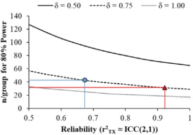
Cohen’s d = 1.0 is a “large” effect), which makes the implicit assumption of no measurement error. As such, it is important that researchers temper their predicted effect-sizes by incorpo-rating measurement error.29,30 For example, assuming alpha = 0.05 and a population difference ofδ = 0.75 between groups, most of the connectivity/thickness/volume measures in the present study would have ≥80% statistical power to detect a difference between groups when n/group ffi 30 (See Figure 1). If the primary outcome measure in a study were M1-Thalamus AD, then the observed ICC (2,1) was 0.92 par-ticipants, per group would be required to achieve 80% statis-tical power because the error in this measure effectively reduces the effect-size from an idealizedδ = 0.75 to d = 0.72. The ICC (2,1) reflects the average ratio of true variance to total variance captured by any single measurement. That is, if the ratio of the variance in “true” scores (T) to observed scores (X) is r2tx = var(T)/var(X) = 0.25 in the population,
ICC (2,1) will approximate 0.25 (large samples) regardless of the number of observations made. As such, ICC (2,1) reflects the average amount of variance in true scores that is captured by a single measurement. Presenting ICC (2,1) as a comple-ment to ICC(2,k) is important because ICC(2,k) is sensitive to the number of measurements, whereas ICC (2,1) is not and, unless experimenters are making a fixed number of repeated assessments, ICC (2,1) is most relevant to trial designs with a single pre- and posttest assessment.
Alternatively, if the primary outcome measure was PMC-Thalamus RD, then the observed ICC (2,1) was 0.68. This would mean that 43 participants are required per group, because the measurement error reduces the idealizedδ = 0.75 to d = 0.62. Thus, the n/group required to achieve statistical power varies markedly within these connectivity measures, because the reliability of a measure at a given timepoint (ICC (2,1)) varied so substantially. Naturally, as the effect-size increases (eg, from δ = 0.5 to 1.0) the n/group required to achieve 80% power decreases. However, these data show that despite generally good reliability across these neuroimaging measures, the differences in reliability still have negative con-sequences for statistical power depending on the outcome.
We also examined the amount of change in our mea-sures over 2 years. Cortical volume meamea-sures tended to show reliable decreases over time, consistent with previous research for healthy adults in this age range.31,32 For example, BA1 volume decreased by 3%, and BA4a/BA6 volume decreased by 2% on average. While these effect-sizes are relatively small, the high reliability (ie, low within-subject variance) provided adequate statistical power to detect change. Cortical thick-ness, however, did not show statistically significant changes over time, suggesting that the magnitude of change may be smaller than that of cortical volume. It is also likely that Freesurfer measurements of cortical thickness are less reliable, given that small errors in segmentation can significantly inflate thickness values for particular regions where volumetric
TABLE 6. Conti nued Scanner A (Philips) Lei v. V Scanner B (Siemens) Lo v. P Main effect of scanner Variable Overall Leiden (Lei) Vancouver (V) P -value Overall London (Lo) Paris (P) P -value F-value df P -value rh_BA6 2.62 (0.11) 2.62 (0.12) 2.62 (0.11) 0.839 2.75 (0.12) 2.77 (0.09) 2.74 (0.14) 0.358 28.7 1,89 <0.001 a Note that all variables are shown as the mean (standard dev iation) across three timepoin ts. Df = degrees of freedom. a Denotes a difference that remains statistically signi ficant following a Bonferroni correction for multiple comparisons, c = 14. Tests of site differences within a scanner (Leiden = Lei; London = Lo; Paris = P ; Vancouver = V ) weere based on Fi sher ’s LSD, collapsing across the three different timepoint s.
measures are more robust to this type of error. This could potentially impact detection of the subtle changes in thickness that may occur over a 2-year period in healthy controls.
Our data were collected on two different types of MRI scanners and despite good within-participant reliability, there was an effect of scanner type for most measures. There appeared to be a consistent trend for sites using Siemens scan-ners to produce larger values for connectivity, cortical thick-ness, and cortical volume measures than sites using Philips scanners. For volumetric and cortical thickness measures, dif-ferences between Philips and Siemens scanners are unsurpris-ing, as FreeSurfer was developed primarily on Siemens and GE scanners with the application on Philips data tested later in development.33 It is also important to note that this study was not designed to test differences between scanners or study sites, so these differences must be interpreted with caution. Different participants were measured at the different study sites, so these between-site differences are not measures of “interrater” reliability. That said, we believe that the between-scanner differences do reflect real differences between scan-ners and not merely sampling variability, given that there is demographic and anthropomorphic similarity between partic-ipants across study sites and that within-scanner differences were not statistically different (which would be more sugges-tive of differences due to sampling variability alone). Potvin et al showed that scanner type is responsible for up to 2.8% of the variance (right caudate), with most regions showing variability as low as 0.1%.34,35 This is a relatively small pro-portion of the variance, particularly when compared with age, sex, and total intracranial volume. In the current study, we have shown a clear effect of scanner type and, qualitatively, our results tend to agree with those of Duchesne et al, with higher volumes being reported for Siemens scanners com-pared with Philips scanners.36 It is difficult to compare
quantitatively our results, given that Potvin et al’s study scanned one individual, where we have larger samples, but not multiple scans per person on different scanners. Taken together, however, these results further suggest our scanner differences are real and not due to different samples at differ-ent sites.
These potential differences are especially relevant when comparing results between studies or planning multisite trials, as researchers need to account for between-site differences when pooling data sources (eg, using multilevel modeling procedures37) or when contrasting data from different sources.
Finally, we investigated differences between sites using the same scanner. Between-site differences were generally less pronounced than between-scanner differences. For example, there were no differences between the two sites using Philips scanners, although there were still some notable differences in diffusivity measures between sites using Siemens scanners. Again, we must be cautious when interpreting thesefindings, given that the design was not balanced (ie, sites were nested within scanner types and ideally we would have all partici-pants at each site scanned with each scanner, fully crossing the effects of site and scanner). In addition, these were rela-tively underpowered tests compared to those of between-scanner differences. It is clear, therefore, that despite phantom scanning, rigorous multiscanner quality control and standard-ization of training, there were still significant differences between scanners (for many measures) and between sites for a particular scanner (mostly for diffusivity measures). This rein-forces the importance of thorough training and streamlining of scanning protocols and using analyses that can account for between-site differences in large multicenter studies and clini-cal trials using MRI scanning as endpoint measures.
It is important to note that these between-site (or between-scanner) comparisons are not measures of “inter-rater” reliability, because different participants were measured at the different study sites. However, these measures are still informative because it is important to understand systematic between-participant and within-participant variability in our data.
Quantifying sources of between- and within-subject var-iability in older adults over a long timescale has important implications for clinical neuroscience. Large observational studies, for instance in Huntington’s disease or Friedreich’s ataxia, suggest that longitudinal studies with a long timescale (eg, over a number of years) are important in understanding disease-related brain alterations.4,38Differences in data collec-tion techniques, equipment, and procedures could introduce variation/noise over real biological changes that occur over time. For our healthy cohort, structural measures of thickness and volume were generally robust over time, although impacted by scanner type and, therefore, also potentially suit-able for use in a clinical trial as an exploratory endpoint.
FIGURE 1: Power analysis: The number of participants per group required to achieve 80% statistical power as a function of a hypothetical underlying effect-size (δ) and the reliability of the measurement. Reliability is expressed as the ratio of true score variance (T) to observed score variance (X), r2
TX= var Tð Þ=var Xð Þ,
TABLE 7. Effects of Scanner and Site on Cortical Volumes Scanner A (Philips) Lei v. V Scanner B (Siemens) Lo v. P Main effect of scanner Variable Overall Leiden (Lei) Vancouver (V) P -value Overall London (Lo) Paris (P) P -value F-value df P -value Left Hemisphere lh_BA1 1.8E+3 (2.2E+2) 1.7E+3 (2.0E+2) 1.8E+3 (2.4E+2) 0.321 2.0E+3 (3.0E+2) 2.0E+3 (3.0E+2) 2.0E+3 (3.0E+2) 0.094 23.16 1,87 <0.001 a lh_BA2 5.8E+3 (8.4E+2) 5.7E+3 (7.8E+2) 5.9E+3 (9.0E+2) 0.503 6.3E+3 (1.1E+3) 6.0E+3 (1.0E+3) 6.7E+3 (1.1E+3) <0.001 a 5.93 1,87 0.017 lh_BA3a 8.4E+2 (1.2E+2) 8.4E+2 (1.2E+2) 8.4E+2 (1.2E+2) 0.316 9.4E+2 (1.2E+2) 9.4E+2 (1.3E+2) 9.4E+2 (1.0E+2) 0.679 20.46 1,87 <0.001 a lh_BA3b 3.1E+3 (3.6E+2) 3.1E+3 (3.7E+2) 3.1E+3 (3.6E+2) 0.973 3.4E+3 (5.1E+2) 3.4E+3 (5.7E+2) 3.4E+3 (4.4E+2) 0.051 17.63 1,87 <0.001 a lh_BA4a 3.0E+3 (4.2E+2) 3.0E+3 (4.2E+2) 3.0E+3 (4.1E+2) 0.807 3.2E+3 (3.5E+2) 3.2E+3 (3.5E+2) 3.2E+3 (3.6E+2) 0.747 6.64 1,87 0.012 lh_BA4p 2.1E+3 (3.2E+2) 2.1E+3 (2.9E+2) 2.0E+3 (3.5E+2) 0.010 2.1E+3 (2.2E+2) 2.1E+3 (2.6E+2) 2.1E+3 (1.7E+2) 0.560 2.49 1,87 0.118 lh_BA6 1.8E+4 (2.0E+3) 1.8E+4 (2.0E+3) 1.9E+4 (2.2E+3) 0.285 2.0E+4 (2.5E+3) 2.0E+4 (2.4E+3) 2.0E+4 (2.6E+3) 0.399 22.68 1,87 <0.001 a Right Hemisphere rh_BA1 1.6E+3 (2.5E+2) 1.5E+3 (2.7E+2) 1.6E+3 (2.2E+2) 0.776 1.7E+3 (3.1E+2) 1.7E+3 (3.4E+02) 1.7E+3 (2.8E+2) 0.778 5.37 1,86 0.023 rh_BA2 4.7E+3 (8.3E+2) 4.5E+3 (8.8E+2) 4.9E+3 (7.4E+2) 0.195 4.7E+3 (9.2E+2) 4.6E+3 (9.1E+2) 4.8E+3 (9.3E+2) 0.242 0.01 1,87 0.953 rh_BA3a 8.8E+2 (1.2E+2) 8.6E+2 (1.1E+2) 9.0E+2 (1.2E+2) 0.51 1.0E+3 (2.2E+2) 9.8E+2 (1.9E+2) 1.0E+3 (2.5E+2) 0.303 13.55 1,87 <0.001 a rh_BA3b 2.4E+3 (3.4E+2) 2.4E+3 (3.8E+2) 2.5E+3 (3.0E+2) 0.842 2.7E+3 (4.7E+2) 2.7E+3 (4.9E+2) 2.8E+3 (4.4E+2) 0.398 14.29 1,87 <0.001 a rh_BA4a 2.8E+3 (3.4E+2) 2.8E+3 (4.0E+2) 2.8E+3 (2.8E+2) 0.998 3.0E+3 (4.3E+2) 3.0E+3 (4.2E+2) 3.0E+3 (4.6E+2) 0.304 8.33 1,87 0.005 rh_BA4p 1.9E+3 (2.5E+2) 1.9E+3 (2.7E+2) 1.9E+3 (2.2E+2) 0.803 2.0E+3 (3.2E+2) 1.9E+3 (2.3E+2) 2.0E+3 (3.9E+2) 0.661 3.38 1,87 0.069
Diffusion metrics do not have the same level of robustness, as they are seemingly more affected by scanner type and in terms of intersite variability. Therefore, when embarking on a longitudinal study, it is crucial to have some knowledge of the potential variability that may be introduced when investi-gating a brain structure or connectivity.
Acknowledgments
The authors thank the Track-On HD study participants and the CHDI/ High Q Foundation, a not-for-profit organization dedicated tofinding treatments for HD.
Track-On HD Investigators
A. Coleman, J. Decolongon, M. Fan, T. Koren (University of British Columbia, Vancouver); C. Jauffret, D. Justo, S. Lehericy, K. Nigaud, R. Valabrègue (ICM and APHP, Pitié- Salpêtrière University Hospital, Paris); S. Klöppel, E. Scheller, L. Minkova (University of Freiberg, Freiberg), A. Schoonderbeek, E. P ’t Hart (Leiden University Medical Centre, Leiden); C. Berna, M. Desikan, R. Ghosh, D. Hensman Moss, E. Johnson, P. McColgan, G. Owen, M. Papoutsi, A. Razi, J. Read, (University College London, London); D. Craufurd (Manchester University, Manchester); R. Reilmann, N. Weber (George Huntington Institute, Munster); H. Johnson, J.D. Long, J. Mills (University of Iowa, Iowa); J. Stout, I. Labuschagne (Monash University, Melbourne); G.B. Landwehrmeyer, I. Mayer (Ulm Univer-sity, Ulm).
Funding
This work was funded by the CHDI Foundation and the Wellcome Trust (G.R.). S.J.T. is partly supported by the UK Dementia Research Institute that receives its funding from DRI Ltd., funded by the UK Medical Research Council, Alzheimer’s Society, and Alzheimer’s Research UK. Some of this work was also undertaken at UCLH/UCL, who acknowl-edge support from the Department of Health’s NIHR Bio-medical Research Centre.
K.L. is supported by the Canadian Institutes of Health Research (PTJ 153330) and the Auburn University Internal Grants Program (170138). S.G., R.S., G.R., and S.T. receive support from a Wellcome Trust Collaborative Award (200181/Z/15/Z). All authors declare that they have no con-flicts of interest.
REFERENCES
1. Beaulieu C. The basis of anisotropic water diffusion in the nervous sys-tem— A technical review. NMR Biomed 2002;15:435-455. http://www. scopus.com/inward/record.url?eid=2-s2.0-0036868692&partnerID=40&md5=91557e2bc6e3339d2422829b 4cd1c009. TABLE 7. Conti nued Scanner A (Philips) Lei v. V Scanner B (Siemens) Lo v. P Main effect of scanner Variable Overall Leiden (Lei) Vancouver (V) P -value Overall London (Lo) Paris (P) P -value F-value df P -value rh_BA6 1.5E+4 (1.9E+3) 1.5E+4 (1.8E+3) 1.6E+4 (2.0E+3) 0.189 1.7E+4 (2.3E+3) 1.7E+4 (2.0E+3) 1.7E+4 (2.6E+3) 0.155 14.56 1,87 <0.001 a Note that all variables are shown as the mean (standard dev iation) across three timepoin ts. Df = degrees of freedom. a Denotes a difference that remains statistically signi ficant following a Bonferroni correction for multiple comparisons, c = 14. Tests of site differences within a scanner (Leiden = Lei; London = Lo; Paris = P ; Vancouver = V ) were based on Fisher ’s LSD, collapsing across the three different timepoints.
2. Orth M, Gregory S, Scahill RI, et al. Natural variation in sensory-motor white matter organization influences manifestations of Huntington’s dis-ease. Hum Brain Mapp 2016;37(12):3516-3527.
3. Poudel GR, Stout JC, Domínguez DJF, et al. White matter connectivity reflects clinical and cognitive status in Huntington’s disease. Neurobiol Dis 2014;65:180-187. http://www.scopus.com/inward/record.url? eid=2-s2.0-84894301128&partnerID=40&md5=d836fef6d2fed93 f7a0574ef9581dad3.
4. Tabrizi SJ, Scahill RI, Owen G, et al. Predictors of phenotypic progres-sion and disease onset in premanifest and early-stage Huntington’s dis-ease in the TRACK-HD study: Analysis of 36-month observational data. Lancet Neurol 2013;12(7):637-649. http://www.scopus.com/inward/ record.url?eid=2-s2.0-84877098883&partnerID=40&md5=
cad80d9ce3f7ce74d8dbce35680a81b1.
5. Tabrizi SJ, Reilmann R, Roos RA, et al. Potential endpoints for clinical trials in premanifest and early Huntington’s disease in the TRACK-HD study: Analysis of 24 month observational data. Lancet Neurol 2012;11: 42-53.
6. Paulsen JS, Nopoulos PC, Aylward E, et al. Striatal and white matter predictors of estimated diagnosis for Huntington disease. Brain Res Bull 2010;82:201-207.
7. Clerx L, van Rossum IA, Burns L, et al. Measurements of medial tempo-ral lobe atrophy for prediction of Alzheimer’s disease in subjects with mild cognitive impairment. Neurobiol Aging 2013;34:2003-2013. 8. Burton EJ, Barber R, Mukaetova-Ladinska EB, et al. Medial temporal
lobe atrophy on MRI differentiates Alzheimer’s disease from dementia with Lewy bodies and vascular cognitive impairment: A prospective study with pathological verification of diagnosis. Brain 2009;132: 195-203.
9. Harper L, Barkhof F, Scheltens P, Schott JM, Fox NC. An algorithmic approach to structural imaging in dementia. J Neurol Neurosurg Psy-chiatry 2014;85:692-698.
10. Fu Y, Talavage TM, Cheng JX. New imaging techniques in the diagno-sis of multiple sclerodiagno-sis. Expert Opin Med Diagn 2008;2:1055-1065. 11. Palacios EM, Martin AJ, Boss MA, et al. Toward precision and
repro-ducibility of diffusion tensor imaging: A multicenter diffusion phantom and traveling volunteer study. AJNR Am J Neuroradiol 2017;38: 537-545.
12. Buchanan CR, Pernet CR, Gorgolewski KJ, Storkey AJ, Bastin ME. Test-retest reliability of structural brain networks from diffusion MRI. Neuroimage 2014;86:231-243.
13. Grech-Sollars M, Hales PW, Miyazaki K, et al. Multi-centre reproducibil-ity of diffusion MRI parameters for clinical sequences in the brain. NMR Biomed 2015;28:468-485.
14. de Vet HC, Terwee CB, Knol DL, Bouter LM. When to use agreement versus reliability measures. J Clin Epidemiol 2006;59:1033-1039. 15. Guyatt G, Walter S, Norman G. Measuring change over time: Assessing
the usefulness of evaluative instruments. J Chronic Dis 1987;40:171-178. http://www.ncbi.nlm.nih.gov/pubmed/3818871.
16. Brown KE, Lohse KR, Mayer IMS, et al. The reliability of commonly used electrophysiology measures. Brain Stimul 2017;10(6):1102-1111. 17. Kloppel S, Gregory S, Scheller E, et al. Compensation in preclinical
Huntington’s disease: Evidence from the Track-on HD study. EBioMedicine 2015;2:1420-1429.
18. Glover GH, Mueller BA, Turner JA, et al. Function biomedical informat-ics research network recommendations for prospective multicenter functional MRI studies. J Magn Reson Imaging 2012;36:39-54.
19. Sled JG, Zijdenbos AP, Evans AC. A nonparametric method for auto-matic correction of intensity nonuniformity in MRI data. IEEE Trans Med Imaging 1998;17:87-97.
20. Smith SM, Jenkinson M, Woolrich MW, et al. Advances in functional and structural MR image analysis and implementation as FSL. Neuroimage 2004;23(Suppl 1):S208-S219.
21. Behrens TE, Woolrich MW, Jenkinson M, et al. Characterization and propagation of uncertainty in diffusion-weighted MR imaging. Magn Reson Med 2003;50:1077-1088.
22. Behrens TE, Berg HJ, Jbabdi S, Rushworth MF, Woolrich MW. Probabi-listic diffusion tractography with multiplefibre orientations: What can we gain? Neuroimage 2007;34:144-155.
23. Shrout PE, Fleiss JL. Intraclass correlations: Uses in assessing rater reli-ability. Psychol Bull 1979;86:420-428. http://www.ncbi.nlm.nih.gov/ pubmed/18839484.
24. Trevethan R. Intraclass correlation coefficients: Clearing the air, exten-ding some cautions, and making some request. Health Serv Outcomes Res Methodol 2017;17:127-143.
25. Kline P. The handbook of psychological testing. 2nd ed. New York: Routledge; 1999.
26. Madan CR, Kensinger EA. Test-retest reliability of brain morphology estimates. Brain Inf 2017;4:107-121.
27. Iscan Z, Jin TB, Kendrick A, et al. Test-retest reliability of freesurfer measurements within and between sites: Effects of visual approval pro-cess. Hum Brain Mapp 2015;36:3472-3485.
28. Cleary TA, Linn RL. Error of measurement and the power of a statistical test. Br J Math Stat Psychol 1969;22(1):49–55.
29. Crocker L, Algina J. Introduction to classical and modern test theory. New York: Holt, Rinehart, and Winston; 1986.
30. Sutcliffe JP. On the relationship of reliability to statistical power. Psychol Bull 1980;88(2):509-515.
31. Peters R. Ageing and the brain. Postgrad Med J 2006;82:84-88. 32. Terribilli D, Schaufelberger MS, Duran FL, et al. Age-related gray
mat-ter volume changes in the brain during non-elderly adulthood. Neuro-biol Aging 2011;32:354-368.
33. Fischl B, Dale AM. Measuring the thickness of the human cerebral cor-tex from magnetic resonance images. Proc Natl Acad Sci U S A 2000; 97:11050-11055.
34. Potvin O, Mouiha A, Dieumegarde L, Duchesne S. FreeSurfer subcorti-cal normative data. Data Brief 2016;9:732-736.
35. Potvin O, Mouiha A, Dieumegarde L, Duchesne S. Corrigendum to: “FreeSurfer subcortical normative data” [Data in Brief 9 (2016) 732–736]. Data Brief 2019;23:103704.
36. Duchesne S, Dieumegarde L, Chouinard I, et al. Structural and func-tional multi-platform MRI series of a single human volunteer over more thanfifteen years. Sci Data 2019;6(1):245.
37. Snijders AB, Bosker RJ. Multilevel analysis: An introduction to basic and advanced multilevel modeling. London: Sage; 2012.
38. Long JD, Mills JA, Leavitt BR, et al. Survival end points for Huntington disease trials prior to a motor diagnosis. JAMA Neurol 2017;74(11): 1352–1360.