HAL Id: halshs-01182200
https://halshs.archives-ouvertes.fr/halshs-01182200
Preprint submitted on 30 Jul 2015
HAL is a multi-disciplinary open access
archive for the deposit and dissemination of sci-entific research documents, whether they are pub-lished or not. The documents may come from teaching and research institutions in France or
L’archive ouverte pluridisciplinaire HAL, est destinée au dépôt et à la diffusion de documents scientifiques de niveau recherche, publiés ou non, émanant des établissements d’enseignement et de recherche français ou étrangers, des laboratoires
On Abatement Services: Market Power and Efficient
Environmental Regulation
Damien Sans, Sonia Schwartz, Hubert Stahn
To cite this version:
Damien Sans, Sonia Schwartz, Hubert Stahn. On Abatement Services: Market Power and Efficient Environmental Regulation. 2015. �halshs-01182200�
Working Papers / Documents de travail
On Abatement Services:
Market Power and Efficient Environmental Regulation
Damien Sans
Sonia Schwartz
Hubert Stahn
On Abatement Services:
Market Power and E¢ cient Environmental Regulation
Damien SANS1Aix-Marseille University (Aix-Marseille School of Economics), CNRS, & EHESS.
Sonia SCHWARTZ2
CERDI, Université d’Auvergne.
Hubert STAHN3
Aix-Marseille University (Aix-Marseille School of Economics), CNRS, & EHESS.
Abstract
In this paper, we study an eco-industry providing an environmental service to a com-petitive polluting sector. We show that even if this eco-industry is highly concentrated, a standard environmental policy based on a Pigouvian tax or a pollution permit market reaches the …rst-best outcome, challenging the Tinbergen rule. To illustrate this point, we …rst consider an upstream monopoly selling eco-services to a representative pollut-ing …rm. We progressively extend our result to heterogeneous downstream polluters and heterogeneous upstream Cournot competitors. Finally, we underline some limits of this result. It does not hold under the assumption of abatement goods or downstream market power. In this last case, we obtain Barnett’s result.
Key words: Environmental regulation, Eco-industry, Imperfect Competition, Abatement services
JEL classi…cation: Q58, D43
Email addresses: damien.sans@univ-amu.fr (Damien SANS ), sonia.schwartz@udamail.fr (Sonia SCHWARTZ ), hubert.stahn@univ-amu.fr (Hubert STAHN )
1Postal address: GREQAM, Centre de la Vieille Charité, 2, rue de la Charité, 13236 Marseille, France 2Postal address: CERDI, 65 boulevard François Mitterrand 63000 Clermont-Ferrand, France
1. Introduction
The so-called Environmental Goods and Services Sector (EGSS hereafter) and its link to environmental regulation is nowadays clearly recognized. This sector "includes the provision of environmental technologies, goods and services for every kind of use, i.e. intermediate and …nal consumption as well as gross capital formation" (Eurostats’ handbook on EGSS [13]). Even if some methodological problems remain (see the UNEP report, [35]), the EGSS is largely documented by most of the statistical institutes.4 They agree upon the fact that the size of the EGSS remains relatively moderate: the share of the EGSS gross value-added in the GDP is around 2.0% in both Europe and the US. But they also point out the notable growth rate of this sector, its capacity to generate new job opportunities and its export performance. For instance, estimates for the European Union show an increase of EGSS output per unit of GDP of 50 % between 2000 and 2011, while employment grew at around 40%.
Two other observations concerning the EGSS seem to be important. First, it is widely acknowledged that this sector is controlled by worldwide …rms like CH2M Hill, Veolia Environmental Services, Vivendi Environment or Suez Environnement. The Ecorys report [11] on the European EGSS even mentions that 10% of the companies account for almost 80% of the operating revenue. Secondly, a large share of EGSS activity is dedicated to the provision of environmental services. Environmental services represent more than 40% of this sector’s activity (see Sainclair Desgagné [33] table 2) and are largely involved in international trade.5
These two last observations motivate our paper. The question is quite simple: should we regulate a polluting industry in the same way when these …rms supply abatement goods to an imperfectly competitive eco-industry as when they supply abatement services? This raises a second question: what is the di¤erence between abatement goods and abatement services? If we follow the Eurostats’ handbook on EGSS [11]: "Services are outputs produced to order and which cannot be traded separately from their production. Services are not separate entities over which ownership rights can be established". In the context of end-of-pipe abatement, this means that the polluter buys "pollution reduction" without concerning itself about the way this task is performed: it simply outsources this activity. This is, for instance, the case for waste management, water sewerage and treatment, remediation and clean-up activities. In other words, since services are not separate entities, they cannot be used as an input in the polluter’s production process, unlike environmental goods such as …lters, scrubbers or incinerators, over which the polluter keeps some control. This simple observation fundamentally modi…es the polluter’s purchasing behavior. When
4Several empirical studies have recently sought to quantify the EGSS. For instance, the Canadian
statistical institute [34] conducts a biennial survey of the EGGS (http: //www.statcan.gc.ca /eng /sur-vey /business /1209). In Europe, Eurostats has initiated a study over 28 member states (see http: //ec.europa.eu /eurostat /statistics-explained /index.php /Environmental_goods_and_services_sector) based on a methodology described in Eutostats [13]. In 2010, the US department of commerce published a survey called "Measuring the Green Economy" [36].
he buys abatement services, i.e. pollution reduction, he only makes a trade-o¤ between the price of this service and the cost of non-compliance with an environmental act. While for environmental goods, he must also take into account the marginal rate of pollution abatement, since these goods are viewed as inputs that reduce emissions.
If the eco-industry is imperfectly competitive, the di¤erence between abatement goods and abatement services also a¤ects the expected demand for abatement and therefore the strategic behaviors of the members of this industry. For instance, under a Pigouvian tax, the purchasing behavior for abatement services is only motivated by the di¤erence between the environmental tax and the price of the abatement service. Thus, the regulator implicitly controls the market for abatement services by setting the level of the Pigouvian tax. By exploiting these particular features, we show that the regulator can obtain the …rst-best outcome simply by setting a Pigovian tax equal to the marginal damage. In other words, the …rst-best outcome can be reached with only one economic policy tool, although there are two market failures in this economy: market power on the market for abatement services and pollution. This result challenges the Tinbergen rule and suggests that the environmental agency must distinguish between the regulation of goods and the regulation of services.
To the best of our knowledge, this distinction has not been introduced into the eco-industry literature. If we invoke the previous Eurostats’ de…nition, most of the contri-butions on these vertical structures are concerned with either environmental technologies and R&D or the provision of abatement goods.
The …rst branch considers the incentives provided by environmental policy instruments for the adoption and development of advanced abatement technology (see Requate [27] for an overview). Not all of these contributions explicitly introduce an EGSS, since this requires innovation to be a private good. The studies which go in this direction often consider an innovative …rm investing in R&D to obtain a patent over a pollution-reducing new technology. Within this framework, the performance of taxes and tradeable permits are compared under various settings. Denicolo [10] and Requate [28] make these comparisons under di¤erent timing and commitment regimes. A threat of imitation is introduced by Fischer et al. [14] while Perino [25] studies green horizontal innovation, where new technologies reduce pollution of one type while causing a new type of damage. More recently, Perino [26] focuses on the second-best policies for all combinations of emission intensity and marginal abatement costs.
The second branch, which is closer to our contribution, takes as given the existence of imperfect competition in the eco-industry selling abatement goods to a polluting sector and explores the second-best regulation policy under alternative instruments. Greaker [16] and Greaker and Rosendahl [17] introduce emission standards. David and Sinclair-Desgagné [7] and Canton et al. [6] explore the case of the Pigouvian tax, the former with imperfect competition upstream and the latter with imperfect competition both upstream and downstream, while Schwartz and Stahn [32] introduce tradable pollution rights. Endres and Friehe [12] examine the impact of environmental liability laws. Some other papers like David et al. [9] or Canton et al. [5] introduce the entry or merger of …rms in the eco-industry.
Our contribution is also very close to Nimubona and Sinclair-Desgagné [24], who ini-tiate a discussion about an internal abatement e¤ort and an external procurement of abatement facilities. However, they do not depart from the Katsoulacos and Xepapadeas [20] formulation of an end-of-pipe pollution which is common to almost all papers on the eco-industry, according to which emissions depend on the levels of production and abatement. Most of these papers also assume that abatement facilities have decreasing returns. In other words, they function as an input and not as a service, which would have constant returns.6 This is why the …rst-best outcome can be obtained with only one
instrument, contrary to David and Sinclair-Desgagné [8], who introduce both Pigouvian tax and subsidy.
The intuition behind our main result is quite simple. If a Pigouvian tax is imposed, a polluter purchasing an eco-service either (i) prefers to pay the tax if the price of the abatement service is higher, (ii) decides, in the opposite case, to fully abate the pollution issued from its equilibrium production level, or (iii) is indi¤erent between the two if the price and the tax are equal. This implies that the demand for eco-services becomes perfectly elastic over a range of quantities which depends on the tax level, so that any monopoly selling these services loses - at least partially - its market power. If the regulator is able to set a tax level with the property that the monopoly solution belongs to this range of quantities, he clearly destroys upstream monopoly power and has the opportunity, if the downstream polluting market is competitive, to reach a …rst-best allocation. Owing to the structure of the demand for eco-services, this situation occurs when the monopoly has an incentive to set the highest price for which the demand is positive, i.e. the tax level, and to supply, due to marginal cost concerns, a quantity of services lower than the one corresponding to full pollution abatement, so that we end up in a situation in which the price equates the tax level and the marginal cost. If the e¢ cient abatement level does not require full abatement, it remains for the regulator to set the Pigouvian tax at the optimal marginal damage in order to obtain the …rst best.
This argument clearly holds with homogeneous competitive polluters, an eco-service monopoly and an optimal abatement level that does not require full abatement. That is why we start with this benchmark case. We then show that our argument can easily be extended in order to (i) include the "boundary" solutions corresponding to e¢ cient full pollution abatement,7 (ii) take into account regulation by a pollution permit market, and
(iii) consider polluters who are heterogeneous with regard to their production costs and emissions. The extension of our analysis to Cournot competition in the eco-industry is less obvious, which is why we have dedicated a whole section to this study. As both main assumptions nevertheless remain in this new case - upstream eco-services and downstream
6Our end-of-pipe emission reduction technology can therefore be viewed as a particular case of the
Katsoulacos and Xepapadeas [20] emission function in which the abatement good has constant returns to scale. To the best of our knowledge, this case has not been explored, probably for technical reasons: standard di¤erential calculus does not really apply and corner solutions emerge.
7The case of e¢ cient full downstream pollution abatement is particularly conceivable if the upstream
perfect competition - our result still holds. We …nally exhibit some limits of our analysis, taking into account …rst abatement goods and then downstream imperfect competition. This last section enables us …rstly, to underline the fact that the existence of eco-services is crucial, and secondly, to extend Barnett’s results [2] on Pigouvian taxation to eco-service industries.
The structure of the article is as follows. Section 2 describes the model. Section 3 presents the simplest case: downstream homogeneous polluters and an upstream monopoly. Section 4 introduces some straightforward extensions: downstream full abatement, pol-lution permit market and heterogeneous downstream …rms. Section 5 is dedicated to Cournot competition in the eco-industry. Section 6 challenges both main assumptions: environmental services and downstream perfect competition. Finally, some concluding remarks are given in Section 7 and technical proofs are relegated to an appendix.
2. A basic model of environmental services
We …rst present the main assumptions of the model and then we characterize the …rst-best allocation.
2.1. The main assumptions
We consider a standard polluting industry …rst characterized by a representative …rm which produces a quantity Q at a given cost c(Q) and latter by heterogeneous …rms. This cost is increasing and convex (i.e., c0(Q) > 0 and c00(Q) > 0), inaction is allowed (i.e., c(0) = 0), c0(0) = 0 and lim
q!+1c0(q) = +1. This activity is polluting. Emissions
are given by "(Q), an increasing and convex function (i.e., "0(Q) > 0 and "00(Q) > 0)
which satis…es "(0) = 0, "0(0) = 0 and limq!+1"0(q) = +1. This dirty …rm can buy
environmental services to reduce its "end-of-pipe" pollution. In doing so, a part A of its emissions is abated by a specialized external …rm and the remaining pollution is E = maxf"(Q) A; 0g.
The eco-services are supplied on a non-competitive market at price pA. We initially
assume that these services are provided by a monopoly. This …rm is characterized by an increasing and convex cost function and inaction is allowed (i.e., 0(a) > 0, 00(a) > 0 and (0) = 0). We also assume that 0(0) = 0 to ensure that the eco-service market is
activated when an environmental policy is implemented.8
The environmental damage induced by the remaining emissions E is measured by a standard damage function D(E). As usual, this function is increasing and convex (i.e., D0(E) > 0and D00(E) > 0) and without emission there is no damage (i.e., D(0) = 0). We
8A discussion about the emergence of an eco-industry related to the fact that 0(0) > 0 can be found
also set D0(0) = 0. This last assumption is essentially made for convenience: it ensures
that full abatement never occurs at an e¢ cient allocation.9
Finally, to close the model, we introduce an inverse demand function for the polluting goods P (Q). This function is decreasing (i.e., P0(Q) < 0) and veri…es that limQ!0P (Q) =
+1 and limQ!+1P (Q) = 0. 2.2. The …rst-best allocation
Under these assumptions, a …rst-best allocation is given by:
Qopt; Aopt 2 arg max
Q;A 0
Z Q 0
P (q) dq c (Q) D (maxf" (Q) A; 0g) (A) (1)
This is typically a non-smooth optimization problem, but remember that we have as-sumed that D(0) = 0 and D0(0) = 0. The …rst equality ensures that the optimal
level of abatement cannot be larger than emissions because abatement is costly, hence " (Qopt) Aopt 0, while the second combined with the positivity of the marginal cost of
abatement ensures that this inequality holds strictly. Consequently, the …rst-best alloca-tion is characterized by the usual …rst order condialloca-tions:
P (Qopt) c0 Qopt D0 " Qopt Aopt :"0 Qopt = 0 (2) D0 " Qopt Aopt 0(Aopt) = 0 (3)
Let us now introduce the function (Q) = P (Q) c"0(Q)0(Q) de…ned on [0; Qmax] where Qmax
stands for the optimal level of production without environmental damage (i.e., P (Qmax) =
c0(Q
max)). This function measures, for each Q Qmax, the marginal bene…t from an
additional unit of pollution. Therefore an optimal allocation has the property that the marginal bene…t of pollution is equal to (i) the marginal damage and (ii) the marginal cost of abating an additional unit of pollution:
(Qopt) = D0 " Qopt Aopt = 0(Aopt) (4) For later use, let us also notice this marginal bene…t is decreasing and (Qmax) = 0 so
that 1 : [0; +
1] ! [0; Qmax] is de…ned.
3. Upstream monopoly power and …rst-best regulation
Let us …rst show that a policy maker reaches the e¢ cient allocation with a standard Pigouvian tax scheme even if the provider of environmental services has a monopoly power. To illustrate this point, we proceed in three steps. We …rst introduce a Pigouvian tax and
9If the marginal damage at zero is high enough and/or the marginal abatement cost is not too excessive,
the "end-of-pipe" pollution assumption, i.e., E = max f"(Q) A; 0g, can lead to an e¢ cient allocation requiring full abatement (see Sans et al. [30] for a discussion). In Section 4.1, we extend our result to this case, but this requires additional discussions which are not central to our main argument.
compute the inverse demand for abatement services under a downstream market clearing assumption. This brings us, in a second step, to the characterization of the behavior of the upstream monopolist whatever the Pigouvian tax is. It remains, in the last step, to show that a Pigouvian tax equal to the marginal damage regulates both environmental and market power ine¢ ciencies.
3.1. The (inverse) demand for abatement services
The competitive dirty …rm chooses its production supply and its demand for the abatement good by solving:
max Q 0 8 > > > < > > > : pQ Q c (Q) min A 0fpA A + maxf" (Q) A; 0gg | {z } =CA(pA; ;Q) 9 > > > = > > > ; (5)
An inspection of the cost minimization part of this program shows that the conditional demand for abatement services never exceeds " (Q) and that the objective function is linear in A on [0; " (Q)]. Both properties imply that the conditional demand for abatement services is either 0 or "(Q) when pA> or pA< respectively, and any quantity within
[0; " (Q)] if pA = . Hence, the abatement cost is given by CA(pA; ; Q) = minfpA; g
"(Q). The optimal product supply therefore solves the following FOC:
pQ c0(Q) minfpA; g "0(Q) 0 (with equality if Q > 0) (6)
If we now introduce the market clearing condition for the …nal good, we can replace pQ by
P (Q), and, using the above de…nition of (Q) ;i.e., the marginal bene…t of an additional unit of pollution, this quantity is given by:
P (Q) c0(Q)
"0(Q) = minfpA; g ) Q (pA; ) =
1(min
fpA; g) (7)
and the demand for abatement services becomes:
Ad(pA; ) = 8 < : 0 if pA> [0; " ( 1( ))] if p A= " ( 1(p A)) if pA< (8)
The last two equations (Eqs (7) and (8)) stress the consequence of introducing abatement services as opposed to abatement goods. In the …rst case, the dirty …rm simply delegates its abatement activity to another …rm, while in the second case, the …rm buys additional inputs which enter the production process and help to reduce pollution in a more or less e¢ cient way. This means that the dirty …rm considers that the marginal pollution abatement of an environmental service is constant (even equal to one). Its purchasing is therefore simply motivated by the di¤erence between the price of the service and the Pigouvian tax. If the price is higher than the Pigouvian tax, it is optimal to pay the
tax and to adjust the output level due to this additional cost. In the opposite case, the …rm totally abates its emissions but adjusts the production level, as previously, since the abatement price now enters the global marginal production cost.
By introducing abatement services instead of abatement goods, we therefore obtain a particular abatement demand curve (see Eq (8)) characterized by a ‡at part when the price is equal to the Pigouvian tax and a decreasing part for prices lower than this tax and corresponding to full abatement. When this price goes to 0, we even observe, by our above de…nition of , that the equilibrium production level will be equal to Qmax, the
production level without regulation. In other words, this demand has an upper bound given by Ad(0; ) = " (Q
max) which is independent of , so that the associated inverse
demand function is:
PA(A; ) = max min ; " 1(A) ; 0 (9)
3.2. The monopoly provision of environmental services
We now address the question of how a monopoly behaves in the face of such an inverse demand curve. Since the demand is bounded from above by " (Qmax) which is reached at
a zero price, its production choice can be restricted to A 2 [0; " (Qmax)] and its optimal
decision solves:
max
A2[0;"(Qmax)]fmin f ; p(A)g
A (A)g (10)
where p (A) = (" 1(A)) is the inverse demand curve corresponding to full pollution
abatement that occurs if the Pigouvian tax is larger than this price.
Since we maximize a continuous function on a compact set, existence is not a real issue. But the characterization of this solution requires some additional concavity properties. So let us assume, as usual for a monopoly, that ep(A) = p
0A
p , the elasticity of p(A) is
decreasing and limA!"(Qmax)ep(A) is larger than 1.
10
The inverse demand curve min f ; p(A)g nevertheless exhibits a ‡at part since the dirty …rm only reacts to prices lower than the Pigouvian tax. We are therefore dealing with a non-smooth optimization problem leading to several regimes delineated by thresholds which are related to the levels of the Pigouvian tax.
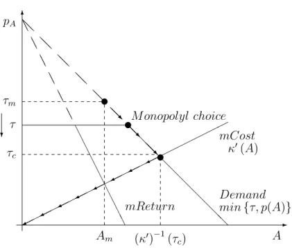
To get some intuitions (see Figure 1), let us …rst introduce the production level Am.
This corresponds to the monopoly solution under full pollution abatement behavior by the dirty …rm, i.e., the quantity that equates the marginal cost to the marginal revenue computed with p(A). The price associated with this full abatement case is therefore given by p(Am) = 1+ep1(Am) 0(Am), where 1+ep1(Am) stands for the standard margin taken by a
10Of course, the reader may object that these assumptions are not set on the primary data, especially
given that p(A) = " 1(A) . Other su¢ cient conditions can be introduced, such as 2e
"+ e 0 e"0 > 0
-6 @@ @@ @@ @@ @@ @ @ @ @ @ @ @ @ @ @ AA AA AA AA AA AA A A A A A A A A A A pA m ? c Am ( 0) 1( c) A M onopolyl choice mCost 0(A) Demand minf ; p(A)g mReturn u u u @@R @@R @@R @@R @@R @@R
Figure 1: The monopoly solution as decreases
monopolist. But this situation only occurs if the Pigouvian tax is higher than this price, i.e., p(Am), otherwise the dirty …rm pays the tax instead of abating pollution. This
means that there exists a tax rate tm implicitly given by:
m = 1+ep(p11( m))
0(p 1(
m)) (11)
for which p(Am) = m, and we can conclude that, for > m, the monopoly always
provides Am units of abatement services.
If the tax rate is lower than m, the monopoly is unable to reach this optimal outcome
simply because the monopoly price associated with full abatement is not reachable. In this case, this …rm has an incentive to choose the solution that leads to the highest price p = at the production level A = p 1( ), i.e., to remain at the kink in the demand
function. But this behavior is only optimal for prices p = which are larger than the marginal production cost, i.e., 0(p 1( )). If this is not the case, the …rm will adjusts
its behavior to equate the tax rate with the marginal cost. This means that there exists another threshold c< m with the property that 8 < c, the monopoly adopts, in some
sense, a competitive behavior. This new threshold is given by:
c= 0(p 1( c)) (12)
From this discussion, we conclude that:
Lemma 1. Under our assumptions, (i) the monopoly problem (Eq 10) has a unique so-lution for each tax rate, (ii) there exist two unique thresholds c and m which solve Eq
(12) and Eq (11) respectively, (iii) the monopoly provision of abatement services is, for any tax , a continuous function given by:
Am( ) = 8 < : ( 0) 1( ) if < c p 1( ) = " ( 1( )) if 2 [ c; m] Am = p 1( m) = " ( 1( m)) if > m (13)
(iv) the price of these services is PAm( ) = minf ; mg, and (v) from Eq (7), the production
of the dirty good is:
Qm( ) = 1(minf ; mg) (14)
3.3. The e¢ cient regulation of emissions
The previous lemma has an interesting consequence: for any tax rate lower than c,
the monopoly behaves like a competitive …rm. This …rm equates its marginal cost with the tax rate, which is nothing other than the price of the abatement services. Since the polluting …rm also behaves competitively, the regulator should be able to implement the …rst-best allocation, by selecting, as in a competitive case, a Pigouvian tax equal to the marginal damage of pollution, i.e., by setting opt = D0(" (Qopt) Aopt).
This point is obvious as long as opt <
c. In this case, we know, from Eq (13), that
the monopoly provision of environmental services veri…es 0(Am( opt)) = opt, while Eq
(14) says that (Qm( opt)) = opt, and since and 0 are both monotonic, we conclude,
by identi…cation with Eq (4), that Qm( opt) = Qopt and Am( opt) = Aopt, i.e., that the
…rst-best allocation is reached.
It therefore remains to verify that opt <
c. Intuitively, c is by de…nition (see Figure
1) (i) the highest tax level at which the monopoly behaves competitively and (ii) the lowest rate at which full abatement occurs, so that any tax < c induces perfect competition
and partial abatement. Since there is also partial abatement at the optimum, opt should
be one of them. If this is not the case, i.e. opt
c , we know from the de…nition of the
threshold c (see Eq (12)) that: opt 0(p 1 opt )
, ( 0) 1 opt " 1 opt since p(A) = " 1(A) (15)
Moreover, by Eq (4), which characterizes the …rst-best solution, ( 0) 1( opt) = Aopt and
1( opt) = Qopt, so that Aopt " (Qopt). But from our discussion about the e¢ cient
allocation, we know that the assumptions D(0) = D0(0) = 0 ensure that there is always
a residual pollution at the optimum, i.e., that " (Qopt) > Aopt. We can therefore say:
Proposition 1. Even if an upstream monopoly controls the price of the environmen-tal services while the downstream commodity market remains competitive, the regulator reaches the …rst-best by setting the Pigouvian tax at the marginal damage of the emissions (evaluated at the …rst-best), i.e., by setting opt = D0(" (Qopt) Aopt).
4. Some straightforward extensions
The previous result suggests that the existence of a residual pollution at the optimal outcome is a crucial assumption. However, as we will see, this is only a simplifying assumption: an identical result can be obtained for D0(0)6= 0. In this section, we can also
examine whether the result is maintained when the regulator uses a di¤erent incentive-based mechanism such as tradable pollution permits. The answer is again yes as long as this new market is competitive. Finally, we relax the representative polluting …rm assumption and investigate heterogeneous polluters.
4.1. E¢ cient regulation and full abatement
To illustrate this point, let us return to the construction of the e¢ cient outcome and relax D0(0) = 0 11. This outcome solves the optimization program (Eq (1)) introduced in Section 2.2. But if we only assume that D(0) = 0; we can only argue that " (Q) A 0, (i.e., without a strict inequality). The interior …rst-order optimality conditions given by Eqs (2) and (3) must therefore be amended. If denotes the associated Lagrangian multiplier, the new FOC become:
8 < :
P (Qopt) c0(Qopt) (D0(" (Qopt) Aopt) ) "0(Qopt) = 0
D0(" (Qopt) Aopt) 0(Aopt) = 0 (" (Qopt) Aopt) = 0 and 0
(16)
If the constraint is not binding, we are, of course, back in the case of partial abatement, analyzed above. So let us concentrate on the case in which > 0. In this situation, the …rst and second conditions of system (16) suggest that an e¢ cient allocation has the property that the marginal bene…t (Qopt)of an additional unit of pollution must be equal
to the marginal abatement cost. But to achieve full abatement, this marginal bene…t only needs to be smaller than the marginal damage of the …rst unit of pollution. This situation essentially occurs if D0(0) is high enough. In this case, the e¢ cient allocation veri…es:
Eopt = " (Qopt) Aopt = 0
(Qopt) = 0(Aopt) < D0(0) (17)
instead of the interior condition introduced in Eq. (4).
Let us now return to the monopoly case. Since the marginal damage never enters the de…nition of the di¤erent behaviors, the monopoly outcome depicted in Lemma 1 remains unchanged. This means that we simply have to ensure that the regulator is able to obtain the …rst-best solution when it is optimal to abate all the pollution (i.e. for > 0).
So let us assume that he sets the Pigouvian tax at opt = c given by Eq (12). From
Lemma 1, the equilibrium abatement and production levels are Am( c) = " ( 1( c))
and Qm( c) = 1( c), so that the …rst optimality condition of Eq (17) is satis…ed. It
11This situation is, for instance, met when the damage function is linear. Full abatement is required
then remains for us to use the de…nition of c to verify the second condition. This is c= 0(p 1( c)), so that (Qm( c)) = 0(Am( c)). We can therefore note:
Proposition 2. Assume that the marginal damage of the …rst unit of pollution is su¢ -ciently large for full abatement to become the e¢ cient outcome. If the regulator sets the Pigouvian tax at opt = c given by Eq (12), he again obtains the …rst-best outcome. 4.2. Pollution permit market
Let us now verify that our result also holds if the regulator implements a pollution permit market instead of a Pigouvian tax. To illustrate this point, let us return to the monopoly case depicted in Section 3 and introduce a competitive market of pollution rights. The regulator sets the pollution cap E. Without loss of generality, we assume that pollution permits are sold by means of an auction.12 One right corresponds to one
unit of emission and the competitive price of these rights is denoted by pE.
At the agent level, the competitive permit price operates like a Pigouvian tax. Under our assumptions, the results obtained in Section 3 concerning the inverse demand and the supply of abatement services by the monopoly extend to this case: it simply remains for us to replace the Pigouvian tax by the price pE of the emission rights. Thus, our result
is maintained if there exists a pollution cap Eopt with the property that the equilibrium price of the pollution rights is equal to the optimal level of the Pigouvian tax introduced in Proposition 1. This nevertheless leaves two questions open: (i) what is the value of this pollution cap?, and (ii), more crucially, is pE = opt the unique equilibrium of the
pollution permit market when this cap is set? Otherwise there may be several equilibria, some of them being ine¢ cient.
To answer these two questions, let us observe that in our new setting, the quantities introduced in Eqs (13) and (14) of Lemma 1 describe the equilibrium allocation conditional on each pollution permit price pE. So if we want to look at the global equilibrium of this
vertical structure with tradable rights, we must clear the permit market. The demand for pollution rights is given by:
ED(pE) = " (Qm(pE)) Am(pE) (18)
and we observe that for any price pE c there is full abatement, hence:
ED(pE) =
" ( 1(p
E)) ( 0) 1(pE) if pE < c
0 if pE c
(19)
Now let us recall from our earlier discussion that opt = D0(" (Qopt) Aopt) <
c. Hence,
the optimal pollution cap must be:
Eopt = " 1 opt ( 0) 1 opt (20)
12For simplicity, we do not introduce the initial distribution of pollution permits explicitly. Following
Montgomery [22], the competitive equilibrium of a pollution permit market is obtained irrespective of the initial distribution of permits.
Moreover, to ensure that pE = opt is the unique equilibrium, let us observe that the
demand for tradable rights is decreasing for all pE < c:
dED(p E) dpE = " 0( 1(p E)) 0( 1(p E)) 00 ( 0) 1 (pE) 1 < 0 (21)
since under our assumptions, "; "0 > 0 and 0 < 0. We can therefore say:
Proposition 3. If pollution is regulated by a market of pollution rights, the regulator also achieves an e¢ cient allocation by choosing the optimal pollution cap Eopt given by
Eq. (20).
4.3. Heterogeneous polluters
Finally, it is also interesting to verify whether this result extends to heterogeneous polluters. So let us introduce m polluting …rms, indexed by j, with di¤erent cost and emission functions, cj(q) and "j(q), each of them satisfying the assumptions introduced
in Section 2. All the other assumptions are maintained, especially those concerning the marginal damage at 0, so that an e¢ cient allocation is now given by:
8j P (Pmj=1q opt j ) c0j q opt j D0 Pm j=1"j q opt j A opt :"0 j q opt j = 0 (22a) D0 Pmj=1"j qoptj A opt 0(Aopt) = 0 (22b)
The intuition behind this extension is quite simple. Even if the polluting …rms are heterogeneous in costs and/or emissions, they invariably choose their level of abatement by comparing the price pA with the Pigouvian tax . One can therefore expect the
aggregate demand for abatement goods to behave in the same way: no abatement if pA > , full abatement denoted Af(pA) if pA < and any situation between the two if
pA= . Moreover, if the demand on the domain corresponding to full abatement is again
decreasing and bounded from above, the inverse demand has the same structure as that obtained in Section 3.1. So, with similar assumptions on its elasticity, the properties of the monopoly outcome provided in Lemma 1 should extend to the case of heterogeneous polluters.
The main weakness of this argument is that the computation of the aggregate level of abatement corresponding to full pollution reduction (Af(pA)) and, more generally, the
construction of the market-clearing production levels for all and pA, are now trickier.
In fact - as in Section 3.1 - it is easy to compute the individual conditional demand for abatement services and the cost function related to this activity. But to compute the market-clearing production level, we now face a system of m equations, since for each …rm, the price of the polluting good is equal to the full marginal cost including abatement cost. In other words, these individual production levels solve:
8j = 1; : : : ; m P Pmj=1qj = c0j(qj) + minfpA; g "0j(qj) (23)
Lemma 2. Under our assumptions on demand, costs and emissions, the system of Eqs. (23) admits a unique solution (qj(k))mj=1 for each constant k = min fpA; g 0.
More-over, Af(pA) =
Pm
j=1"j(qj(pA)) - the total quantity of abatement good which induces
full pollution reduction - is decreasing (for all pA ) and bounded from above by
Amax =Pmj=1"j(qj(0)).
It …nally remains to verify that the Pigouvian tax opt = D0 Pm j=1"j q
opt
j Aopt
(i) is lower than the highest tax h
c that induces competitive behavior by the abatement
producer and (ii) can achieve the …rst-best outcome.13 The …rst part is obvious. If opt < h
c, the eco-service …rm equates its marginal cost with the Pigouvian tax, i.e., opt= k0(A)so that the second e¢ ciency condition (Eq. (22b)) is satis…ed. Since, in this
case, the price of the abatement good is opt, the set of Eqs 23 describing the equilibrium
production levels corresponds exactly to the …rst e¢ ciency condition (Eqs. (22a)). If opt h
c, this implies, by the de…nition of ch, that the tax opt is higher than the
marginal abatement cost which induces full abatement at price pA = opt, i.e., opt >
k0(Af( opt)). This again implies that one reduces, at the optimum, more pollution than
the existing level, which is impossible. We can therefore state that:
Proposition 4. Even if the polluting sector is composed of heterogeneous …rms, espe-cially in terms of their emissions, the regulator can neutralize the monopoly power on the abatement service market and obtain the …rst-best solution by setting the tax rate at the marginal damage.
5. Cournot competition in the eco-industry
Let us now restore the representative polluting …rm assumption, but now introduce Cournot competition in the eco-service industry. There are now n heterogeneous …rm indexed by i in the eco-industry, each characterized by a cost function i(a). Seeing that
all the other assumptions are maintained, an e¢ cient allocation now veri…es:
8i = 1 : : : ; n (Qopt) = D0 " Qopt Pni=1aopti = i a opt
i (24)
Could we again implement the …rst-best allocation by setting the Pigouvian tax at
opt = D0(" (Qopt) Pn
i=1aopt)? To answer this question, we …rst study the best
re-ply of these Cournot players, since the behavior of the polluting …rm remains unchanged by construction.
13This threshold h
c is now de…ned ch= 0 Af( ch) and using a similar argument to that used in the
5.1. The best reply of a …rm
The main di¢ culty appears at that stage. The di¤erent thresholds which characterize the behavior of a monopoly now come out during the computation of the best response and are linked to the behavior of the opponents. So instead of dealing with a piecewise continuous monopoly solution, we have, even if the intuition is maintained, to manage piecewise continuous best responses.
If we denote by A i =
Pn j=1;j6=ia
opt
j the aggregated abatement supply of the opponents,
this best response is given by:
BRi(A i; )2 arg max
ai fmin f ; p(a
i+ A i)g ai i(ai)g (25)
where p(A) = (" 1(A))stands for the inverse demand corresponding to full abatement behavior of the polluting industry. To gain some intuition about BRi(A i; ), we
intro-duce br(A i), the best response obtained when the demand always corresponds to full
abatement behavior, i.e., with p(a). This is de…ned by: br(A i) = max
ai2[0;"(Qmax)]
p(ai+ A i) ai i(ai) (26)
and solves:
p0(ai+ A i) ai+ p(ai+ A i) 0(ai) = 0 (27)
We know that (i) bri("(Qmax)) = 0, since p ("(Qmax)) = 0, (ii) bri(0) = Am < "(Qmax)the
monopoly solution and (iii) bri is decreasing as long as e(p0) > 1, the elasticity of p0 is
larger than 1.
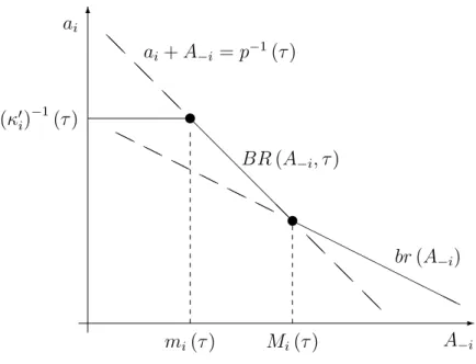
We now try to understand, at least graphically - see Figure 2 - what happens when the constraint on the price, i.e. p(ai+ A i) , begins to matter.
In Figure 2, we consider the unconstrained best response bri(A i) and the 45 line
given by ai + A i = p 1( ). Since p(a) is decreasing, this linear constraint provides, for
each A i, the minimum production level of …rm i ensuring that the price is lower than ,
or in other words, the minimal production level that preserves market power. So, as long as the best reply bri(A i)lies above this line, the …rm is able to exert market power, i.e.,
his best reply is BRi(A i; ) = bri(A i). This remains true until bri(A i) cuts this line.
This intersection occurs when the A i is equal to Mi( ) which is de…ned by:
p0(p 1( )) p 1( ) Mi( ) + 0i p
1( ) M
i( ) = 0 (28)
If A i Mi( ), …rm i is, as in the monopoly case, unable to manipulate the price. This
is why it becomes optimal to produce the quantity that keeps the price at . In other words, the best reply is BRi(A i; ) = p 1( ) A i. However, as A i decreases, …rm i
increases its market share while the price remains constant at . It is therefore possible for the marginal production cost to be higher than the price. This situation occurs for all A i < mi( ) with mi( ) solution to:
0 i p 1( ) m i( ) = , mi( ) = p 1( ) ( 0i) 1 ( ) (29)
-6 @@ @@ @@ @ @ @ @ @ @@ @@ @@ @@ HH HH HH HH HHH H H H H H H H H H H H H u u ai+ A i = p 1( ) BR (A i; ) br (A i) mi( ) Mi( ) A i ai ( 0 i) 1 ( )
Figure 2: The best response of Firm i
In this last case, the best reply depicts a competitive behavior and is given by BRi(A i; ) =
( 0 i)
1
( ). Moreover, by construction, it is immediate that mi( ) Mi( ).
This explanation nevertheless requires that (i) the line ai + A i = p 1( ) crosses
bri(A i) at a unique positive point and (ii) p 1( ) ( 0i) 1
( ) 0, otherwise some of these cases are vacuous. A formal construction of the best response is provided in the appendix. We show that the case depicted in Figure 1 only occurs when the rate is lower than ci given by ci = 0i(p 1( ci)), i.e., the upper bound of the tax rates at which
…rm i adopts a competitive behavior. But it is essentially this set of taxes in which we are interested. This is why we only spell out the characterization of the best reply for
i c.
Lemma 3. For any tax rate < ci and any A i 2 [0; " 1(Qmax)], the best response of an
eco-service …rm is given by:
BR(A i; ) = 8 < : ( 0i) 1( ) if A i < mi( ) p 1( ) A i if mi( ) A i Mi( ) bri(A i) if A i Mi( ) (30)
Moreover, this best response is continuous and, since e(p0) > 1, it is also non-increasing
with A i.
5.2. Cournot equilibrium and e¢ cient taxation
From the previous Lemma, we essentially learn that competitive behavior is part of the best response of …rm i when ci. So we will now concentrate on taxes smaller than
min
Lemma 4. For any tax < min
c , the unique equilibrium supply of eco-services is, for
each …rm, aC
i ( ) = ( 0i) 1
( ), while the price of these services is PC
A ( ) = . From Eq
(7), we observe that the production of the dirty good is QC( ) = 1( ).
The existence part of this result is obvious. Since < min
c , then 8i, < 0i(p 1( ))
by the de…nition of ci or equivalently 8i, ( 0i) 1
( ) < p 1( ). We can therefore say that:
8i Aci = n X j=1;j6=i 0 j 1 ( ) < p 1( ) ( 0i) 1( ) = mi( ) (31)
This means from Eq. (30) that playing aC
i = ( 0i) 1
( ) is a best response for each …rm. Concerning uniqueness, let us …rst observe that the best response is bounded from above by ( 0
i) 1
( ). So if there exists another equilibrium, say bC, there must be at least one …rm
i0 such that bCi0 <
0 i0
1
( ) and, due to the upper bound, Bc i0 Pn j=1;j6=i0 0 j 1 ( ). But this leads to a contradiction, since for < min
c , we have as before that Bci0 < mi0( ),
so that bCi0 =
0 i0
1
( ) should be the best response.
Let us now assume that the regulator sets opt = D0 " (Qopt) Pn i=1a
opt
i . If opt min
c , the Cournot equilibrium meets the …rst-best conditions given by Eq. (24) since, by
Lemma 4, we have:
8i = 1 : : : ; n QC( opt) = opt = 0i aCi ( opt) (32) It remains for us to verify that opt min
c . If this is not the case, there must exist at least
one agent, say i0, for which opt > 0i0(p
1( opt)). But this implies, for our characterization
of an optimal allocation (Eq. (24)), that: aopti
0 =
0 i0
1
( opt) > p 1 opt = " 1 opt = "(Qopt) (33) so thatPni=1aopti
0 > "(Q
opt), since all the aopt
i 0. In other words there is, at the optimum,
more abatement than emissions, which is a contradiction. We can therefore say:
Proposition 5. If there is Cournot competition in an eco-service industry and pure com-petition in the polluting sector, the …rst-best allocation can be reached by setting the tax rate to the marginal damage as usual.
6. Two main limits of the result
We have extended our leading case of Section 3 to various settings. Both main as-sumptions nevertheless remained: an upstream non competitive market of eco-services and a downstream competition polluting industry. In this section, we show that both assumptions are crucial. We …rst introduce a counter example showing that our result cannot be extended to abatement goods. In a second step we introduce downstream monopoly power. Due to this new market imperfection, the …rst-best allocation cannot be implemented. In this case, we show that the optimal Pigouvian tax must be lower than the marginal damage, thus …nding Barnett’s result [2].
6.1. Abatement goods versus abatement services
Our results only apply for environmental services, whereas most of the literature con-siders environmental goods. In this latter case and under an "end-of-pipe" pollution as-sumption (see Katsoulacos and Xepapadeas [20]), the emissions "(Q; A) are for the dirty …rm negatively correlated with the use of abatement goods. The marginal productivity of abatement goods ( @A"(Q; A)) therefore matters in the abatement choice, contrary to
abatement services for which the purchase decision is only based on the di¤erence between the environmental tax and the price. As we will show, this strongly reduces the control that the regulator has over the equilibrium and limits implementation of the …rst-best allocation.
As the case of abatement goods is largely documented in the literature under alter-native sets of assumptions, we simply illustrate our purpose by a (counter) example to highlight what changes compared with eco-services.
Example 1. We consider (i) quadratic cost functions, i.e., c(Q) = 1 2Q
2 and (A) = 1 2A
2,
(ii) a linear demand P = 1 Q, (iii) a linear damage function D(E) = 0:2E and (iv) an emission function "(Q; A) = maxnQ pA; 0o which is now "non-linear" in abatement. If we construct the inverse demand for abatement goods as in Section 3.1, we observe, after some computation, that the conditional demand for abatement goods and the cost associated with this activity are given by:
A(pA; ; Q) = min Q2; 2p A 2 CA(pA; ; Q) = ( pAQ2 if Q 2p A Q 2p2 A if Q > 2pA (34)
As expected, the conditional demand does not move from full abatement (here Q2) to
no abatement, since 2p
A
2
is a demand for partial pollution reduction. Moreover, the marginal cost @QCA associated with this activity is no longer linear in quantities, since
@QCA = minf2pAQ; g. This drastically modi…es the computation of the dirty good
market clearing condition, which is given by:
P (Q) = dc dQ + @CA @Q , 1 Q = Q + minf2pAQ; g , Q(pA; ) = 1 2(1+pA) if pA (1 + pA) 1 2 else (35)
It follows that the demand for abatement goods consistent with market clearing and the inverse demand curve are:
A(pa; ) = min 2(1+p1 A) 2 ; 2p A 2 PA(A; ) = ( 2pA if A < 1 2 2 1 2pA 1if A 1 2 2 (36)
Since 2p1
A 1 stands for p(A), the inverse demand under full abatement, this inverse
demand can be written as PA(A; ) = min
n p(A);
2pA
o
. Clearly, this expression di¤ers from min fp(A); g. The monopoly is now able to exert market power on the whole range of its inverse demand. The ‡at part disappears but a kink remains. This is why the monopoly solution nevertheless leads to three di¤erent outcomes: (i) the monopoly solution under partial abatement for small taxes, (ii) a solution which sticks in the kink of the inverse demand curve, and (iii) the monopoly strategy under full abatement for high taxes. It can be shown, in this example, that:
Am( ) 8 > < > : 4 2=3 for < 0:2291 1 2 2 for 2 [0:2291; 0:5265] 0:0561 for > 0:5265 and Qm( ) 1 2 for 0:5265 0:2368for > 0:5265 (37) Moreover, a simple computation shows that Aopt = 0:2 and Qopt = 0:4. As Am( ) is
bounded from above by 0:1485, the …rst-best outcome is unreachable simply because the monopoly can now take a margin in the case of full and partial pollution abatement. 6.2. Downstream market power and Barnett’s result
As we will see, our result is also limited by the number of market failures and/or imper-fections that the regulator controls. We have shown that one instrument, the Pigouvian tax, can regulate the environmental externality in the dirty sector and the imperfect com-petition problem in the eco-service industry. However, this result will fail if a new market imperfection is introduced. In this case, the regulator can only implement a second-best policy. To illustrate this problem, let us return to the basic case of Section 3, and introduce monopoly power in the dirty sector instead of pure competition.14
We will obtain the same results as Barnett [2] under this new framework, since we will show that the second-best Pigouvian tax must be lower than the marginal damage. This result therefore contrasts with Canton et al. [6]. To …t with both papers, we assume a linear damage function D(E) = vE.
Let us …rst quickly revisit Section 3 in order to see what changes. Since the dirty …rm remains competitive on the abatement market, its conditional demand and the abatement cost CA(pA; ; Q) = minfpA; g "(Q) both remain unchanged. As this …rm now has
monopoly power on the output market, its output choice therefore satis…es: Qm 2 arg max
Q P (Q) Q c (Q) minfpA; g "(Q) (38)
If we assume, as usual for a monopoly, that the elasticity eP = QdPP dQ of the inverse demand
curve belongs to [ 1; 0) and is decreasing, the solution of this program can be summarized
14This is clearly a simplifying assumption. Similar results can be obtained by introducing Cournot
competition on the downstream polluting good market. We introduce monopoly power on the output market in order to remain as close as possible to Barnett’s paper [2].
by the following FOC:
P0(Q) Q + P (Q) c0(Q) minfpA; g "0(Q) 0(with equality if Q > 0) (39)
This equation is quite similar to the FOC under competition (see Eq. 6). So, let us now introduce:
m(Q) =
P0(Q) Q + P (Q) c0(Q)
"0(Q) (40)
instead of the marginal bene…t for pollution (Q). This function shares similar properties with (Q): (i) it is positive up to Qm, which is now the monopoly production level without
environmental regulation, and (ii) it is decreasing on 0; Qm under our restriction on the
elasticity eP.15 It follows that Q = m1(minfpA; g) and the rest of the argument of
Section 3.1 and 3.2 can be extended to this case, as long as we replace the function by
m and p(A) by pm(A) = m(" 1(A)). Hence:
Lemma 5. If the elasticity of pm(A) is decreasing and belongs to ( 1; 0), the equilibrium
quantities with upstream and downstream monopoly power are given by:
A ( ) = ( 0)
1
( ) for < c
" (Q ( )) for c
and Q ( ) = m1(minf ; m0 g) (41)
with c de…ned as in Eq. (12) and m0 given by m0 =
1 1+epm(pm1( m0 ))
0(p 1( 0
m)). Moreover,
the price of the abatement services is PA = minf ; 0 mg.
Now, to …nd the second-best Pigouvian tax, we have to solve:
max Z Q ( ) 0 P (q)dq c (Q ( )) (A ( )) D (maxf" (Q ( )) A ( ); 0g) | {z } =SB( ) (42)
As the equilibrium quantities A ( ) and Q ( ) are constant 8 0
m (see Eq. 41),
8 0
m, SB( ) is also constant. We can therefore restrict our attention to tax rates
2 [0; m0 ]. So let us now consider a tax 2 ( c; m0 ]. In this case, the monopoly supply
of abatement services totally removes pollution. It follows that 8 2 ( c; m):
dSB( )
d = (P (Q ( )) c
0(Q ( )) 0(" (Q ( ))) "0(Q ( )))dQ
d (43) Since the FOC of the polluting …rm (see Eq. (39)) is satis…ed at equilibrium and PA = minf ; 0 mg, Eq. (43) becomes: dSB( ) d = ( P 0(Q ( )) Q ( ) + ( 0(" (Q ( )))) "0(Q ( )))dQ d (44)
15This follows from computation and the fact that (i) P00(Q)Q + 2P0(Q) = P0(Q) (1 + eP) + PdeP dQ and
Moreover, dQ ( )d = 1= m0 ( 1
m ( )) < 0, since m is decreasing and by the de…nition of c (see Eq. (12)), and we know that 8 2 ( c; m), > 0(A ( )). We can therefore
assert that 8 2 ( c; m), dSB( ) d < 0.
Following these developments a second-best solution necessarily belongs to [0; c]. If
this solution is an interior one, we can write: dSB( ) d = (P (Q ( )) c 0(Q ( )) v"0(Q ( )))dQ d ( 0(A ( )) v)dA d = 0 (45) By using the FOC of the polluting …rm (see Eq. (39)) again, we have:
( P0(Q ( )) Q ( ) + ( v) "0(Q ( )))dQ
d ( v) dA
d = 0 (46) which implies that:
sb v = P0(Q ( )) Q ( ) dQ d "0(Q ( ))dQ d dA d < 0 (47) since 8 2 [0; c], dAd = 1=k00 (k0) 1( ) > 0and dQ ( )d = 1= 0 m( m1( )) < 0. We can therefore state:
Proposition 6. If there is monopoly power on the …nal good and on the abatement ser-vice market, the second-best taxation rule neutralizes the market power on the abatement service market (since sb
c), but remains lower than the marginal damage to limit the
reduction of the production of the …nal good induced by the monopoly power.
7. Concluding remarks
The EGSS is highly concentrated. The economic literature has mainly analyzed the design of environmental regulation while taking this feature into account. However, no study has yet analyzed the extent to which distinguishing between abatement goods and abatement services matters for environmental regulation. That was the topic of this paper. We found a very interesting result for policy makers. Whereas there are two market failures in our economy - market power on the abatement service market and pollution generated by downstream …rms - the regulator can reach the …rst-best outcome with only one tool: environmental regulation. This result challenges the Tinbergen rule.
Abatement services introduce a ‡at part in the inverse demand curve since the pol-luting …rm only makes a trade-o¤ between the price of the abatement services and the Pigovian tax to comply with the environmental regulation. He is indi¤erent between both choices if the price of the abatement service equals the Pigovian tax. In this context, an accurate setting of the Pigovian tax can lead the monopoly to choose the …rst-best level of production. We have shown that if this tax is set so that it is equal to the marginal damage, the economy reaches the …rst-best outcome.
We then extended our model to chech the robustness of the result. We …rst set assumptions such as that total abatement is allowed; we then considered a pollution
permit market instead the Pigovian tax, and thirdly, we studied heterogenous polluters. We …nally assumed that instead of a monopoly, the eco-industry was characterized by Cournot competition. We …nished by underlining some limits of our result. It no longer holds if we consider abatement goods instead of services or if we add another market failure in the output market.
If we essentially explore the case of upstream market power as a limit to our result, other additional market imperfections could also be considered. If a pollution permit market is organized, a polluting …rm may exert a dominant position on this market, e.g., simple manipulation (see Hahn [19] and Westskog [39], or manipulating the costs of its opponents on the output market (what is called exclusionary manipulation - see Misiolek and Elder [21], Sartzetakis [31] or Von der Fehr [38]). Some other externalities, such as a polluting eco-industry (see Sans et al. [30]) may also modify our result. In this case, the Pigouvian tax modi…es not only the demand for the abatement …rms but also the production costs of the abater.
In this article, we also restrict our attention to a benevolent regulator controlling a closed economy. However, it is well-known that lobbies in‡uence the de…nition of environ-mental policy (Aidt [1]), and abatement services are often exchanged on an international market. Canton [4] studies the role of lobbies in the case of an eco-industry providing environmental goods. In an open economy, each …rm is subject to national environmental regulations. In this case, environmental policies can be used in a strategic way (see for instance Barrett [3] or Hamilton and Requate [18]). Nimubona [23] studies the e¤ect of reductions in trade barriers on the eco-industry sector that were agreed in the Doha Round of the WTO.
Further research is needed to investigate how taking these new features into account might challenge or modify our results.
References
[1] Aidt T. (1998) Political internalization of economic externalities and environmental policy, Journal of Public Economics, 69 (1), 1-16.
[2] Barnett A. H. (1980) The Pigouvian tax rule under monopoly, American Economic Review, 70 (5), 1037-1041.
[3] Barrett S. (1994) Strategic environmental policy and international trade, Journal of Public Economics, 54, 325–338.
[4] Canton J. (2008) Redealing the cards: How an eco-industry modi…es the political economy of environmental taxes?, Resource and Energy Economics, 30 (3), 295–315. [5] Canton J., M. David, B. Sinclair-Desgagné (2012) Environmental regulation and horizontal mergers in the eco-industry, Strategic Behavior and the Environment, 2 (2), 107-132.
[6] Canton J., A. Soubeyran and H. Stahn (2008) Environmental taxation and vertical Cournot oligopolies: how eco-industries matter, Environmental and Resource Eco-nomics, 40 (3), 369-382.
[7] David M., B. Sinclair-Desgagné (2005) Environmental regulation and the eco-industry, Journal of Regulatory Economics 28 (2), 141-155.
[8] David M., B. Sinclair-Desgagné (2010) Pollution abatement subsidies and the eco-industry, Environmental and Resource Economics, 45, 271-282
[9] David M., A. D. Nimubona, B. Sinclair–Desgagné (2011) Emission taxes and the market for abatement goods and services, Resource and Energy Economics, 33, 179-191.
[10] Denicolo V. (1999) Pollution-reducing innovations under taxes or permits, Oxford Economic Papers, 51, 184-199.
[11] Ecorys (2009) Study on the competitiveness of EU eco-industry, report for the Eu-ropean Commission references: Ares (2014) 74637-15/01/2014
[12] Endres A., T. Friehe (2012) Market power in the eco-industry: Polluters incentives under environmental liability law, Land Economics, 88 (1), 121–138.
[13] Eurostats, European Communities (2009) Handbook on Environmental Goods and Services Sector, Eurostats Methodologies and Working Papers available at http: //ec.europa.eu /eurostat /en /web /products-manuals-and-guidelines /- /KS-RA-09-012
[14] Fischer C., I. W. H. Parry, W. A. Pizer (2003) Instrument choice for environmental protection when technological innovation is endogenous, Journal of Environmental Economics and Management, 45, 523-545.
[15] Gale D. and H. Nikaido (1965) The Jacobian matrix and global univalence of map-pings, Mathematische Annalen, 159 (2), 81-93.
[16] Greaker M. (2006) Spillovers in the development of new pollution abatement tech-nology: a new look at the Porter-hypothesis, Journal of Environmental Economics and Management, 52, 411-420.
[17] Greaker M., K. E. Rosendahl (2008) Environmental policy with upstream pollution abatement technology …rms, Journal of Environmental Economics and Management, 56, 246-259.
[18] Hamilton S. F., T. Requate (2004) Vertical structure and strategic environmental trade policy, Journal of Environmental Economics and Management, 47, 260–269. [19] Hahn R. W. (1984) Market power and transferable property rights, The Quarterly
[20] Katsoulacos, Y., A. Xepapadeas (1995) Environmental policy under oligopoly with endogenous market structure, Scandinavian Journal of Economics, 97 (3), 411-420. [21] Misiolek W. S. and H. W. Elder (1989) Exclusionary manipulation of markets for
pollution rights, Journal of Environmental Economics and Management, 16 (2), 156-166.
[22] Montgomery W. D. (1972) Markets in licenses and e¢ cient pollution control pro-grams, Journal of Economic Theory, 5 (3), 395-418.
[23] Nimubona A-D. (2012) Pollution policy and trade liberalization of environmental goods, Environmental and Resource Economic, 53, 323–346.
[24] Nimubona A. D., B. Sinclair-Desgagné (2011) Polluters and abaters, Annals of Eco-nomics and Statistics, 103-104, 9-24.
[25] Perino G. (2008) The merits of new pollutants and how to get them when patents are granted, Environmental and Resource Economics, 40, 313-327.
[26] Perino G. (2010) Technology di¤usion with market power in the upstream industry, Environmental and Resource Economics, 46 (4), 403–428.
[27] Requate T. (2005) Dynamic incentives by environmental policy instruments –a sur-vey, Ecological Economics 54, 175-95.
[28] Requate T. (2005) Timing and commitment of environmental policy, adoption of new technology, and repercussions on R&D, Environmental and Resource Economics, 31, 175-189.
[29] Rockafellar R. T. (1997) Convex Analysis, Princeton landmarks in mathematics (Reprint of the 1979 Princeton mathematical series 28 ed.). Princeton, NJ: Princeton University Press.
[30] Sans D., S. Schwartz and H. Stahn (2014) About polluting eco-industries: Optimal provision of abatement goods and Pigouvian fees, DT-AMSE 2014-53.
[31] Sartzetakis E. S. (1997) Raising rivals’costs strategies via emission permits markets, Review of Industrial Organization, 12 (5-6), 751-765.
[32] Schwartz S. and H. Stahn (2014) Competitive permit markets and vertical structures: The relevance of imperfect competitive eco-industries, Journal of Public Economic Theory, 16 (1) 69-95.
[33] Sinclair-Desgagné B. (2008) The environmental goods and services industry, Inter-national Review Environmental and Resource Economics, 2, 69-99.
[34] Statistics Canada, Government of Canada (2010) Survey of Environmental Goods and Services, available at http: //www.statcan.gc.ca /daily-quotidien /130605 /dq130605c-eng.htm
[35] United Nations Environmental Program, GEI research reports (2014) Measuring the Environmental Goods and Services Sector: Issues and Challenges, available at http: //www.unep.org /greeneconomy /portals /88 /documents /WorkingPa-perEGSSWorkshop.pdf
[36] US Department of Commerce, Economic and statistic administration (2010) Measur-ing the Green Economy, available at http://www.esa.doc.gov/Reports/measurMeasur-ing- http://www.esa.doc.gov/Reports/measuring-green-economy
[37] US International Trade Commission (2013) Environmental and Related Services, USITC Publication 4389 available at http: //www.usitc.gov /publications /332 / pub4389.pdf
[38] Von der Fehr N. H. (1993) Tradable emission rights and strategic interaction, Envi-ronmental and Resource Economics, 3, 129-151.
[39] Westskog H. (1996), Market power in a system of tradeable CO2 quotas, The Energy Journal, 17 (3), 85-103.
A. Proof of Lemma 1
We need to solve:
max
A2[0;"(Qmax)][min f ; p (A)g A
(A)]
| {z }
(A; )
where p (A) = " 1(A)
Step 1: Existence of a unique solution
Since we maximize (A; ) over a compact set, it remains to verify that (A; ) is strictly concave in A. Moreover, (A) being strictly convex, we only need to check that min f A; p (A) Ag is concave. But let us …rst observe that, under the assumption that ep(" (Qmax)) > 1 and dedAp(A) 0, p (A) A is concave
since :
d2
(dA)2(p (A) :A) = p
0(A) (e
p(A) + 1) + p(A)
dep(A)
da 0 It follows that 8 2 [0; 1] and 8A1; A22 [0; " (Qmax)]
min f ( A1+ (1 ) A2) ; p (( A1+ (1 ) A2)) ( A1+ (1 ) A2)g
min f A1+ (1 ) A2; p (A1) A1+ (1 ) p (A2) A2g (concavity of p(A)A)
min f A1; p (A1) A1g + (1 ) min f A2; p (A2) A2g (concavity of the min fx; yg
This program is not smooth but nevertheless concave. This means (see Rockafellar [29]) that an optimum is reached i¤ 0 2 @A where @A denotes the sub-derivative of (A; ) with respect to A. By
computation, we get: @A = 8 > > > > > < > > > > > : 0(A) if A < p 1( ) 2 6 4 + p0(p 1( ))p 1( ) 0 p 1( ) | {z } := m( ) ; 0 p 1( ) | {z } := c( ) 3 7 5 if A = p 1( ) p (A) + p0(A)A 0(A) if A > p 1( )
(48)
Now observe that m( ) = 0 and c( ) = 0 implicitly de…nes the two thresholds c and m introduced
in Eqs (11) and (12). It remains to verify that these thresholds exist, are unique and that c< m. These
results directly follow from the next observations:
(i) c and m are both increasing. More precisely, 0c( ) = 1
00(p 1 ( ))
p0(p 1( )) > 0, and 0
m( ) = dd (p(A) + p0(A)A) (A)jA=p 1( )
= (dA)d22(p (A) A) 00(A)
| {z }
<0(second order condition) A=p 1( )
1
p0(p 1( )) > 0
(ii) lim !0 c( ) < 0 and lim !0 m( ) < 0. Let us remember that p (" (Qmax)) = 0; it follows that
lim !0 c( ) = 0(" (Qmax)) < 0 and lim !0 m( ) = p0(" (Qmax)) " (Qmax) 0(" (Qmax)) < 0
(iii)lim ! m c( ) > 0 and lim !+1 m( ) > 0. From the implicit de…nition of m, we observe that
lim ! m c( ) = p0(p 1(
m))p 1( m) > 0. Concerning the second limit, we note:
lim
!+1 m( ) = lim!+1 1 + ep(A)jA=p 1( ) !+1lim
0 p 1( )
The second term of the r.h.s. is clearly bounded since p 1( ) 2 [0; " (Q
max)]. If we now remember that
ep(A) is decreasing and ep(" (Qmax)) > 1, we have lim !+1 m( ) = +1:
Step 3: The optimal provision of abatement services
Let us come back to the subdi¤erential given by Eq (48). With similar arguments as in (i) of Step 2, it can now be argued that the …rst and the last equation of Eqs (48) are both decreasing function. Let us also note that (i) limA!0( 0(A)) = 0 and (ii)
limA!"(Qmax)(p (A) + p0(A)A 0(A)) = limA!"(Qmax)(p (A) (1 + ep(A)) 0(A)) = 0(" (Qmax))
since by construction p (" (Qmax)) = 0 and ep(A) bounded. From these observations and the fact that at
a maximum 0 2 @A , we can immediately say that:
(i) if c( ) < 0 or, equivalently, < c, the zero of @A is given by 0(A) = 0, so that
A = ( 0) 1
( )
(ii) if m( ) 0 and c( ) 0, or 2 [ c; m], the zero is obtained for A = p 1( )
(iii)if m( ) > 0, i.e. > m, the optimal provision solves the last equation and this is nothing else
than the standard monopoly solution associated to p(A) (i.e. without the kink introduced by the min function).
B. Proof of Lemma 2