HAL Id: hal-02929744
https://hal.archives-ouvertes.fr/hal-02929744
Submitted on 3 Sep 2020
HAL is a multi-disciplinary open access
archive for the deposit and dissemination of
sci-entific research documents, whether they are
pub-lished or not. The documents may come from
teaching and research institutions in France or
abroad, or from public or private research centers.
L’archive ouverte pluridisciplinaire HAL, est
destinée au dépôt et à la diffusion de documents
scientifiques de niveau recherche, publiés ou non,
émanant des établissements d’enseignement et de
recherche français ou étrangers, des laboratoires
publics ou privés.
Deep-learning based segmentation of challenging myelin
sheaths
Thomas Le Couedic, Anne Joutel, Raphael Caillon, Hélène Urien, Florence
Rossant, Rikesh Rajani
To cite this version:
Thomas Le Couedic, Anne Joutel, Raphael Caillon, Hélène Urien, Florence Rossant, et al..
Deep-learning based segmentation of challenging myelin sheaths. International Conference on Image
Pro-cessing Theory, Tools and Applications, IPTA 2020, Sep 2020, PARIS, France. �hal-02929744�
Deep-learning based segmentation of challenging
myelin sheaths
Thomas Le Couedic
Institut Superieur d’Electronique de Paris (ISEP) Paris, France
Anne Joutel
Institute of Psychiatry and Neuroscience of Paris (IPNP) Paris, France [email protected]
Raphael Caillon
ISEP Paris, France [email protected]Helene Urien
ISEP Paris, France [email protected]Florence Rossant
ISEP Paris, France [email protected]Rikesh M. Rajani
IPNP Paris, France [email protected]Abstract—The segmentation of axons and myelin in electron microscopy images allows neurologists to highlight the density of axons and the thickness of the myelin surrounding them. These properties are of great interest for preventing and anticipating white matter diseases. This task is generally performed manually, which is a long and tedious process.
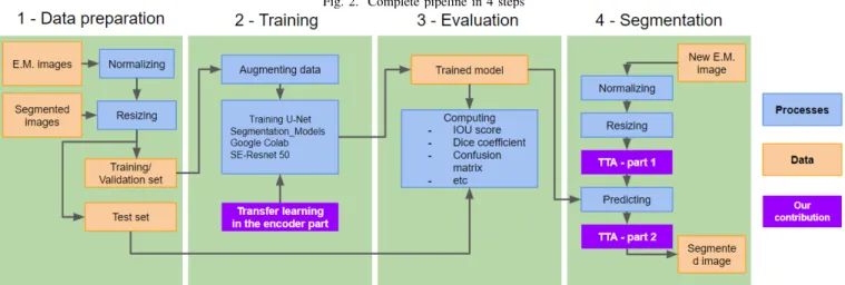
We present an update of the methods used to compute that segmentation via machine learning. Our model is based on the architecture of the U-Net network. Our main contribution consists in using transfer learning in the encoder part of the U-Net network, as well as test time augmentation when segmenting. We use the SE-Resnet50 backbone weights which was pre-trained on the ImageNet 2012 dataset.
We used a data set of 23 images with the corresponding segmented masks, which also was challenging due to its extremely small size. The results show very encouraging performances compared to the state-of-the-art with an average precision of 92% on the test images. It is also important to note that the available samples were taken from elderly mices in the corpus callosum. This represented an additional difficulty, compared to related works that had samples taken from the spinal cord or the optic nerve of healthy individuals, with better contours and less debris.
Index Terms—deep learning, segmentation, myelin, axon, g-ratio, convolutional neural network (CNN), electron microscopy
I. INTRODUCTION
In the central nervous system, white matter consists of myelinated and unmyelinated axons that connect different brain regions. Myelinated axons are wrapped by multiple layers of myelin lamellae which are tightly sealed to the axon. The myelin sheath exhibits periodic small gaps, the Nodes of Ranvier, where the axon is unmyelinated. The primary function of myelin is to speed the propagation of action potentials along the axon of a neuron by preventing the leakage of current below the myelin sheath and restricting the propagation of action potentials from one node of Ranvier to another. The axon and its associated myelin sheath are also metabolically coupled; the myelin sheath provides trophic support to the axon needed for its long-term integrity and survival [1]. The white matter has been recognized for its importance to
brain health due to the devastating effect of white matter diseases such as sclerosis, leukodystrophies or small vessel diseases of the brain. Moreover, recent works indicate that white matter can exhibit learning-dependent plasticity with formation of new myelin or changes in myelin thickness [2]. The myelin g-ratio is a quantitative measure of the relative thickness of the myelin sheath and as such a critical parameter in white matter study. It is defined as the ratio of the inner axonal diameter to the outer radius of the myelin sheath wrapped around the axon. Studies that measure the g-ratio ex vivo in the CNS typically use electron microscopy. The optimal g-ratio, to achieve maximal efficiency, is roughly comprised between 0.6-0.8. Its computation requires a robust and precise segmentation.
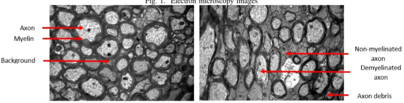
Through this article, we present the related works as well as the method we propose for segmenting these electron microscopy images in three classes : axon, myelin and back-ground (Fig. 1, left). It was an exciting challenge because working with images so hard to read (Fig. 1, right) in such a small dataset is a big feat. However, by presenting the results and compare them to the state of the art, we demonstrate that our model, based on the U-Net architecture to which we add transfer learning approaches, provides very encouraging and promising results.
II. RELATED WORKS
Segmenting axons and myelin sheaths has been a challenge for several years. First works proposed traditional image segmentation methods, favoring unsupervised approaches.
Researchers from the university of Laval, Quebec, Canada, sought to tackle this challenge in 2014 [3]. They used an unsupervised approach of boundary detection and watershed: first segmenting the axons, and then the myelin surrounding each of them. The final goal of this approach is to produce the histogram of g-ratio versus the axon equivalent diameter. This approach of segmenting axons and myelin in two parts allows for this calculation.
Fig. 1. Electron microscopy images
Another work was precedently done by AxonSeg [4], with similar methods, dataset and results. The segmentation of axons is based on the detection and analyis of local regional minima, morpholgical operations, feature extraction and dis-criminant analysis. The outer border of the myelin sheaths is obtained through minimal path and active contour algorithms. Our results will be compared to theirs towards the end of the article.V
The main issue, in the context of this problem, is the lack of generalization. This set of techniques might work out fine and give out satisfactory results on an image of good quality with normal axons and myelin sheaths, but it may fail when the image is more complex, or acquired from a sick or elderly subject. The aim of our article is to be able to treat more complex images with higher accuracy.
More recent approaches rely on deep-learning methods. CNNs have proven to be very effective in computer vision, and U-net architectures [5] have achieved very good performances in the segmentation of medical images. The first to use CNNs for myelin and axon segmentation were Mesbah et al. [6]. They did so in two main paths: the encoder-decoder architecture outperformed the per pixel approach.
Another framework developped in 2018 by Zaimi et al, called AxonDeepSeg or ADS [7] aims to answer the same problem. The authors worked with scanning electron microscopy images (SEM) and transmission electron microscopy (TEM) images. They used multiple resolutions of images, in order to improve generalization, and then manually segmented them. They pro-duced images at multiple resolutions to train a custom U-Net model and achieved the best results so far. They concluded that the use of transfer learning as well as combining multiple models would be great steps to improve both the accuracy and the robustness of the model.
III. MATERIAL
Animal experiments were conducted in full accordance with the guidelines of our local institutional Animal Care and Use Committee (Lariboisire-Villemin, CEA9). A mouse model of cerebral autosomal dominant arteriopathy with sub-cortical infarcts and leukoencephalopathy (CADASIL), Notch3R169C, and relevant controls, non-transgenic and Tg-Notch3WT mice, were used at ages 6 months and 15 months. Brains were perfusion fixed, and the anterior corpus callosum was extracted and frozen using a high pressure freezing
machine. Freeze substitution was carried out using a Leica EM AFS machine by modifying a previously used protocol (Weil et al., 2017), and brains were embedded in Epon. 70nm ultrathin sections were mounted on copper-palladium grids and stained. Images were taken using a Tecnai Spirit transmission electron microscope at 6500x (pixel size: 5.96nm; image size: 7.97x5.29m).
The dataset consists of 23 electron microscropy images, of dimensions 1336 by 888 pixels. The images are in gray levels, coded on 2 bytes. All images were segmented by an expert, who delineated manually the boundaries of the axons and myelin sheaths with a stylus. This was a very tedious task, with ambiguous parts: especially the so-called ”inner tongues”, which are not strictly myelin or axon, and unmyelinated axons difficult to identify. Our data set is also complex because the imaged samples come from pathological states, resulting in a high level of structural variability: the thickness of the myelin can vary from a few nm to a few um; the number of axons with myelin can range from 20% to 80%; the size of the ”inner tongue” can also vary considerably. We also can observe blur in some images, as well as uneven illumination. All these characteristics make the segmentation task very delicate, whether manually or automatically. Our aim is to achieve a good robustness and accuracy, despite all these features and the small size of our dataset.
Fig. 1 shows two pre-processed images. While the myelin on the first image (Fig. 1, left) is rather well-defined, it is not the case for the second one (Fig. 1, right). Not only is it much more blurry and vague, but there are a lot of debris in the background that resemble the shape and size of axons. The axons in the second image also have more complex shapes than the round ones in the first.
IV. METHODS
A. Dataset preparation
In an effort to improve generalization, we normalized our images in Matlab using the Imadjust function. We then split the dataset into 3 categories (Fig. 2): train, validation and test sets. The training set consists of 17 .tif images, the validation set of 3 and the test set of 2.
B. U-Net choice
The neural network we used to segment these electron microscopy images is based on the Net architecture [5]. U-Net is a CNN specifically developed for the segmentation of
Fig. 2. Complete pipeline in 4 steps
biomedical images. This architecture is composed of two paths giving it this U shape. The first path is the contraction path, also called encoder. It is a convolution neural network used to extract the characteristics and capture the context of the image, by computing highlevel features. The other part of the network is the expansive path, symmetrical to the contractive path, also called decoder. It consists of a sequence of upconvolutions and ascending concatenations that allows the image to be reconstructed, this time segmented, by capturing the precise localization information of the image. It is therefore an end-to-end fully convolutional network (FCN) [8]. One of the main strength of this network is the connections between the encoder and decoder parts. Those connections are used to skip features from the contracting path to the expanding path in order to recover spatial information lost during down-sampling.
C. Transfer learning
Our main contribution is the use of Transfer Learning [9] approaches in addition to the standard U-Net architecture (Fig. 2). Transfer Learning focuses on using stored knowledge, the network weights, gained while solving one problem and applying it to a different but related problem. We used the SE-Resnet50 [10] model, which is pre-trained on ImageNet dataset and fine-tuned to make it fit with our small dataset of electron microscopy images. We started by removing the model’s original classifier, then we added a new classifier that best fits our purpose. Finally, to fine-tune the model, we have frozen the convolutional base and used its outputs to feed the classifier; the pre-trained model is used as a fixed feature extraction mechanism. We implement our methods in Keras thanks to the Segmentation Model API [11]. We used the weights trained on the ImageNet 2012 dataset, provided by Segmentation Model.
D. Data augmentation
We used data augmentation [12] on the inputs of the model in order to reduce over-fitting and improve generalization and robustness (Fig 2). All the transformations have been applied
by using Albumentations [13], a fast augmentation library. Considering the context and scale of these images, we chose the following parameters and their values are summarized in table I.
TABLE I
DATA AUGMENTATION PARAMETERS
Parameter Description
Flip Randomly flips vertically and horizontally with prob-ability of 0.5
Shift Randomly shifts the image up to 10% to any direc-tion with probability of 1
Rotate Rotates the image 360 with probability of 1 Scale Scales the image up to half or double its size with a
probability 1
Perspective Changes the perspective with a probability 0.5 Brightness Changes the brightness with a probability of 0.9 Gaussian noise Adds statistical noise with a probability of 0.2 Contrast Changes the contrast with a probability of 0.45 Hue saturation Changes the color partitions with a probability of
0.45
CLAHE Updates the histogram with a probability of 0.45 Gamma Changes the gamma profile with a probability of 0.45
E. Training parameters
We performed more than fifty tests with different sets of hyper-parameters to evaluate their influence on the training and validation test. Once the model and the hyper parameters were optimized we applied it to the test images. We thus manually performed a method similar to the grid search [14]. The table II summarizes the best set of hyper-parameters.
Several hyper-parameters have a considerable influence on the performances. Among them, the use of batch normalization [15] [16] layers between the convolution and activation layers of the decoder, the learning rate which controls how much you adjust the weights of your network, the cost function and the optimizer, that govern the way in which the model achieves learning. Last but no least, the backbone which differentiates us from the others existing methods, especially from AxonDeepSeg. Indeed, we have not used the original U-Net encoder part but we have used the SE-Resnet50 model
TABLE II HYPER-PARAMETERS
Hyper-parameters Value Input size 448*672 Epochs 100 Activation function Softmax Batch size 3 Batch normalization TRUE Learning rate 0.0001 Backbone SE-Resnet50 Encoder weights ImageNet Loss Dice Loss Optimizer Nadam
thanks to transfer learning approaches. This model has been chosen by using grid searches as well.
The best results have been obtained with the use of the dice loss function and the Nadam optimizer. The loss is computed for a whole batch during the training : Eq. 1,
L(Y, ˆY ) = 1 − 2 Y ∩ ˆY |Y | + ˆ Y (1)
where Y and ˆY are respectively the ground-truth and the predicted output maps. This training phase has been executed on the Google Collab cloud platform and took only a few minutes on the NVIDIA TESLA K80 GPU provided.
F. Test time augmentation
As the model was very fast and we did not have time limitations, we chose to do test time augmentation (TTA) (Fig. 2). It is a quite uncommon method of improving the accuracy of the model. After flipping the same image, or applying the same deformations as in the data augmentation, these images are then segmented, and finally assembled together.
Our program takes an image as input, flips it vertically and horizontally. It then segments the resulting images separately using the same model, and flips them back so that they all have the same orientation. Each image ”votes” for the color of a pixel ; the stemming image’s ( of same dimensions ) accuracy is improved by around 1%. It aims to removes biases that could have grown in the treatment of verticality of the image.
G. Evaluation method
After the training, we evaluated our model on the two test images. The numerical results are presented in the results part V-B.
1) Confusion matrix: As the segmented images of the test set and the masks have the same dimensions, we were able to create a confusion matrix V-B1.
2) Precision: Precision (Eq. 2) effectively describes the purity of our positive detections relative to the ground truth.
[P recision(T P, F P ) = T P
T P + F P] (2)
3) Recall: Recall (Eq. 3) effectively describes the com-pleteness of our positive predictions relative to the ground truth.
[Recall(T P ) = T P
T P + F N] (3) 4) Dice coefficient: The Dice coefficient (Eq. 4), also known as F1-score is a metric used to gauge the similarity between the ground truth and the predicted output.
[DiceScore(T P, F P, F N ) = 2 ∗ T P
2 ∗ T P + F P + F N] (4) V. RESULTS AND DISCUSSION
A. Qualitative results
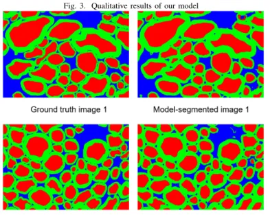
Below are the images (Fig. 3) that compose our test set, after passing through the model.
Fig. 3. Qualitative results of our model
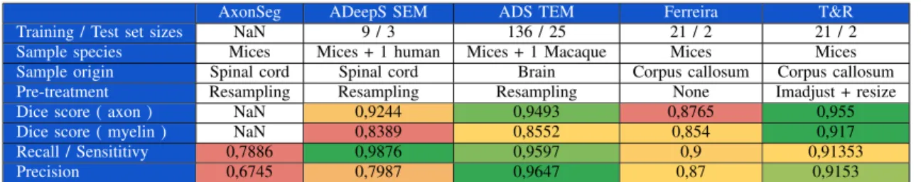
TABLE III COMPARISON OF RESULTS
AxonSeg ADeepS SEM ADS TEM Ferreira T&R Training / Test set sizes NaN 9 / 3 136 / 25 21 / 2 21 / 2
Sample species Mices Mices + 1 human Mices + 1 Macaque Mices Mices
Sample origin Spinal cord Spinal cord Brain Corpus callosum Corpus callosum
Pre-treatment Resampling Resampling Resampling None Imadjust + resize
Dice score ( axon ) NaN 0,9244 0,9493 0,8765 0,955
Dice score ( myelin ) NaN 0,8389 0,8552 0,854 0,917
Recall / Sensititivy 0,7886 0,9876 0,9597 0,9 0,91353
Precision 0,6745 0,7987 0,9647 0,87 0,9153
We identified 4 classes of errors, in which the other visible ones can be associated with. Error 1 can is linked to the dark nucleus of the axon, which is detected as background. Training the model on more axons with nuclei or tuning these spots down in pre-processing could solve this issue.
Error 2 can be attributed to the extreme shape of the axon. Very elongated, the model chooses to split it in two. These odd shapes are rare in the dataset ; training the model with more diverse profiles of axons could help with generalization. Error 3 can be attributed to myelin debris or noise in the image. This particular method of obtaining the image leaves room for some indistinguishable parts.
Error 4 is actually due to the fact that axon debris are present. They are hard to distinguish from background, but could be relevant for computing the g-ratio.
Even though the contours of the myelin sheaths are matching the one of the segmented image, the distinction between each individual myelin sheath is not made.
B. Quantitative results
1) Confusion matrix: We obtained this table by computing the difference by pixel in the starting and final images. We then averaged the results between test images, and scaled them to 100%.
The true positives are in majority, but there is a net distinction between the three classes. Myelin contour is hard to define, and as previously mentioned, there are some structures in the image that are very ambiguous, and even an expert has difficulty to know wether it is an axon or not. The posteriori qualitative analysis of the segmentations showed that some axons were rightly segmented although they were not in the ground truth. Dr Joutel also identified myelin debris that were not manually segmented.
TABLE IV
CONFUSION MATRIX PRE AND POST-TTA in %
(Pre - Post TTA)
Model segmentation Axon Myelin Other Ground
truth
Axon 79.1 - 80.3 19.4 - 19.3 1.5 - 0.4 Myelin 14.9 - 15.0 58.0 - 58.5 27.1 - 26.5
Other 19.7 - 19.4 23.7 - 24.4 56.6 - 56.2
2) Metrics results: For each metric, we computed the score obtained on each class separately, doing a pixel-by-pixel analysis. We finally compute the average of these scores for the two test images. Using TTA slightly improved an already
well-performing model.
We can see that the scores computed on the axon class are the best, slightly ahead of those calculated on the myelin class. On the other hand, the results of the scores computed on the background class are much worse. We can interpret these results as follow: the axons are well segmented while the myelin is more difficult to circumvent and sometimes spills over into the background or the axons. Finally, the less good scores of the background class are due to the fact that the model sometimes finds axons and myelin which are not segmented on the ground truth image. Paradoxically, this bad score partly reflects the strength of our model. The results obtained are presented in the table V. It is also interesting to compare the time it takes to process a full image. The AxonSeg technique takes around 8 hours to segment a 110000 axon images, while ours segments images of same axon density in around 7 minutes.
TABLE V METRICS RESULTS
Axon Myelin Background Recall 0,946 0,941 0,827 Precision 0,963 0,894 0,911 Dice score 0,955 0,917 0,867
3) Performance comparison: Table V presents the compari-son of our performance with other similar works. ADS stands for AxonDeepSeg, which is the reference algorithm in this field. It is worth noting that the data sets are different, ours being much more challenging because of the extremely small dataset and the high image variability.
We originally tried to use the same architecture and techniques as AxonDeepSeg, in order to optimise furthermore the hyper-parameters of their model. These results can be seen in the ”Ferreira” column, by the name of the student who used this method. This approach did not bear great fruits, as our dataset was much smaller, but this first step was necessary.
Our final results, labelled ”Our model”, compete with the ones of AxonDeepSeg. Even though the size of the dataset has a strong influence on the results obtained, we can achieve slightly better dice scores. Moreover, the designers of ADS trained their model and tested it on electron microscopy images taken from young and healthy animals. In our case, we were dealing with older mices which represents an additional difficulty on the segmentation of the images. Finally, ADS
images are taken from the spinal cord while ours are taken from the corpus callosum where segmentation is more difficult to perform.
VI. CONCLUSION AND PERSPECTIVES
Using transfer learning and test time augmentation, paired via the standard hyper-parameters optimization techniques only betters the outcome of the model. Taking the most steps possible in order to improve the generalization of the model is important as well, and we tried our best at it. This also was an exercise of working with a rather extreme dataset. The total number of training images and their definition was very low, and the quality of the myelin in some cases was challenging. The Hausdorff Distance is widely used in evaluating medi-cal image segmentation methods. Using this boundary-based metric could improve the qualitative results of the predictions. One could build on the work described in [17].
Moreover, we could see that increasing the size of the dataset had a favourable impact on the quantitative results obtained. This avenue will soon be explored because the Paris Lari-boisire hospital will provide us additional images.
We also consider adversarial normalization as a possible improvement [18]. There exist many ways of collecting these images, and there might exist disparities within a same image: adapting the normalization to the dataset could improve the robustness of the model further more.
The ultimate goal of this segmentation tool would be to then compute the g-ratio of each axon. Computing the g-ratio for every axon will enable us to get a very reliable histogram, which is valuable to characterize diseases affecting the white matter.
VII. ACKNOWLEDGEMENTS
We would like to thank all the authors who contributed to the writing of this paper, as well as Stephanie Ferreira who has previously worked on the subject (cf. III and V-B3).
REFERENCES
[1] Christine Stadelmann, Sebastian Timmler, Alonso Barrantes-Freer, and Mikael Simons. Myelin in the cen-tral nervous system: structure, function, and pathology. Physiological reviews, 99(3):1381–1431, 2019.
[2] Cassandra Sampaio-Baptista and Heidi Johansen-Berg. White matter plasticity in the adult brain. Neuron, 96(6):1239–1251, 2017.
[3] Steve B´egin, Olivier Dupont-Therrien, Erik B´elanger, Amy Daradich, Sophie Laffray, Yves De Koninck, and Daniel C Cˆot´e. Automated method for the segmentation and morphometry of nerve fibers in large-scale cars images of spinal cord tissue. Biomedical optics express, 5(12):4145, 2014.
[4] Aldo Zaimi, Tanguy Duval, Alicja Gasecka, Daniel Cˆot´e, Nikola Stikov, and Julien Cohen-Adad. Axonseg: open source software for axon and myelin segmentation and morphometric analysis. Frontiers in neuroinformatics, 10:37, 2016.
[5] Olaf Ronneberger, Philipp Fischer, and Thomas Brox. U-net: Convolutional networks for biomedical image segmentation. In International Conference on Medical image computing and computer-assisted intervention, pages 234–241. Springer, 2015.
[6] Rassoul Mesbah, Brendan McCane, and Steven Mills. Deep convolutional encoder-decoder for myelin and axon segmentation. In 2016 International Conference on Image and Vision Computing New Zealand (IVCNZ), pages 1–6. IEEE, 2016.
[7] Aldo Zaimi, Maxime Wabartha, Victor Herman, Pierre-Louis Antonsanti, Christian S Perone, and Julien Cohen-Adad. Axondeepseg: automatic axon and myelin segmen-tation from microscopy data using convolutional neural networks. Scientific reports, 8(1):1–11, 2018.
[8] Jonathan Long, Evan Shelhamer, and Trevor Darrell. Fully convolutional networks for semantic segmentation. In Proceedings of the IEEE conference on computer vision and pattern recognition, pages 3431–3440, 2015. [9] Annegreet Van Opbroek, M Arfan Ikram, Meike W Vernooij, and Marleen De Bruijne. Transfer learning improves supervised image segmentation across imag-ing protocols. IEEE transactions on medical imagimag-ing, 34(5):1018–1030, 2014.
[10] Jie Hu, Li Shen, and Gang Sun. Squeeze-and-excitation networks. In Proceedings of the IEEE conference on computer vision and pattern recognition, pages 7132– 7141, 2018.
[11] Pavel Yakubovskiy. Segmentation models. https://github. com/qubvel/segmentation models, 2019.
[12] Luis Perez and Jason Wang. The effectiveness of data augmentation in image classification using deep learning. arXiv preprint arXiv:1712.04621, 2017.
[13] Alexander Buslaev, Vladimir I. Iglovikov, Eugene Khvedchenya, Alex Parinov, Mikhail Druzhinin, and Alexandr A. Kalinin. Albumentations: Fast and flexible image augmentations. Information, 11(2), 2020. [14] James Bergstra and Yoshua Bengio. Random search
for hyper-parameter optimization. Journal of machine learning research, 13(Feb):281–305, 2012.
[15] Shibani Santurkar, Dimitris Tsipras, Andrew Ilyas, and Aleksander Madry. How does batch normalization help optimization? In Advances in Neural Information Pro-cessing Systems, pages 2483–2493, 2018.
[16] Sergey Ioffe and Christian Szegedy. Batch normalization: Accelerating deep network training by reducing internal covariate shift. arXiv preprint arXiv:1502.03167, 2015. [17] Davood Karimi and Septimiu E Salcudean. Reducing
the hausdorff distance in medical image segmentation with convolutional neural networks. IEEE transactions on medical imaging, 2019.
[18] Pierre-Luc Delisle, Benoit Anctil-Robitaille, Christian Desrosiers, and Herve Lombaert. Adversarial normaliza-tion for multi domain image segmentanormaliza-tion. arXiv preprint arXiv:1912.00993, 2019.