HAL Id: hal-01790282
https://hal.archives-ouvertes.fr/hal-01790282
Submitted on 11 May 2018
HAL is a multi-disciplinary open access
archive for the deposit and dissemination of
sci-entific research documents, whether they are
pub-lished or not. The documents may come from
teaching and research institutions in France or
abroad, or from public or private research centers.
L’archive ouverte pluridisciplinaire HAL, est
destinée au dépôt et à la diffusion de documents
scientifiques de niveau recherche, publiés ou non,
émanant des établissements d’enseignement et de
recherche français ou étrangers, des laboratoires
publics ou privés.
Improving the AODV-based ZigBee Routing Protocol
through Pivots
Nancy Rachkidy, Alexandre Guitton, Chiara Buratti
To cite this version:
Nancy Rachkidy, Alexandre Guitton, Chiara Buratti. Improving the AODV-based ZigBee Routing
Protocol through Pivots. PIMRC (IEEE International Symposium on Personal, Indoor and Mobile
Radio Communications), 2013, London, United Kingdom. �hal-01790282�
Improving the AODV-based ZigBee Routing
Protocol through Pivots
Nancy El Rachkidy
∗, Alexandre Guitton
∗, Chiara Buratti
†∗ Clermont Universit´e, Universit´e Blaise Pascal, LIMOS
BP 10448, F-63000 Clermont-Ferrand CNRS, UMR 6158, LIMOS, F-63173 Aubi`ere Email:{nancy,guitton}@sancy.univ-bpclermont.fr
† DEI, University of Bologna
Email: [email protected]
Abstract—Wireless sensor networks are often deployed for
monitoring purposes: when nodes detect the occurrence of a significant event, they transmit an information to a control entity in a multi-hop fashion. When data rate increases, congestion becomes a fundamental issue, especially when an emergency situation generates alarm messages originating from a specific area of the network. Indeed, congestion increases delays and packet losses, and yields to an unfair use of the energy of nodes. In this paper, we propose to improve the ZigBee routing protocol, aiming at reducing traffic congestion. The proposed solution uses intermediate nodes, denoted as pivots, which are selected by the data sources in order to reduce congestion on paths. Simulation results highlight the significant improvement achieved in terms of packet losses and average delays, with respect to the ZigBee routing protocol, while the overhead generated in the network is maintained under control. A mathematical model to derive the average path length and the number of pivots is also provided.
I. INTRODUCTION
Environmental monitoring generally requires the deploy-ment of a wireless sensor network (WSN), where nodes are low-cost devices, interconnected through wireless links, and supplied by a limited amount of initial energy. Nodes sense the physical environment and transmit the measurement results to a control entity, called the sink. In typical monitoring applications, the WSN is deployed over a large area; once an event occurs (e.g., a fire in a forest), nodes detecting the event become to send data toward the sink.
IEEE 802.15.4 [1] is considered the standard de-facto for WSNs: it describes a short-range wireless technology intended for applications with relaxed throughput and latency require-ments. IEEE 802.15.4 specifies the physical (PHY) layer and medium access control (MAC) layer protocol, while the ZigBee [2] standard describes the upper layers protocols of an IEEE 802.15.4-compliant network. ZigBee defines a network layer capable of peer-to-peer multi-hop mesh networking, and an application layer for interoperable application profiles. ZigBee defines two routing protocols: a tree-based routing, and an Ad-hoc On-demand Distance Vector (AODV)-based routing [3], [4], [5]. The tree-based routing is simple and does not require to store routing tables in devices, but has two major drawbacks: first, it yields to long paths (in terms of hop count) as it is not based on shortest paths (unlike AODV); second, nodes that are close to the root of the tree (which is also the
node coordinating the ZigBee network) consume more power than the others, because nodes close to the root must handle the traffic of the lower levels nodes.
In this paper, we focus on the AODV-based ZigBee routing protocol, which is suitable for large WSNs. We propose an improvement of this protocol in order to reduce traffic con-gestion. In data networking and queueing theory, congestion occurs whenever a link carries more data than it can handle, causing a deterioration of its quality [6]. Typical effects of congestion include an increase of queueing delays and packet losses, and an unfair use of the energy resources of nodes in the network (as the most used routers consume more energy), which shortens network lifetime. The main reason of traffic congestion in ZigBee is that paths are selected according to connectivity and hop count, without considering the level of interference on the links: we aim to improve the AODV-based ZigBee routing protocol by forcing paths to slightly differ from those obtained by AODV, by using intermediate nodes called pivots. The proposed solution allows to improve the performance, without increasing significantly the overhead generated in the network. A mathematical model to derive the average number of pivots for a given source and the average path length is also presented. Comparisons between mathematical model and simulations show the impact of the transmission of control packets on the discovery of pivots, as these control packets are implemented in the simulator but not accounted for in the model, where only the rules for selecting pivots are considered. The mathematical model is also an useful tool to improve the pivot selection mechanism and reduce the overhead.
The remainder of the paper is the following. In Sect. II related works are reported. Sect. III provides some details about the IEEE 802.15.4 and ZigBee standards. Sect. IV describes our proposition based on pivots and provides the mathematically model. Sect. V presents our simulation set-tings, and compares the performance of our approach with respect to the AODV-based ZigBee routing protocol, using simulations. Finally, Sect. VI concludes our work.
II. RELATED WORKS
Many works focus on improving the AODV-based ZigBee routing protocol. In [7], the AODV-based ZigBee routing protocol is modified to decrease the retransmission of flooding packets in order to make routing more efficient and to avoid the broadcasting storm problem. Nodes are grouped into logical clusters, and nodes in the same clusters share a routing table, which reduces the number of RREQ packets that are broadcasted. In [8], the authors present a multipath energy aware AODV routing, where the topology is divided into logical clusters. The flooding of RREQ packets is restricted to nodes outside the cluster, in order to reduce the overhead of the route discovery. In this paper, we aim at changing the paths that AODV builds, rather than optimizing the way AODV builds the paths.
Pivot-based routing introduces diversity in routing: packets are sent from sources to pivots, and from pivots to destinations. In [9], the author proposes a centralized approach where 𝑘 paths are built from the source to the destination. Each path goes through several pivots, and the distance between pivots is limited by a threshold. The algorithm requires a global knowledge of the network, unlike our approach which is distributed (and which focuses on the case 𝑘 = 1, with one pivot only on the path). In [10], the authors propose a pivot routing protocol which aims to reduce the control message overhead and extend the network lifetime. In order to select pivot, the sink propagates a query and selects candidate nodes as pivots based on the distance (for instance). A node is candidate if its distance from the sink (or from a previous pivot) exceeds a threshold. Each node maintains a return path to the previous pivot (or sink). In addition, several paths can be maintained between pivots. In our approach, we use only one pivot per path, and our objective is to select pivots so that paths from sources to destinations do not overlap and do not cause congestion. In [11], we proposed a pivot-based protocol for a tree-based network in order to avoid congestion when several sources send data to the same destination. The differences with this paper are the following: we now focus on AODV-based routing rather than on the hierarchical routing, and we have changed the rules to select pivots in order to deal with an ad-hoc routing protocol.
III. IEEE 802.15.4ANDZIGBEE STANDARDS
IEEE 802.15.4 [1] defines two operational modes, namely beacon-enabled and non beacon-enabled. In this paper we consider the non beacon-enabled mode, where the medium access mechanism is a Carrier-Sense Multiple Access with Collision Avoidance (CSMA/CA) algorithm, called Unslotted CSMA/CA. In Unslotted CSMA/CA, losses may occur due to hidden terminals.
In the AODV-based ZigBee routing protocol [2], each link 𝑙𝑖 is characterized by a link cost𝐶𝑙𝑖, such that
𝐶𝑙𝑖 = min{7, ⌊𝑃𝑙−4𝑖 ⌋} , (1)
where 𝑃𝑙𝑖 is the probability of packet delivery on the link 𝑙𝑖. To establish a path between a source and a destination,
the protocol selects the path 𝑃 = (𝑙1, 𝑙2, . . . , 𝑙𝐿), where 𝐿 is
the path lenght, having the smallest total cost, 𝐶(𝑃 ), where
𝐶(𝑃 ) =∑𝐿𝑖=1𝐶𝑙𝑖. If there are several paths having the same
cost, the shortest path among them (in terms of hop count) is chosen.
The AODV-based ZigBee routing protocol computes routes in the following way. The source node start broadcasting a route request (RREQ) packet. When intermediate nodes receive the RREQ, they record the address of the sender and the link cost (where𝑃𝑙𝑖depends on the link quality with which
the RREQ was received) in a route discovery table. If the cost of the path using this link is better that the cost of the previous path in the table, the intermediate node rebroadcasts the RREQ to its neighbors. When the destination node receives the RREQ, it responds by unicasting a route reply (RREP) packet back to its neighbor from which it received the RREQ. RREPs are routed back to the source node using the route discovery table, and route entries are set up as the RREP progresses. Note that RREQ packets are sent without Unslotted CSMA/CA, but with a random jitter uniformly distributed within a given range, and that RREPs are sent with Unslotted CSMA/CA and with acknowledgments.
IV. PROPOSITION
We consider nodes distributed on a grid1 (see Fig. 1), and an event-driven application, such that once an event happens, nodes detecting it start sending data to a final sink.
In the following, we detail a mechanism that selects pivots in order to improve the AODV-based ZigBee routing protocol. Then, we describe a mathematical model of our pivot selection. A. Proposed pivot selection mechanism
Let 𝑆 be a source node and 𝐷 be a destination node. We
assume nodes know their positions in the grid. A node𝑃 is a potential pivot for the pair (𝑆, 𝐷) if it satisfies the following criteria:
1) 𝑃 is not located on the shortest path from 𝑆 to 𝐷,
2) 𝑃 is closer to the destination 𝐷 than to the source 𝑆,
3) 𝑃 is located within the virtual rectangle having 𝑆 and
𝐷 as diagonally opposite angles.
The first rule ensures that the path from 𝑆 to 𝑃 is divergent from the path from 𝑆 to 𝐷. In this way, if there are several sources nearby, we can expect the paths from sources to pivots to present diversity. The second rule ensures that the path from 𝑃 to 𝐷 does not converge to 𝐷 too early (which would cancel the benefits of the first rule). The third rule ensures that the data path (through the pivot) is not too long.
By denoting as 𝑑(𝐴, 𝐵) the distance in number of hops between node𝐴 and 𝐵, a node in position (𝑥, 𝑦) is a potential pivot for a pair(𝑆, 𝐷) in locations (𝑥𝑆, 𝑦𝑆) and (𝑥𝐷, 𝑦𝐷) only if (according to the three rules stated above):
1) 𝑑(𝑆, 𝑃 ) + 𝑑(𝑃, 𝐷) > 𝑑(𝑆, 𝐷) + 𝜀,
2) 𝑑(𝑆, 𝑃 ) > 𝑑(𝑃, 𝐷),
1The protocol is adapted for non-grid topologies as hop-count is used as
3) min{𝑥𝑆, 𝑥𝐷} ≤ 𝑥 ≤ max{𝑥𝑆, 𝑥𝐷} and
min{𝑦𝑆, 𝑦𝐷} ≤ 𝑦 ≤ max{𝑦𝑆, 𝑦𝐷},
where 𝜀 is a threshold chosen according to the network size. Assuming a circular transmission range, and denoting the transmission range, expressed in number of hops on the grid, asℎ𝑇, we can define the distance in number if hops between two nodes𝐴 and 𝐵, being in positions (𝑥𝐴, 𝑦𝐴) and (𝑥𝐵, 𝑦𝐵),
respectively, as: 𝑑(𝐴, 𝐵) = max {⌈ ∣𝑥𝐵− 𝑥𝐴∣ ℎ𝑇 ⌉ , ⌈ ∣𝑦𝐵− 𝑦𝐴∣ ℎ𝑇 ⌉} (2) Our mechanism uses RREQs/RREPs for discovering pivots. Indeed, a RREQ is sent by each source 𝑆, including some information required for pivot discovery. All the potential pivots for𝑆 reply with a RREP. Note that due to its broadcast nature, the RREQ reaches all nodes in the network, while only potential pivots reply with the RREP. The mechanism works according to the following steps:
∙ The sink 𝐷 sends a broadcast packet (to be forwarded to all nodes in the network), containing its position (𝑥𝐷, 𝑦𝐷), such that each node 𝑁 may compute the
distance𝑑(𝑁, 𝐷);
∙ Each source𝑆 sends a RREQ, including the information about𝑑(𝑆, 𝐷) and its position (𝑥𝑆, 𝑦𝑆), for searching its
potential pivots;
∙ Each node𝑁 determines whether it is a potential pivot or not for the pair(𝑆, 𝐷) (using the three rules mentioned above, and the knowledge of𝑑(𝑆, 𝑁), 𝑑(𝑁, 𝐷), 𝑑(𝑆, 𝐷) and the positions of𝑆 and 𝐷) after having received the RREQ;
∙ If a node𝑁 is a potential pivot, it notifies 𝑆 of its role, by sending back a RREP.
At this point, each source 𝑆 selects a pivot 𝑃 among the potential pivots (in this paper the selection is random), and starts transmitting data to𝑃 using the path already established. The pivot 𝑃 then sends a RREQ to 𝐷 and waits the RREP
from𝐷 in order to start transmitting data to 𝐷. If there is no
pivot for a pair(𝑆, 𝐷), the node 𝐷 itself is used as a pivot. B. Mathematical model
To simplify, we assume that the source node is below and on the left of the destination node, that is 𝑥𝑆 < 𝑥𝐷 and
𝑦𝑆 < 𝑦𝐷. The other cases could be obtained by symmetry.
We also assume that no channel fluctuation are present, therefore we can define a transmission range, denoted as 𝑟𝑇. We mathematically compute 𝑛pivot, which is the number of
potential pivots in the network for a given source, and 𝑙pivot,
which is the average path length connecting the source to the destination via the pivot, expressed in number of hops.
A node in location (𝑥, 𝑦) is a potential pivot for a pair (𝑆, 𝐷) in locations (𝑥𝑆, 𝑦𝑆) and (𝑥𝐷, 𝑦𝐷) if 𝑥𝑆 ≤ 𝑥 ≤ 𝑥𝐷
and𝑦𝑆 ≤ 𝑦 ≤ 𝑦𝐷 (which refers to rule number 3) and if the
following conditions are satisfied: 1) max {⌈ 𝑥−𝑥𝑆 ℎ𝑇 ⌉ ,⌈𝑦−𝑦𝑆 ℎ𝑇 ⌉} + max{⌈𝑥𝐷−𝑥 ℎ𝑇 ⌉ ,⌈𝑦𝐷−𝑦 ℎ𝑇 ⌉} > max{⌈𝑥𝐷−𝑥𝑆 ℎ𝑇 ⌉ ,⌈𝑦𝐷−𝑦𝑆 ℎ𝑇 ⌉} + 𝜀 2) max {⌈ 𝑥−𝑥𝑆 ℎ𝑇 ⌉ ,⌈𝑦−𝑦𝑆 ℎ𝑇 ⌉} > max{⌈𝑥𝐷−𝑥 ℎ𝑇 ⌉ ,⌈𝑦𝐷−𝑦 ℎ𝑇 ⌉} expressing rules number 1 and 2, respectively. In the following, for the sake of legibility of formulas, we set𝑥𝑆𝑃 =
⌈ 𝑥−𝑥𝑆 ℎ𝑇 ⌉ , 𝑦𝑆𝑃 = ⌈ 𝑦−𝑦𝑆 ℎ𝑇 ⌉ , 𝑥𝑃 𝐷 = ⌈ 𝑥𝐷−𝑥 ℎ𝑇 ⌉ , 𝑦𝑃 𝐷 = ⌈ 𝑦𝐷−𝑦 ℎ𝑇 ⌉ , 𝑥𝑆𝐷 = ⌈ 𝑥𝐷−𝑥𝑆 ℎ𝑇 ⌉ , and𝑦𝑆𝐷= ⌈ 𝑦𝐷−𝑦𝑆 ℎ𝑇 ⌉ .
The system of equations defined above has solutions (dif-ferent from zero), only in the following four cases:
1) 𝑥𝑆𝑃 ≥ 𝑦𝑆𝑃,𝑥𝑃 𝐷< 𝑦𝑃 𝐷 and𝑥𝑆𝐷≥ 𝑦𝑆𝐷. The system
becomes𝑥𝑆𝑃 > 𝑦𝑃 𝐷 and𝑥𝑆𝑃+ 𝑦𝑃 𝐷> 𝑥𝑆𝐷+ 𝜀.
2) 𝑥𝑆𝑃 ≥ 𝑦𝑆𝑃,𝑥𝑃 𝐷< 𝑦𝑃 𝐷 and𝑥𝑆𝐷< 𝑦𝑆𝐷. The system
becomes𝑥𝑆𝑃 > 𝑦𝑃 𝐷 and𝑥𝑆𝑃+ 𝑦𝑃 𝐷> 𝑦𝑆𝐷+ 𝜀.
3) 𝑥𝑆𝑃 < 𝑦𝑆𝑃,𝑥𝑃 𝐷≥ 𝑦𝑃 𝐷 and𝑥𝑆𝐷≥ 𝑦𝑆𝐷. The system
becomes𝑦𝑆𝑃 > 𝑥𝑃 𝐷 and𝑦𝑆𝑃 + 𝑥𝑃 𝐷> 𝑥𝑆𝐷+ 𝜀.
4) 𝑥𝑆𝑃 < 𝑦𝑆𝑃,𝑥𝑃 𝐷≥ 𝑦𝑃 𝐷 and𝑥𝑆𝐷< 𝑦𝑆𝐷. The system
becomes𝑦𝑆𝑃 > 𝑥𝑃 𝐷 and𝑦𝑆𝑃 + 𝑥𝑃 𝐷> 𝑦𝑆𝐷+ 𝜀. Our first metric 𝑛pivot can be defined as:
𝑛pivot= 𝑦𝐷 ∑ 𝑦=𝑦𝑆 𝑥𝐷 ∑ 𝑥=𝑥𝑆 𝑓(𝑥, 𝑦), (3)
where𝑓(𝑥, 𝑦) is 0 if the node at location (𝑥, 𝑦) is not a pivot, and 1 if it is. By merging cases 1 and 2, when 𝑥𝑆𝑃 ≥ 𝑦𝑆𝑃,
𝑥𝑃 𝐷< 𝑦𝑃 𝐷 and𝑥𝑆𝑃 > 𝑦𝑃 𝐷, we have: 𝑓(𝑥, 𝑦) = ⎧ ⎨ ⎩ 1 if (𝑥𝑆𝐷≥ 𝑦𝑆𝐷 and𝑥𝑆𝑃+ 𝑦𝑃 𝐷> 𝑥𝑆𝐷+ 𝜀) or (𝑥𝑆𝐷< 𝑦𝑆𝐷 and𝑥𝑆𝑃 + 𝑦𝑃 𝐷> 𝑦𝑆𝐷+ 𝜀) 0 otherwise. (4) By merging cases 3 and 4, when 𝑥𝑆𝑃 < 𝑦𝑆𝑃, 𝑥𝑃 𝐷 ≥ 𝑦𝑃 𝐷
and𝑦𝑆𝑃 > 𝑥𝑃 𝐷, we have: 𝑓(𝑥, 𝑦) = ⎧ ⎨ ⎩ 1 if (𝑥𝑆𝐷≥ 𝑦𝑆𝐷 and𝑦𝑆𝑃+ 𝑥𝑃 𝐷> 𝑥𝑆𝐷+ 𝜀) or (𝑥𝑆𝐷< 𝑦𝑆𝐷 and𝑦𝑆𝑃+ 𝑥𝑃 𝐷> 𝑦𝑆𝐷+ 𝜀) 0 otherwise. (5) The average length of the path connecting the source and the destination, passing through the potential pivot, and averaged over all the potential pivots, is given by:
𝑙pivot= 𝑦𝐷 ∑ 𝑦=𝑦𝑆 𝑥𝐷 ∑ 𝑥=𝑥𝑆 𝑓(𝑥, 𝑦) ⋅ [𝑑(𝑆, 𝑃𝑥,𝑦) + 𝑑(𝑃𝑥,𝑦, 𝐷)]/𝑛pivot, (6) where 𝑃𝑥,𝑦 indicates that𝑃 is in location (𝑥, 𝑦).
The above expressions can be simplified when ℎ𝑇 = 1. In particular, by setting𝑚 = 𝑥𝑆−𝑦𝑆,𝑛 = 𝑥𝐷+𝑦𝑆,𝑝 = 𝑥𝑆+𝑦𝐷, 𝑢 = 𝑥𝐷− 𝑦𝐷, ˆ𝜀 = ⌈𝜀2⌉, ˆ𝑥𝐷= ⌈𝑥2𝐷⌉, we have: ˆ𝑥𝑆 = { ⌈𝑥𝑆 2 ⌉ if 𝑥𝑆− 𝑥𝐷 is even ⌊𝑥𝑆 2 ⌋ otherwise. (7) ˆ𝑦𝐷= ⎧ ⎨ ⎩ ⌈𝑦𝐷 2 ⌉ if 𝑥𝑆− 𝑥𝐷 and𝑦𝑆− 𝑦𝐷
are both odd or both even
⌊𝑦𝐷 2 ⌋ otherwise. (8) ˆ𝑦𝑆 = { ⌊𝑦𝑆
2⌋ if 𝑥𝑆− 𝑥𝐷 is even and𝑦𝑆− 𝑦𝐷 is odd
⌈𝑦𝑆
2⌉ otherwise.
0 1 2 3 4 5 6 7 8 9 10 11 12 13 14 15 16 17 18 19 20 21 22 23 24 25 26 27 28 29 30 31 32 33 34 35 36 37 38 39 40 41 42 43 44 45 46 47 48 x y Event
Fig. 1. The reference scenario: nodes deployed in a grid.
For the case𝑥𝐷− 𝑥𝑆 ≥ 𝑦𝐷− 𝑦𝑆, we obtain: 𝑛pivot= ∑𝑦𝐷 𝑦=𝑦𝑆 ∑min{𝑦+𝑚−ˆ𝜀,𝑥𝐷} 𝑥=max{𝑛−𝑦+1,𝑥𝑆}1 +∑min{𝑦𝐷+ˆ𝑥𝑆−ˆ𝑥𝐷−ˆ𝜀,𝑦𝐷} 𝑦=𝑦𝑆 ∑𝑥𝐷 𝑥=max{𝑝−𝑦+1,𝑥𝑆} 1 +∑𝑦𝐷 𝑦=max{𝑦𝐷+𝑞−ˆ𝜀+1,𝑦𝑆} ∑𝑥𝐷 𝑥=max{𝑦+𝑢+𝜀+1,𝑥𝑆}1 (10)
For the case𝑥𝐷− 𝑥𝑆 < 𝑦𝐷− 𝑦𝑆, we have: 𝑛pivot= ∑𝑦 𝐷 𝑦=𝑦𝑆 ∑min{𝑦+𝑢−𝜀−1,𝑥 𝐷} 𝑥=max{𝑛−𝑦+1,𝑥𝑆}1 +∑min{𝑡−ˆ𝜀,𝑦𝐷} 𝑦=𝑦𝑆 ∑𝑥 𝐷 𝑥=max{𝑝−𝑦+1,𝑥𝑆}1 +∑𝑦𝐷 𝑦=max{ˆ𝑦𝐷+ˆ𝑦𝑆−ˆ𝜀+1,𝑦𝑆} ∑𝑥 𝐷 𝑥=max{𝑦+𝑚+𝜀+1,𝑥𝑆}1 (11)
Finally, note that when it is not true that the source node is below and on the left of the destination node, the above formulas are still valid, simply setting:𝑥𝑆 = min{𝑥𝑆1, 𝑥𝐷1},
𝑥𝐷 = max{𝑥𝑆1, 𝑥𝐷1}, 𝑦𝑆 = min{𝑦𝑆1, 𝑦𝐷1} and 𝑦𝐷 =
max{𝑦𝑆1, 𝑦𝐷1}, where (𝑥𝑆1, 𝑦𝑆1) and (𝑥𝐷1, 𝑦𝐷1) are the
actual locations of the source and destination. V. SIMULATION RESULTS
In this section, we first give details about our implemen-tation and scenarios. Then, we show the benefits of our mechanism according to several metrics.
A. Implementation details
We assume that the loss in dB between a transmitter and a receiver at distance 𝑑 is given by: 𝐿[dB] = 𝑘0+ 𝑘1ln 𝑑, where 𝑘0 is a function of the propagation coefficient and 𝑘1 = 10𝛽/ ln 10, where 𝛽 is a constant. The received power
in logarithmic scale, denoted as𝑃𝑅, is given by 𝑃𝑅[dBm] =
𝑃𝑇[dBm] − 𝐿[dB], where 𝑃𝑇 is the transmitted power. The physical layer of IEEE 802.15.4 uses an Offset Quadra-ture Phase Shift Keying (O-QPSK) modulation with half-sine pulse shaping. With this modulation, the bit error probability can be defined as 𝑃𝑒𝑏 = 12erfc(√𝑊 ). 𝑊 is the conventional signal-to-noise-ratio, and is given by𝑊 = 𝑃𝑅/(2 ⋅ 𝑁0⋅ 𝑅𝑏), where 𝑁0is the bilateral power spectral density of the Gaus-sian noise,𝑅𝑏 is the bit rate (which is set to 250 kbit/s as we
focus on the 2.4 GHz industrial, scientific and medical (ISM) frequency band), and erfc is the complementary error function, defined as:
erfc(𝑥) = 1 − erf(𝑥), erf(𝑥) = √2 𝜋
∫ 𝑥
0 𝑒
−𝑦2
𝑑𝑦. (12)
The packet capture model is the following. A packet is captured if 𝐶𝐼 > 𝐶𝐼∣min, where 𝐶 is the power received from
the useful signal and 𝐼 is the sum of the interfering powers. Once a packet is captured, we use probability𝑃𝑙to determine if all the bits of the packets are correct. Assuming that a packet is composed of 𝑁bit bits, we have 𝑃𝑙 = (1 − 𝑃𝑒𝑏)𝑁bit. 𝑃
𝑙 is
used in Eq. (1) to compute the link cost. B. Simulation scenarios and parameter settings
We considered the grid topology shown in Fig. 1, having 7×7 nodes, with 10 m between nodes. We set the following parameters: 𝑘0 = 40 dB, 𝛽 = 3.5, 𝐶𝐼∣min = 1.3 dB, 𝑁0 =
5 ⋅ 10−20 W/Hz (which corresponds to a receiver sensitivity
of -97 dBm). We also set 𝑃𝑇 = −15 dBm, which yields to an ideal transmission range 𝑟𝑇 of 15.85m. The size of data packets at the PHY layer is 36 bytes. The size of ACK packets is 8 bytes. RREQ and RREP packets have a size of 36 bytes. As 𝑟𝑇 is 15.85 m, nodes can communicate with the eight adjacent nodes (i.e., ℎ𝑇 = 1). Finally, we set the jitter for RREQs to be randomly chosen in the interval [0.5; 1] s.
We considered two simulation scenarios. In the first sce-nario, the event-driven application is considered, therefore sources nodes are: 0, 1, 7 and 8, while the sink is node 48. The aim of this scenario is to highlight the congested area on the shortest path from the sources to the destination. In the second scenario, sources are more distributed in the area (in particular we consider nodes 0, 6, 24 and 42), while the destination is always node 48. The aim of this scenario is to show that our mechanism still achieves good performance also when sources are more distributed in the network.
We evaluated the average packet loss, the average end-to-end delay, the average path length and the average number of control packets, for three cases: AODV-based ZigBee routing protocol (referred to as ZigBee), AODV with pivots and different values of𝜀.
We simulate 100 different repetitions, characterized by different RREQs/RREPs transmissions to search for paths and pivots (i.e., characterized by different paths), and for each repetition we transmit 1.000 packets per source. Results are averaged among the different repetitions, transmissions and sources.
C. Results for the first scenario
1) Average packet loss rate: The average packet loss rate per source is defined as the ratio between the number of packets not correctly received by the sink over the number of packets generated by the source. Figure 2 shows the average packet loss percentage as a function of the packet generation rate. We notice that the packet loss increases consistently with the packet transmission rate for the three cases. When
ZigBee AODV−pivots eps=0 AODV−pivots eps=1 0 10 20 30 40 50 60 70 0 5 10 15 20 25 30
Packet transmission rate (in packets/second/source)
A v erage p ack et loss (percentage)
Fig. 2. Average packet loss rate for the first scenario.
ZigBee is used, the average packet loss is 37% for a packet transmission rate of 1 packet per second and per source (pss), and it reaches up to 70% for a packet transmission rate of 30 pss. However, our proposition is able to achieve lower packet losses. For AODV with pivot and 𝜀 = 0, the average packet loss is 31% for a packet transmission rate of 1 pss and 46% for a packet transmission rate of 30 pss. The performance improves also much more in the case 𝜀 = 1, since paths are more diverging from the shortest one. Our mechanism yields to a reduction of up to 24% compared to ZigBee. This is due to the fact that, with ZigBee paths converge quickly and the packets always follow the shortest path, which becomes congested when the packet transmission rate increases. When pivots are used, instead, the shortest path
from𝑆 to 𝐷 is avoided, therefore pivots reduce collisions by
allowing diversity in routing packets.
2) Average end-to-end delay: The average end-to-end delay is the time interval between the transmission of a packet by the source and the reception of the same packet by the sink. Figure 3 shows the average end-to-end delay as a function of the packet transmission rate.
For ZigBee, the delay increases quickly above 10 pss. This is due to the fact that the network is not loaded enough for a transmission rate lower than 10 pss and thus, packets do not wait for a long time in order to be transmitted. For a packet transmission rate between 10 pss and 20 pss, the network is not able to process the generated packets. Indeed, routes are congested and collisions occur in the network, which results into more retransmissions. For a packet transmission rate above 20 pss, the end-to-end delay increases slightly and converges: the network is overloaded and the peak of collisions is achieved: the delay is almost stable. For AODV-pivots (for
both𝜀 = 0 and 𝜀 = 1), the delay increases slightly with the
packet transmission rate. This is mainly due to the fact that with pivots, the network is able to process all the generated traffic even with packet transmission rates of about 30 pss. AODV-pivot outperforms ZigBee for all packet transmission rates. The end-to-end delay reduction of AODV-pivot over the ZigBee reaches 78% when the packet transmission rate is 30 pss.
3) Average path length and number of pivots: Table I reports the average path length and the average number
ZigBee AODV−pivots eps=0 AODV−pivots eps=1 0 0.1 0.2 0.3 0.4 0.5 0 5 10 15 20 25 30
Packet transmission rate (in packets/second/source)
A v erage end-to-end delay (in seconds)
Fig. 3. Average end-to-end delay for the first scenario.
of pivots (as defined in Sect. IV-B), when considering the different protocols and the mathematical model. Both the metrics are averaged among the different sources and do not depend on the packet transmission rate. We notice that using pivots produces paths that are larger than the ones computed by ZigBee (as expected). This is due to the fact that by selecting pivots, the shortest path to the sink is avoided and the probability of having long paths increases. The difference between the mathematical model and simulations is due to the fact that in simulations, pivots are discovered through the RREQs/RREPs-based procedure described in Sect. IV-A, during which possible collisions and/or link-level losses may happen. The latter results in a larger number of pivots and longer path length in simulations with respect to the mathematical model.
4) Average number of control packets: The average number of control packets refers to the average number of RREQs and RREPs sent in the network per node. Note that if many losses occur on a link, a local route repair occurs (which produces more RREQs/RREPs). Table I shows the values for two packet transmission rates (20 pss and 30 pss). AODV-pivot produces 2 to 3 times more control packets than ZigBee. This is due to the fact that the selection of pivots requires more overhead messages. Indeed, with ZigBee, only sources send RREQs, and only the sink sends RREPs in unicast to the sources. With AODV-pivots, additional control messages are sent: an initial broadcast message is sent by the sink, and a RREP is sent by each potential pivot.
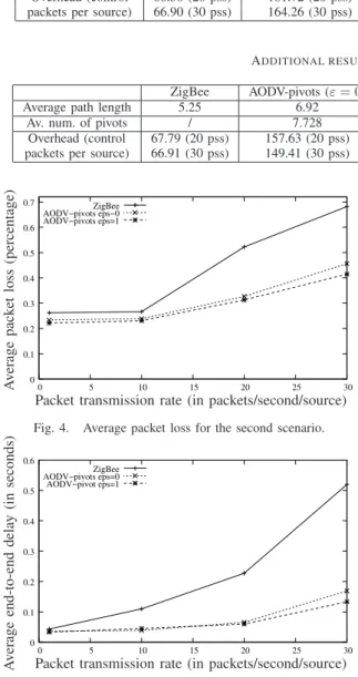
D. Results for the second scenario
In this subsection, we show the behavior of our mechanism compared to ZigBee in the second scenario (when sources are not localized in the same area).
Figures 4 and 5 show respectively the average packet loss and the average end-to-end delay, as a function of the packet transmission rate. The general behavior of the results of ZigBee and AODV-pivots is similar to the general behavior for the first scenario (see Figures 2 and 3). However, the gain of AODV-pivots is lower than the one obtained for the first scenario. Indeed, in the second scenario, as sources are dispatched far away from each other, the shortest paths from sources to the sink is not as congested as in the first scenario
TABLE I
ADDITIONAL RESULTS FOR THE FIRST SCENARIO.
ZigBee AODV-pivots (𝜀 = 0) AODV-pivot (𝜀 = 1) Math. model (𝜀 = 0) Math. model (𝜀 = 1)
Average path length 6.45 9.125 9.893 8.015 8.72
Av. num. of pivots / 17.708 15.997 14 9
Overhead (control 68.30 (20 pss) 181.72 (20 pss) 179.45 (20 pps) / / packets per source) 66.90 (30 pss) 164.26 (30 pss) 165.83 (30 pps) / /
TABLE II
ADDITIONAL RESULTS FOR THE SECOND SCENARIO.
ZigBee AODV-pivots (𝜀 = 0) AODV-pivots (𝜀 = 1) Math. model (𝜀 = 0) Math. model (𝜀 = 1)
Average path length 5.25 6.92 7.63 6.23 6.54
Av. num. of pivots / 7.728 6.54 5.5 3.5
Overhead (control 67.79 (20 pss) 157.63 (20 pss) 160.97 (20 pps) / / packets per source) 66.91 (30 pss) 149.41 (30 pss) 151.85 (30 pps) / /
ZigBee AODV−pivots eps−0 AODV−pivots eps=1 0 0.1 0.2 0.3 0.4 0.5 0.6 0.7 0 5 10 15 20 25 30
Packet transmission rate (in packets/second/source)
A v erage p ack et loss (percentage)
Fig. 4. Average packet loss for the second scenario.
ZigBee AODV−pivots eps=0 AODV−pivot eps=1 0 0.1 0.2 0.3 0.4 0.5 0.6 0 5 10 15 20 25 30
Packet transmission rate (in packets/second/source)
A v erage end-to-end delay (in seconds)
Fig. 5. Average end-to-end delay for the second scenario.
(there is still one congested path from the middle of the network to the sink, as this path is shared by two sources).
Table II reports the values of the average path length, number of pivots and number of control packets. Both the average path length and the overhead are slightly smaller than for the first scenario (see Table I). This is due to the fact that sources are closer to the sink in the second scenario. The overhead of ZigBee is not impacted significantly: the RREQs are still broadcasted in the whole network, although the RREPs travel a shorter distance.
VI. CONCLUSIONS
In this paper, we improve the AODV-based ZigBee routing protocol by the use of intermediate nodes called pivots. We
describe a set of rules to select good pivots, and we formalize these rules using a mathematical model. Through simulations, we show that our approach improves ZigBee in terms of average packet loss (which is reduced by up to 36% for 30 pss) and average end-to-end delay (which is reduced by up to 78% for 30 pss), while maintaining a number of control packets small. A mathematical model to derive the average number of pivots and the average path length is also provided. Results comparison shows the impact of not considering in the mathematical model the RREQs/RREPs mechanism to discover pivots. The model could be exploited for improving the pivots discovery procedure, with the aim of decreasing the overhead.
REFERENCES
[1] IEEE 802.15, “Part 15.4: Wireless medium access control (MAC) and physical layer (PHY) specifications for low-rate wireless personal area networks (WPANs),” ANSI/IEEE, Standard 802.15.4 R2006, 2006. [2] ZigBee Alliance, “ZigBee Specification,” ZigBee Standards
Organiza-tion, Standard Zigbee 053474r17, January 2008.
[3] J. Sun, Z. Wang, H. Wang, and X. Zhang, “Research on routing protocols based on ZigBee network,” in Intelligent Information Hiding and Multimedia Signal Processing (IIHMSP), vol. 1, 2007, pp. 639–642. [4] J. Li, X. Zhu, N. Tang, and J. Sui, “Study on ZigBee network architecture and routing algorithm,” in Signal Processing Systems (ICSPS), 2010, pp. 389–393.
[5] C. Gezer, M. Niccolini, and C. Buratti, “An ieee 802.15.4/zigbee based wireless sensor network for energy efficient buildings,” in IEEE Workshop on Advances in Wireless Sensor and Actuator Networks, WiMob, 2010.
[6] L. Casone, “Improving many-to-one traffic flowing in multi-hop 802.15.4 WSNs using a MAC-level fair scheduling,” in Mobile Ad hoc and Sensor Systems (MASS), 2007, pp. 1–7.
[7] X. Xu, D. Yuan, and J. Jian Wan, “An enhanced routing protocol for ZigBee/IEEE 802.15.4 wireless networks,” in Future Generation Communication and Networking (FGCN), vol. 1, 2008, pp. 294–298. [8] A. Bhatia and P. Kaushik, “A cluster based minimum battery cost
AODV routing using multipath route for ZigBee,” in IEEE International Conference on Networks (ICON), 2008.
[9] D. Bein, “Fault-tolerant k-fold pivot routing in wireless sensor net-works,” in 41st Hawaii International Conference on System Sciences, 2008.
[10] J. S. Lee, J. P. Ryu, and K. J. Han, “Efficient routing scheme using pivot node in wireless sensor networks,” in ICCS, ser. LNCS, no. 4490, 2007, pp. 574–577.
[11] N. El Rachkidy, A. Guitton, and M. Misson, “Pivot routing improves wireless sensor networks performance,” JNW (Journal of Networks), 2012.