Receptor modeling of C₂?C₇ hydrocarbon sources at an urban background site in Zurich, Switzerland: changes between 1993?1994 and 2005?2006

HAL Id: hal-00296534

https://hal.archives-ouvertes.fr/hal-00296534

Submitted on 5 May 2008

HAL is a multi-disciplinary open access

archive for the deposit and dissemination of

sci-entific research documents, whether they are

pub-lished or not. The documents may come from

teaching and research institutions in France or

abroad, or from public or private research centers.

L’archive ouverte pluridisciplinaire HAL, est

destinée au dépôt et à la diffusion de documents

scientifiques de niveau recherche, publiés ou non,

émanant des établissements d’enseignement et de

recherche français ou étrangers, des laboratoires

publics ou privés.

urban background site in Zurich, Switzerland: changes

between 1993?1994 and 2005?2006

V. A. Lanz, C. Hueglin, B. Buchmann, M. Hill, R. Locher, J. Staehelin, S.

Reimann

To cite this version:

V. A. Lanz, C. Hueglin, B. Buchmann, M. Hill, R. Locher, et al.. Receptor modeling of C2?C7

hydrocarbon sources at an urban background site in Zurich, Switzerland: changes between 1993?1994

and 2005?2006. Atmospheric Chemistry and Physics, European Geosciences Union, 2008, 8 (9),

pp.2313-2332. �hal-00296534�

www.atmos-chem-phys.net/8/2313/2008/ © Author(s) 2008. This work is distributed under the Creative Commons Attribution 3.0 License.

Chemistry

and Physics

Receptor modeling of C

2

–C

7

hydrocarbon sources at an urban

background site in Zurich, Switzerland: changes between

1993–1994 and 2005–2006

V. A. Lanz1, C. Hueglin1, B. Buchmann1, M. Hill1, R. Locher2, J. Staehelin3, and S. Reimann1

1_{Empa, Swiss Federal Laboratories for Materials Testing and Research, Laboratory for Air Pollution and Environmental} Technology, 8600 Duebendorf, Switzerland

2_{ZHAW, School of Engineering, Institute of Data Analysis and Process Design IDP, 8401 Winterthur, Switzerland} 3_{Institute for Atmospheric and Climate Science, ETH Zurich, 8092 Zurich, Switzerland}

Received: 28 November 2007 – Published in Atmos. Chem. Phys. Discuss.: 18 January 2008 Revised: 7 April 2008 – Accepted: 14 April 2008 – Published: 5 May 2008

Abstract. Hourly measurements of 13 volatile hydrocar-bons (C2–C7) were performed at an urban background site in Zurich (Switzerland) in the years 1993–1994 and again in 2005–2006. For the separation of the volatile organic compounds by gas-chromatography (GC), an identical chro-matographic column was used in both campaigns. Changes in hydrocarbon profiles and source strengths were recovered by positive matrix factorization (PMF). Eight and six factors could be related to hydrocarbon sources in 1993–1994 and in 2005–2006, respectively. The modeled source profiles were verified by hydrocarbon profiles reported in the literature. The source strengths were validated by independent mea-surements, such as inorganic trace gases (NOx, CO, SO2), methane (CH4), oxidized hydrocarbons (OVOCs) and mete-orological data (temperature, wind speed etc.). Our analysis suggests that the contribution of most hydrocarbon sources (i.e. road traffic, solvents use and wood burning) decreased by a factor of about two to three between the early 1990s and 2005–2006. On the other hand, hydrocarbon losses from natural gas leakage remained at relatively constant levels (−20%). The estimated emission trends are in line with the results from different receptor-based approaches reported for other European cities. Their differences to national emission inventories are discussed.

Correspondence to: V. A. Lanz (valentin.lanz@empa.ch)

1 Introduction

Air pollutants can have adverse impacts on human health, most notably on the respiratory system and circulation (Nel, 2005), acidify and eutrophicate ecosystems (Matson et al., 2002), diminish agricultural yields, corrode materials and buildings (Primerano et al., 2000), and decrease atmospheric visibility (Watson, 2002). Organic gases and particles can both be directly emitted into the atmosphere, e.g. by fos-sil fuel combustion, or secondarily formed and decomposed there by chemical reactions and/or gas-to-particle conver-sions (Fuzzi et al., 2006). Volatile organic compounds (VOCs) have several important impacts: while only some of them are toxic to humans, e.g. benzene (WHO, 1993), or relevant greenhouse gases, e.g. methane (Forster et al., 2007), all VOCs are oxidized in the atmosphere and most are thereby involved in the formation of secondary pollutants, such as ozone (O3), and secondary organic aerosol (SOA). Ambient VOC measurements became important since the 1950s (Eggertsen and Nelsen, 1958) due to summer smog phenomena, first and foremost due to high O3levels in the Los Angeles basin. The identification and quantification of VOC sources is therefore a necessary step to mitigate air pol-lution.

Receptor models were developed to attribute measured ambient air pollutants to their emission sources. Depending on the degree of prior knowledge of the sources, a chemical mass balance (CMB; composition of the emission sources is known), a multivariate receptor model (no a priori knowl-edge) or a hybrid model in between these extreme cases is most appropriate (Hopke, 1988; W˚ahlin, 2003; Christensen

Table 1. Mean concentrations and standard deviations [ppb] of the 13 considered hydrocarbon species for the years 2005–2006 (n=8912)

and values for 1993–1994 (n=7606) in brackets. Detection limits (DL, in ppt) and the relative measurement error (coefficient of variation,

CV) for each hydrocarbon species as used for PMF are also given.∗Ethane and ethyne concentrations in 1993–1994 were partially imputed.

∗∗_{Please consider the paragraph on nomenclature in Sect. 2.1.1.}

species synonym formula mean conc. [ppb] std. dev. [ppb] DL [ppt] CV [rel.]

ethane dimethyl C₂H₆ 2.34 (3.03)∗ 1.32 (2.17) 10 (15) 0.02 (0.05) ethene ethylene C2H4 1.85 (3.03) 1.38 (2.54) 10 (15) 0.02 (0.05) propane n-propane C3H8 1.25 (1.43) 0.87 (0.89) 7 (10) 0.02 (0.05) propene propylene C3H6 0.42 (0.90) 0.32 (0.76) 7 (10) 0.02 (0.05) ethyne acetylene C2H2 1.13 (3.87)∗ 0.74 (3.09) 10 (8) 0.03 (0.05) isobutane 2-methylpropane C4H10 0.59 (0.94) 0.44 (0.72) 5 (8) 0.02 (0.10) butane n-butane C4H10 0.99 (2.76) 0.78 (2.04) 5 (8) 0.03 (0.10) isopentane 2-methylbutane C₅H₁₂ 1.24 (2.96) 1.02 (2.32) 5 (7) 0.03 (0.10) pentane n-pentane C5H12 0.48 (0.94) 0.35 (0.68) 4 (7) 0.03 (0.10) isohexanes (sum) ∗∗ C₆H₁₄ 0.86 (1.17) 0.68 (0.96) 3 (7) 0.03 (0.08) hexane n-hexane C6H14 0.13 (0.29) 0.16 (0.23) 3 (6) 0.03 (0.10) benzene benzol C6H6 0.38 (0.95) 0.27 (0.68) 3 (5) 0.03 (0.05) toluene methylbenzene C7H8 1.37 (2.57) 1.15 (2.37) 3 (4) 0.03 (0.05)

et al., 2006). The first multivariate source apportionment studies were based on the elemental composition of partic-ulate matter (e.g. Blifford and Meeker, 1967). In contrast to organic species, element concentrations (e.g. of airborne metals) do not change because of degradation or secondary formation in the atmosphere. Given that their sources emit those elements in constant proportions over time, the cal-culated receptor profiles can directly be related to sources. More recently, receptor models have also been applied to or-ganic compounds since detailed chemical information about the organic gas- and aerosol-phase is available (e.g. using high-resolution gas-chromatography, Schauer et al., 1996, or aerosol mass spectrometry, Lanz et al., 2007). However, the fundamental assumption of non-reactivity or mass con-servation (Hopke, 2003) can be violated and the calculated factors may not always be directly related to emission pro-files but have to be interpreted as aged propro-files (depending on the selected species and measurement location). There-fore, a flexible model such as positive matrix factorization (PMF; Paatero and Tapper, 1994) is favorable to model VOC concentration matrices. Furthermore, PMF modeling allows for any changes (e.g. local differences) in the nature of the VOC sources. The PMF2 program (Paatero, 1997) uses a sta-ble algorithm to estimate source strengths and profiles from multivariate data sets (bilinear receptor-model). Miller et al. (2002) concluded for simulated data that PMF was su-perior in recovering VOC sources compared to other recep-tor models based on standard CMB (Winchester and Nifong, 1971), principal component analysis (Blifford and Meeker, 1967) or UNMIX, a multivariate receptor model developed by Henry (2003). Also Jorquera and Rappengl¨uck (2004) found PMF resolved VOC profiles more reliable than profiles resolved by UNMIX, while Anderson et al. (2002) found the

results of the two models to be in good agreement. Fur-ther evidence that bilinear unmixing by PMF2 can be used to model VOC data was provided for the Texas area (Buzcu and Frazier, 2006), where for certain emission situations (e.g. wind directional dependencies of point sources etc.) an enhanced PMF was favorable (Zhao et al., 2004).

Due to the environmental problems mentioned above, ab-atement strategies have been developed and implemented for the reduction of VOC emissions. In fact, the sum of non-methane VOCs at the urban background location in Zurich (Switzerland), as studied in this article, decreased by -50% between 1986 and 1993 and again by -30% from the early 1990s to today (Fig. 1). For 1993–1994, about 20 volatile hydrocarbon species were determined at Zurich-Kaserne by hourly resolved gas-chromatography (GC-FID). For 2005– 2006, more than 20 hydrocarbons were measured again at the same site (13 of them were measured during both peri-ods and are summarized in Table 1 and Fig. 2). The same chromatographic column was used for both campaigns. By PMF modeling of hydrocarbon observations in 1993–1994 and in 2005–2006 we describe the underlying factors of each data set. The factors recovered by multivariate PMF mod-eling are related to hydrocarbon source profiles and source strengths. This attribution needs to be verified by means of collocated measurements (inorganic trace gases, oxidized hydrocarbons, meteorology), by time series analysis of the source strengths as well as by published VOC profiles and emission factors from the literature. The decrease in ambi-ent VOC concambi-entrations between the early 1990s and today (2005–2006) is explained by comparing the factor analytical results for both data sets. The contribution of different emis-sion sources to this trend is discussed.

0.40 0.35 0.30 0.25 0.20 0.15 0.10 ppmC 2005 2000 1995 1990 t-NMVOC, Zürich-Kaserne (1986-2006) 2005-06 1993-94

Fig. 1. Total concentrations [ppmC] of non-methane volatile

or-ganic compounds (t-NMVOC) at an urban background site (Zurich, Switzerland) measured by a standard FID (flame ionization detec-tor). Speciated VOC data is available for 1993–1994 and since 2005 (red and blue points).

2 Methods

2.1 Measurements

2.1.1 Hydrocarbon measurements

The measurements at Zurich-Kaserne (410 m a.s.l.) are rep-resentative for an urban background site in Zurich, Switzer-land. The sampling site is located in a public backyard near the city center. The earlier VOC measurements in 1993–1994 were presented by Staehelin et al. (2001). The time spans in this study included 4 June 1993 to 6 October 1994 and 4 June 2005 to 6 October 2006.

18 hydrocarbons were measured quasi-continuously in Zurich between 1993 and 1994: first, ambient air was passed through a Nafion Dryer to minimize its water con-tent and then hydrocarbons were trapped on an adsorption-desorption unit (VOC Air Analyzer, Chrompack) by using a multi-stage adsorption tube held at −25◦C. The flow of air through the trap was at 10 ml min−1 and the trapping time was 30 min, yielding a total volume of 300 ml of sam-pled air. Then the trap was heated to 250◦C for transfer-ring the VOCs to a cryo-focussing trap (PoraPLOT Q), held at −100◦C. Finally, concentrated VOCs were passed onto the analytical PLOT column (Al2O3/KCl, 50 m×0.53 mm, Chrompack) by heating to 125◦C. The analysis was per-formed by gas chromatography-flame ionization detection (GC-FID, Chrompack). Calibration was performed regularly by diluting a commercial standard with zero air to the lower ppb (parts per billion by volume) range.

22 hydrocarbons were measured quasi-continuously in 2005–2006: First, ambient air was passed through a Nafion Dryer to minimize its water content and was then ex-tracted from hydrocarbons using an adsorption-desorption unit (Perkin-Elmer, TD), equipped with a multi-stage

micro-5 4 3 2 1 0 ethane* ethene

propane propene ethyne*

isobutane butane isopentane pentane S-isohexanes hexane benzene toluene 1993-1994 2005-2006 ppb

Fig. 2. Averaged values for the 13 hydrocarbons measured in 1993–

1994 (red) and in 2005–2006 (blue) at Zurich-Kaserne. *Ethane and ethyne measurements in 1993–1994 were partially imputed (see text, Sect. 2.2.3). A definition of “S-isohexanes” is given in Sect. 2.1.1.

trap held at −30◦C by means of a Peltier element. The flow of air through the trap was 20 ml min−1and the trapping time was 15 min, yielding a total volume of 300 ml of sampled air. After flushing with helium to reduce the water vapor content the trap was rapidly heated to 260◦C for desorption of the hydrocarbons onto the analytical PLOT column (Al2O3/KCl, 50 m×0.53 mm, Varian). The analysis was performed by gas chromatography-flame ionization detection (GC-FID, Agi-lent 6890). Calibrations were performed regularly using a standard which contains the analyzed hydrocarbons in the lower ppb range (National Physical Laboratory, UK).

13 hydrocarbon species were measured in both data sets (summarized in Table 1 and Fig. 2) and used for the statisti-cal analysis. The chromatographic column for separation of the VOCs is identical for the two measurement periods. This is an advantage for the comparison of the two data sets, al-though newest developments use two-dimensional gas chro-matography (GC×GC) to separate overlapping peaks (e.g. Bartenbach et al., 2007). Trapping efficiency was below 100% for the C2hydrocarbons, which however was corrected by a specific calibration factor.

The hydrocarbon species in this article are named based on IUPAC. As an exception, the term “sum of isohexanes” (S-isohexanes) is used, which refers to the added concentrations of 2-methylpentane and 3-methylpentane (1993–1994), but for 2005–2006 the sum includes 2,2-dimethylbutane and 2,3-dimethylbutane as well.

2.1.2 Ancillary data

In addition to the hydrocarbons, about 20 different, hourly resolved OVOCs are available at Zurich-Kaserne for

campaigns in summer 2005 and winter 2005/2006. The measurements were performed by GC-MS (gas chromato-graph with mass spectrometer) and summarized in Legreid et al. (2007a). Inorganic trace gases (NOx, CO, SO2), meteoro-logical parameters (temperature, wind speed etc.), methane (CH4), and total non-methane VOCs (t-NMVOC) were mea-sured by standard methods (Empa, 2006). Measurements of t-NMVOCs are performed continuously by a flame ioniza-tion detector (FID) (APHA 360, Horiba). For separaioniza-tion be-tween CH4and t-NMVOCs the air sample is divided into two parts. One part is directly introduced into the FID, while the second part is lead through a catalytic converter to remove the NMVOCs. The outcome of both lines is measured al-ternately and the t-NMVOC concentration is calculated from the difference of the two measurements.

2.2 Data analysis and preparation 2.2.1 Unmixing multivariate observations

Linear mixing of observable quantities is the basis to all re-ceptor models and can be represented by the following equa-tion (Henry, 1984):

xi=giF+ei, (1)

where xi represents the i-th multivariate observation

(vec-tor of m variables) and is approximated by linear combi-nations of the loadings or source profiles, F, and scores or source strengths, gi, up to an error vector, ei. Chemical

mass balance models were designed for estimation of source strengths, gi (a p-dimensional vector), for given numerical

values of F, representing a p×m-matrix of the source pro-files, and a specified number of assumed factors or sources p. Bilinear receptor models, on the other hand, are most useful when very little or no prior knowledge about the sources is assumed. In such a case, both gi and F have to be estimated,

and p has to be determined by exploratory means. Paatero and Tapper (1994) have proposed to solve Eq. (1) by a least-square algorithm minimizing the uncertainty weighted error (“scaled residuals”): eij/sij=(xij− ˆyij)/sij, ˆyij= p X k=1 gikfkj, (2)

The associated software PMF2 (Paatero, 1997) minimizes the sum of (eij/sij)2(called Q) for all samples i=1. . .n and

all variables j =1. . .m. In practice, an enhanced Q is to be minimized, accounting e.g. for penalty terms that ensure a non-negative solution to Eq. (1). This approach implicitly assumes that uncertainties, sij, for each element of the

multi-variate data set, xij, are known. For VOC species, an ad hoc

measurement uncertainty, s′_ij, has been suggested by Anttila et al. (1995) and was used in many studies (e.g. Fujita et al., 2003, and Hell´en et al., 2006):

s′_ij=q4(DL)2_j+((CV )jxij)2, (3)

where DL represents the detection limit (as an absolute con-centration value) and the coefficient of variation, CV, ac-counts for the relative measurement error determined by cal-ibration of the instruments. The DLs equal five times the baseline noise of the species’ chromatograms, whereas the CVs are the relative standard deviations of six repeated mea-surements of a real-air standard in the range of ambient con-centrations. Following this method, both DL and CV are species-specific and given in Table 1 for the present hydro-carbon data sets. The total uncertainties, sij, in Eq. (2)

cal-culate as

sij=s

′

ij+d(maxhxij, ˆyiji), (4)

where parameter d symbolizes the relative modeling uncer-tainty and ˆyij the model for xij.

2.2.2 Model specifications and reactivity

For the presented results, the PMF2 program was run with default settings (robust mode, central rotation induced by fpeak=0.0, outlier thresholds for the scaled residuals of −4 and 4), but the error model (EM=−14) was adjusted for am-bient data. Two-dimensional scatter plots of factor contribu-tions showed edges parallel to the coordinate axes, which is indicating that the chosen rotation has low ambiguity (heuris-tic approach by Paatero et al., 2005). A modeling uncer-tainty d>0% is needed as two basic assumptions about PMF are likely to be violated in this study (constant source pro-files over time and non-reactivity of the species). The results shown here were calculated by setting d=10%, which rep-resents an arbitrary but non-critical choice as will be shown below. We further assumed that the VOC variability at the ur-ban site Zurich-Kaserne is generally driven by source activi-ties rather than by ageing of the compounds (see Sects. 3.3.2 and 3.3.3); VOC transport time from source to receptor was assumed to be less than 0.5 day on average, which is smaller than the lifetime of propene, the most reactive compound an-alyzed in the study.

2.2.3 Missing values

In 1993–1994, missing ethane and ethyne concentrations had to be imputed for n=3450 and n=1500 samples, respec-tively (∼5% of data matrix). These values were missing due to data acquisition problems. Row-wise deletion of those missing values (i.e. a sample is excluded when at least one species is not available) would have caused a loss of 50% of the data. We instead have used the k-nearest neighbor (knn) method to estimate those missing values (function knn of the EMV package in R, The R Foundation for Statisti-cal Computing; www.r-project.org). Additional VOCs were considered for the nearest-neighbor calculations (e.g. 2,2,4-trimethylpentane, 2-methylpropene, and heptane). Advan-tages of data imputation by multivariate nearest neighbor methods in the field of atmospheric research were evaluated

by Junninen et al. (2004): they are particularly important for practical applications as they are fast, perform well, and do not generate new values in the data. We calculated (by repet-itively and randomly assigning missing values to known val-ues) that the relative uncertainty of this imputational method is about 48% (1 σ ) for ethane and about 32% (1 σ ) for ethyne. Calculating the uncertainty matrix, the imputed concentra-tion values of ethane and ethyne were multiplied by 0.96 (2 σ ) and 0.64 (2 σ ), respectively, and the square of this prod-uct was added to the error as stated by Eq. (3):

s′_ij=q4(DL)2_j+(CV )2

jxij2+(2σ xij)2, xijimputed (5)

In summary, this additional term down-weights the imputed values by a factor of about 10. Even though the imputed values have a minor weight in the minimization algorithm of PMF2, factors characterized by ethane or ethyne for the 1993–1994 data should nevertheless be carefully interpreted. 2.2.4 Outliers in the data (contamination-type)

Propane peaks up to 400 ppb (2005–2006) and 200 ppb (1993–1994) could be observed and were most probably caused by local barbecue events. We have defined extreme observations to be larger than µ+σ (2005–2006) and µ+2 σ (1993–1994): About 70 samples were identified and ex-cluded from both data sets in order to not distort the factor analysis. A detailed inspection of the deleted samples re-vealed that these propane peaks mostly occurred on/before weekends and holidays during the summery season, support-ing the hypothesis of local barbecue emissions in the public backyard surrounding the measurement site. In 2005–2006, a threshold of σ rather than 2 σ was needed to identify a sim-ilar fraction (∼1%) of outliers. These contamination-type propane outliers were excluded prior to PMF analysis.

3 Results and discussion

3.1 Determination of the number of factors (p)

The determination of the number of factors p is a critical step for receptor-based source apportionment methods, es-pecially for bilinear models, where very little prior knowl-edge about the sources is assumed. Mathematically perfect matrix decompositions into scores and loadings do not guar-antee that the solutions are physically meaningful and can be interpreted. Here, we followed the philosophy that an appro-priate number of factors has to be determined by means of interpretability and physical meaningfulness as already pro-posed earlier (e.g. by Li et al., 2004; Buset et al., 2006; Lanz et al., 2007, 2008). Mathematical diagnostics are however indispensable to corroborate the chosen solution and to de-scribe the mathematical aspect of its explanatory power.

For the recently (2005–2006) measured VOCs, p=6 fac-tors can be interpreted and are discussed in Sects. 3.4 and 3.5.

Choosing less factors, p<6, coerces two profiles (attributed to “solvent use” and “gasoline evaporation”; see Sect. 3.4). On the other hand, by choosing more factors, p>6, a fac-tor splits from the “gasoline evaporation” facfac-tor (the sum of two split contributions is very similar, R=0.97, to the gaso-line source contributions retrieved with p=6). We therefore consider the 6-factor PMF solution for further analyses of the VOC sources in 2005–2006. For the earlier VOC series (1993–1994), we have most confidence in the 8-factor PMF solution: when assuming 8 factors, for each of the 6 factors found in 2005–2006 a similar factor is found as in the ear-lier measurements (plus a toluene source and an additional, combustion-related source). This can not be observed for so-lutions where more than 8 factors or less than 8 factors were imposed.

The data sets from 1993–1994 and 2005–2006 had to be described by a different number of factors each (eight and six, respectively) in order to account for the different emission situations: two factors were absent in the 2005– 2006 data, which can be explained by policy regulations (see Sects. 3.5 and 4).

3.2 Mathematical diagnostics

More than 93% and 96% of the variability of the VOC species could be explained on average by the 6-factor PMF model (2005–2006) and the 8-factor PMF model (1993– 1994), respectively (see concept of explained variation; Paatero, 2007). Using the proposed model we can further explain on average 97% and 99% of the total concentration of the 13 hydrocarbons (in ppb) measured in 2005–2006 and 1993–1994, respectively. These latter ratios represent an av-erage modeled to measured hydrocarbon concentration: ratio = (1/n) n X i=1 ( p X k=1 gik/ m X j =1 xij), (6)

where xij are the observed concentration values, gik

repre-sents concentrations modeled by k=1...p factors (note that the factor profiles were normalized to unity,Pm

j =1fkj=1), and n is the number of samples consisting of m species. This measure is only meaningful, if Pp

k=1gik−

Pm

j =1xij≤0 is

approximately fulfilled for virtually all samples and if there is little scatter in the data, which is the case here. We addi-tionally calculated the R2 of the linear regression, lm, data versus modeled values

lm( m X j =1 xij ∼ p X k=1 gik), (7)

yielding R2=0.99 in both cases (2005–2006 and 1993–1994, respectively). Thus, almost all variance in the total concen-tration of the 13 hydrocarbons can be explained by the PMF based model.

For both models, less than 1% of all data points (about 100 000 for both data sets) exceeded the model outlier

thresholds for the scaled residuals, |eij/sij|>4, and were

down-weighted (Sect. 2.2). The Q-value, the total sum of scaled residuals, equals 11 275 in the robust-mode for the 1993–1994 data (n=7606, p=8). For 2005–2006 (n=8912, p=6), this value is 70 018. Thus, for both data sets the calcu-lated Q is in the order of the expected Q, estimated by mn-p(m+n) as a rule of thumb: The value of Q should approx-imately equal the degrees of freedoms (e.g. Li et al., 2004), which can be estimated by the number of independent ob-servations, mn, minus the number of estimated parameters, p(m+n). The scaled residuals for each species and both data sets are approximately normally distributed N(0, σj).

3.3 Robustness of the PMF-solutions 3.3.1 Hydrocarbon species

In order to test the robustness of the presented results, we made additional PMF runs with 21 hydrocarbons available since 2005 (the sum of butenes was deleted column-wise from the data matrix due to its abundant missing values). Isoprene and 1,3-butadiene were found to determine two ad-ditional factors almost alone due to their distinct temporal behavior in ambient air: both VOCs are rapidly removed by radical reactions. Their atmospheric lifetime is in the order of minutes to hours and these compounds therefore change the variability structure of the data matrix. However, isoprene and 1,3-butadiene accounted for less than 1% of the total con-centration (in ppb) given by the 22 hydrocarbons retrieved since 2005 at Zurich-Kaserne. Therefore, the exclusion of these latter compounds does not influence the representative-ness, but leads to more robust results. On the other side, aromatic C8hydrocarbons (m/p-xylene, o-xylene, and ethyl-benzene), which were highly correlated (R>0.97), summed up to considerable concentrations, but did not alter the vari-ability pattern in the data (see Sect. 3.5.1).

3.3.2 Reactivity and modeling uncertainty

Following the idea of Latella et al. (2005), photochemically reactive compounds j can be down-weighted depending on [Ox]l, the oxidant level (i.e. number concentrations of OH, O3, Cl and NO3 radicals), individual rate constants, kj,l

[cm3molec−1s−1], and photochemical age, t [s], resulting in a vector rj

rj = e−t P

l([Ox]lkj,l)_{, (8)}

which incorporates in the total uncertainty estimates (see Eq. 4) as follows sij=s ′ ijr −1 j +d(maxhxij, ˆyiji). (9)

Note that for measurements close to sources (t is small) or inert species (kj,l is small), this vector is rj≈1 and Eq. (9)

simplifies to the uncertainty model postulated earlier (Eq. 4;

e.g. Lee et al., 1999). The correction factors for the hydr-carbon reactivity (Eq. 8; sticking to the idea of Latella et al., 2005) were calculated assuming an average transport time from source to receptor of t=4 h and a typical OH radical concentration of 0.8×106molec cm−3(Seinfeld and Pandis, 1998). The rate constants were derived from Atkinson and Arey (2003). The correction factors in rj in the case of the

Zurich-Kaserne site lie between 0.89 and 1.00 (except for propene, where a factor of 0.66 has been calculated). Di-viding the analytical uncertainty (Eq. 3) by these correction factors and allowing a modeling uncertainty of 10% yields changes in the relative mean SCEs (source contribution esti-mates) that are smaller than 1% for each factor in 2005–2006 and less than 4% for the factors in 1993–1994. In fact, in the earlier Zurich data the strongest trend (+3.98%) in the relative mean SCEs can be observed for the “fuel combus-tion” source (factor 6), as its loading of propene (clearly the most reactive compound in our study) was almost as high as ethene (the highest peak in factor 6). This is different for the 2005–2006 data, where the propene loading in factor 6 ac-counted only half of the ethene intensity. Finally, it should be pointed out that the calculated profiles for the receptor site Zurich-Kaserne could be directly related to measured source profiles from the literature (Sect. 3.4). Thus, the assump-tion that the typical transport time from source to receptor is smaller than the atmospheric lifetime of the most reactive species (Sect. 2.2.2) seems to be justified. As shown for or-ganic aerosols (Lanz et al., 2007), it can actually be mean-ingful to interpret PMF factors as secondary and differently aged profiles. The same could hold true for more volatile organics (VOCs) as well, but was not necessary here as we measured close to the VOC emission sources (and the chosen substances are not formed secondarily in the atmosphere).

Generally, the PMF solutions of the presented data were found to be stable with respect to different uncertainty spec-ifications. In particular, the SCEs are rather insensitive to different modeling uncertainties, d. This can be shown by increasing d from 5% up to 35%, while rj is kept fixed at

unity: For the recent Zurich data (2005–2006), the largest change due to increasing the modeling uncertainty from 5% to 35% is observed for the relative mean SCEs of factor 2, namely −2.6%. For the earlier data, the SCEs are not very sensitive to modeling uncertainties neither: in analogy to the case described above, the largest change can be observed for factor 4 (1993–1994), namely +5.6%. Note that factor 4 is dominated by ethane (and ethyne), both of which were par-tially imputed. It is plausible that imputed species are more sensitive to increases of d, as the case discrimination in un-certainty levels for missing (Eq. 5) and available data points (Eq. 3) relative to their total uncertainty estimates is down-weighted.

0.25 0.20 0.15 0.10 0.05 0.00 0.30 0.20 0.10 0.00 0.4 0.3 0.2 0.1 0.0 0.6 0.4 0.2 0.0 0.30 0.20 0.10 0.30 0.20 0.10 0.00 ethane ethene

propane propene ethyne

isobutane n-butane isopentane n-pentane

S-isohexanes

n-hexane benzene toluene

factor 1 ("gasoline evaporation")

factor 2 ("solvents")

factor 3 ("propane")

factor 4 ("ethane")

factor 5 ("wood burning")

factor 6 ("fuel combustion")

PMF factors (2005-06)

Fig. 3. The profiles of the 6-factor PMF solution calculated for the

recently measured hydrocarbon data (2005–2006). Each profile’s loadings were normalized to a sum of unity. Here, S-isohexanes comprises 2-methylpentane, 3-methylpentane, 2,2-dimethylbutane, and 2,3-dimethylbutane.

3.3.3 Down-mixing of aged air masses

An aged profile was determined by averaging gas-phase mea-surements at a rural site (Rigi-Seebodenalp, 1031 m a.s.l., 40 km Southeast of Zurich) during a week-long high-pressure episode in 2005. This profile was fixed and im-posed on the factor analytical solution for the urban data from Zurich-Kaserne (410 m a.s.l.) spanning the same time inter-val.

While the aged profile was frozen during the iterative (hy-brid) model fit, n=1, 2, . . . factors were allowed to evolve freely within a non-negative subspace. The computations were carried out using the multilinear engine program, ME-2, designed by Paatero (1999). We have lately described the technical details of such an approach (Lanz et al., 2008). The resulting scores of the imposed profile (enriched with sta-ble and secondary species) did however not show the typical, strong increase during early morning hours as expected for chemically stable and secondary pollutants. Such increases

0.6 0.4 0.2 0.0 0.6 0.5 0.4 0.3 0.2 0.1 0.0 0.20 0.15 0.10 0.05 0.00 0.6 0.4 0.2 0.0 0.4 0.3 0.2 0.1 0.0 0.30 0.20 0.10 0.00 ethane ethene

propane propene ethyne isobutane n-butane isopentane n-pentane S-isohexanes n-hexane benzene toluene 0.4 0.3 0.2 0.1 0.0 0.25 0.20 0.15 0.10 0.05 0.00 factor 4 ("ethane") factor 3 ("propane")

factor 6 ("fuel combustion") factor 5 ("wood burning")

factor 1 ("gasoline evaporation")

factor 7 ("earlier traffic source") factor 2a ("non-toluene solvents")

factor 2b ("toluene")

PMF factors (1993-94)

Fig. 4. The profiles of the 8-factor PMF solution calculated for the

earlier hydrocarbon data (1993–1994). Each profile’s loadings were normalized to a sum of unity. Here, S-isohexanes equals the sum of 2-methylpentane and 3-methylpentane.

were ascribed to vertical down-mixing of air from the noctur-nal residual layer to the surface air of the planetary boundary layer (e.g. McKendry et al., 1997). We therefore concluded that highly aged and processed air masses do not signifi-cantly influence the variability in the VOC profiles studied at Zurich-Kaserne.

3.4 Hydrocarbon profiles

In this section, the factor profiles as retrieved by PMF for 1993–1994 and 2005–2006 are summarized (Table 2) and discussed. We introduce a tentative attribution of PMF fac-tors to emission sources based on a priori knowledge such as published source profiles. The factors underlying the re-cent measurements (Fig. 3) and the ones explaining the ear-lier VOC data (Fig. 4) are compared with each other, with reference profiles found in the literature, and with profiles reported in Staehelin et al. (2001).

The factors for the recent data (2005–2006) were sorted on the basis of explained variance (Paatero, 2007). The factors

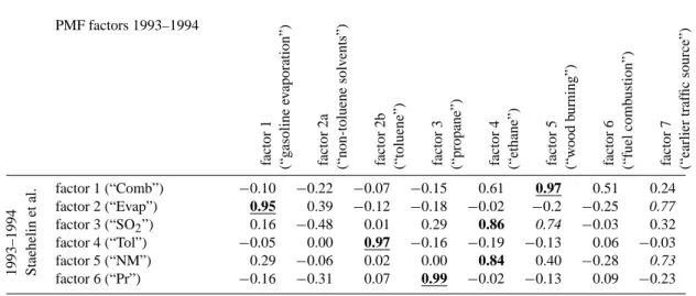
Table 2. Comparison of the 8-factor PMF (1993–1994 data) with the 6-factor PMF solution for 2005–2006. A total of 13

hydrocar-bons (n=13) were considered for the PMF analysis. The comparison is based on the correlation coefficient: 0.7≤R<0.8, 0.8≤R<0.9, and 0.9≤R≤1.0. PMF factors 1993–1994 factor 1 (“g asoline ev aporation”) factor 2a (“non-toluene solv ents”) factor 2b (“toluene”) factor 3 (“propane”) factor 4 (“ethane”) factor 5 (“w ood b urning”) factor 6 (“fuel comb ustion”) factor 7 (“earlier traf fic source”)

factor 1 (“gasoline evaporation”) 0.92 0.38 −0.14 −0.20 −0.16 −0.20 −0.31 0.71

factor 2 (“solvents”) 0.42 0.78 −0.20 −0.14 −0.22 −0.21 −0.20 0.34

2005–2006 PMF

factors factor 3 (“propane”)_{factor 4 (“ethane”) −0.15}0.13 −0.40_{−0.27 −0.06}−0.14 0.94_0.10 0.03_{0.94 −0.05}−0.08 −0.08_0.17 −0.16_−0.17

factor 5 (“wood burning”) −0.28 −0.19 −0.13 −0.09 0.22 0.97 0.43 0.10

factor 6 (“fuel combustion”) −0.24 −0.28 0.12 −0.09 −0.25 0.42 0.90 −0.36

calculated for the earlier data (1993–1994) were rearranged according to the order of the factors retrieved from the recent data (2005–2006).

3.4.1 Profiles for the years 2005–2006

The variability described by factor 1 is dominated by con-tributions of (iso-)pentane, S-isohexanes, (iso-)butane and it includes toluene and benzene (Fig. 3). This feature is shared by gasoline evaporation as well as gasoline combus-tion as can be deduced from the VOC profiles reported in Theloke and Friedrich (2007). In fact, the first PMF com-puted factor correlates well with the following reference pro-files found therein: two-stroke engine, urban mode, warm phase (R=0.94, n=13, n: number of individual hydrocarbons) and cold start phase (R=0.94, n=13) as well as with gasoline evaporation (R=0.97, n=7). Thus, based on its fingerprint alone factor 1 could be related to gasoline combustion and/or gasoline evaporation. A more specific interpretation of this first factor is given in Sect. 3.5.1.

In factor 2, prominent toluene, S-isohexanes and isopen-tane contributions can be observed and most of the toluene (61%), S-isohexanes (52%), hexane (48%), pentane (40%) and isopentane (40%) variability is explained by the second factor. This factor is only weakly influenced by the variabil-ity of combustion related C2–C4hydrocarbons (<10%). We therefore attribute this factor to solvent use.

Given the hydrocarbon fingerprint only, factor 3 (propane and butane) and factor 4 (ethane) could be related to many different sources (natural gas distribution and/or combustion, gas grill emissions, petrol gas vehicles, propellants etc.). Be-cause benzene and toluene do not influence this third fac-tor, we tend to attribute these factors to gas leakage or a

“clean” combustion source. Furthermore, factor 4 is domi-nated by ethane and potentially could also represent an aged background profile; ethane is the longest lived species con-sidered in this study. In the Northern Hemisphere, ethane and propane are principally related to natural gas exploita-tion (Borbon et al., 2004), but the presence of background ethane needs to be considered as well. Additional analyses of the source strengths are necessary for further interpreta-tions (Sect. 3.5.3).

The hydrocarbon profile of factor 5 is similar to a wood burning profile from a flaming stove fire, which is character-ized by ethene and ethyne as can be derived from Barrefors and Petersson (1995) (Fig. 5). Further, factor 5 is also corre-lated (R=0.75, n=9) with the one reference profile for wood combustion provided in Theloke and Friedrich (2007). Ac-cording to both studies, more benzene than toluene is emit-ted by wood fires ranging from 3:1 ppb/ppb to 8:1 ppb/ppb. This latter value is close to a ratio of 6:1 ppb/ppb in factor 5 (2005–2006). Further, the sum of isohexanes is enhanced in factor 5, which is possibly due to furan derivates. Furan is re-leased by wood smoke (Olsson, 2006). Note that the isohex-anes measured in 1993–1994 only included 2-methylpentane and 3-methylpentane, which are not likely to interfere with furan derivates. This would explain the absence of the sum of isohexanes in the wood burning profile computed for the ancient data (Fig. 4). All these findings suggest that factor 5 can be related to wood burning.

Factor 6 is closest (R=0.82, n=13) to the profile mea-sured for diesel vehicles in the urban mode and warm phase within the database compiled by Theloke and Friedrich (2007; source profiles representing 87 different anthro-pogenic emission categories in Europe). As observed for

Table 3. Comparison of the 8-factor PMF (1993–1994 data) with factors reported in literature (Staehelin et al., 2001). A total of 12

hydrocarbons (n=12) were considered in both studies. The comparison is based on the correlation coefficient: 0.7≤R<0.8, 0.8≤R<0.9, and 0.9≤R≤1.0. PMF factors 1993–1994 factor 1 (“g asoline ev aporation”) factor 2a (“non-toluene solv ents”) factor 2b (“toluene”) factor 3 (“propane”) factor 4 (“ethane”) factor 5 (“w ood b urning”) factor 6 (“fuel comb ustion”) factor 7 (“earlier traf fic source”) factor 1 (“Comb”) −0.10 −0.22 −0.07 −0.15 0.61 0.97 0.51 0.24 factor 2 (“Evap”) 0.95 0.39 −0.12 −0.18 −0.02 −0.2 −0.25 0.77 1993–1994 Staehelin et al. factor 3 (“SO2”) 0.16 −0.48 0.01 0.29 0.86 0.74 −0.03 0.32 factor 4 (“Tol”) −0.05 0.00 0.97 −0.16 −0.19 −0.13 0.06 −0.03 factor 5 (“NM”) 0.29 −0.06 0.02 0.00 0.84 0.40 −0.28 0.73 factor 6 (“Pr”) −0.16 −0.31 0.07 0.99 −0.02 −0.13 0.09 −0.23

wood fires, gasoline and diesel powered vehicles typically release more alkenes than alkanes as well, but the latter sources emit more toluene than benzene (Staehelin et al., 1998). Increasing toluene-to-benzene ratios during the last decade can be derived from emission factors as calculated from a nearby tunnel study: while this ratio was 16:10 [mg km−1/mg km−1] in 1993 (Staehelin et al., 1998), a ra-tio of 5:2 [mg km−1/mg km−1] was reported for the year 2004 (Legreid et al., 2007a). Let both species be emitted into an air volume of unity at a distance of unity: we then can also say that the ratio toluene:benzene increased from about 1:1 ppb/ppb to 2:1 ppb/ppb from the early 1990s un-til today. This change is perfectly represented by factor 6 (comp. 1993–1994 vs. 2005–2006) and has been caused by restriction of benzene content in car fuel. The large ratio isopentane-to-pentane as found in factor 6 (namely 10:1) is shared with diesel reference profiles, where a ratio up to 7:1 can be calculated (Theloke and Friedrich, 2007). All in all, we interpret factor 6 as fuel combustion with significant con-tributions from diesel vehicles.

3.4.2 Profiles for the years 1993–1994

In this section, the PMF retrieved hydrocarbon profiles from the 1993–1994 data are compared first with the factors for the recently measured data (2005–2006). Then, our PMF solution for the earlier data is compared to the factors analyt-ical results of a precedent study carried out by Staehelin et al. (2001).

Comparison with recent data (2005–2006)

Five very similar factors (R>0.90, n=13) as found for 2005– 2006 (Sect. 3.4.1) can be recovered from the 1993–1994 data (both data sets analyzed by bilinear PMF2). Based on the correlation coefficient, R, factors 2a, 2b, and 7 seem to be missing in the recent data (2005–2006) and the most dra-matic change can be observed for the organic solvents that were separated in the earlier data (1993–1994; represented by factor 2a and factor 2b) (Table 2 and Fig. 4).

In 1993, toluene showed a different temporal variability than the other potential organic solvents (isopentane, pen-tane, S-isohexanes, and hexane) and emerges as a distinct factor. Both factor 2a and 2b virtually only explain the vari-ability of potential solvents (Fig. 6). The distinct temporal behavior of toluene (with increased concentrations at night) is probably due to the local printing industry that was ac-tive in the 1990s but was not continued after or uses other solvents. Also Staehelin et al. (2001) identified a distinct toluene source (see Sect. 3.5). It is possible that asphalt works are represented by factor 2b as well. The addition of factor 2a and 2b (1993–1994) however yields a factor with similar loading proportions of toluene, S-isohexanes and isopentanes as found for solvents in the recent data (2005– 2006).

In terms of R, factor 7 is closest to two stroke-engines (R=0.74, n=13) within the reference data base provided by Theloke and Friedrich (2007). However, relatively promi-nent ethyne and S-isohexanes contributions (compared with other types of engines found in Theloke and Friedrich, 2007) point to gasoline driven vehicles without catalytic convert-ers, which still accounted for about 30% of the Swiss fleet in 1993–1994 (Staehelin et al., 1998).

Table 4. Correlation of measured trace gases (NOx, CO, CH4, and SO2) and total non-methane VOC, (t-NMVOC), with the PMF calculated factors for 2005–2006 (n∼8900 samples) and 1994–1995 (n∼7600 samples). 0.7≤R<0.8, 0.8≤R<0.9, and 0.9≤R≤1.0.

NOx CO SO2 CH4 t-NMVOC

PMF factors 2005–2006

factor 1 (“gasoline evaporation”) 0.64 0.63 0.24 0.39 0.72

factor 2 (“solvents”) 0.69 0.64 0.22 0.47 0.80

factor 3 (“propane”) 0.75 0.77 0.67 0.67 0.65

factor 4 (“ethane”) 0.29 0.42 0.54 0.46 0.21

factor 5 (“wood burning”) 0.66 0.80 0.58 0.64 0.56 factor 6 (“fuel combustion”) 0.76 0.84 0.59 0.53 0.71 PMF factors 1993–1994

factor 1 (“gasoline evaporation”) 0.55 0.58 0.32 0.32 0.65 factor 2a (“non-toluene solvents”) 0.71 0.76 0.45 0.45 0.77

factor 2b (“toluene”) 0.67 0.64 0.44 0.43 0.73

factor 3 (“propane”) 0.59 0.54 0.60 0.64 0.45

factor 4 (“ethane”) 0.64 0.64 0.72 0.60 0.42

factor 5 (“wood burning”) 0.87 0.89 0.75 0.64 0.71

factor 6 (“fuel combustion”) 0.88 0.91 0.64 0.58 0.83

factor 7 (“earlier traffic source”) 0.61 0.66 0.28 0.31 0.76

Comparison to Staehelin et al. (2001)

Staehelin et al. (2001) also analyzed the Zurich-Kaserne 1993–1994 data by non-negatively constraint matrix factor-ization. All six factors mentioned therein correlate well (R>0.80, n=12) with the PMF computed profiles for the 1993–1994 data (Table 3). Sources dominated by single VOC species (toluene and propane source) are here also rep-resented by one single PMF factor. The relation of the other factors is however more ambiguous, but for the reasons dis-cussed below it can not be expected that the results of the two studies are in perfect agreement:

Unlike PMF2, the algorithm used in the precedent study was based on alternating regression. Similar to the consid-erations by Henry (2003), it was also assumed by Staehe-lin et al. (2001) that the VOC sources can be identified by the geometrical implications of the receptor model Eq. (1), i.e. there are samples in the data matrix that represent single-source emissions, defining the vertices of the solution space projected onto a plane (and thereby providing starting points for the unmixing algorithm). Contrary to this proceeding, the PMF2 algorithm is started from random initial values by de-fault. In contrast to the present study, Staehelin et al. (2001) included inorganic gases and t-NMVOC in the data matrix. By expanding the data matrix its variability structure was al-tered and factors dominated by inorganic SO2 and NOx as well as t-NMVOC were identified. Different sources may have been coerced as e.g. SO2is emitted by several source types (wood burning, diesel fuel combustion etc.), and as ac-tivities of non-SO2emitting sources can be correlated with the SO2time series by coincidence or due to strong meteo-rological influence. Instead, we suggest using the inorganic

gases and sum parameters (t-NMVOC) as independent trac-ers to validate our factor interpretation. Furthermore, wood burning was not considered as potentially important emission source by Staehelin et al. (2001).

3.5 Source activities

In this section, the hydrocarbon factors are attributed to emis-sion sources based on comparisons with other, indicative compounds and meteorological data measured at the same site. Before the factors are discussed individually, we will first give a brief overview of the correlation of computed source activities with independently measured trace gases at the same location. The correlation coefficients are summa-rized in Table 4. A positive correlation between a hydrocar-bon and a trace gas can occur because they were emitted by the same source or because they were released by different sources showing similar time evolution (e.g. as both may re-flect human activities). However, an evaporative source, as an example, may also be correlated with tracers of combus-tion (e.g. NOx) by coincidence; this clearly impairs the ex-planatory power of interpretations that are exclusively based on correlation.

Most evident is the high correlation of both the fuel com-bustion and wood burning factor with both nitrogen oxides (NOx) and carbon monoxide (CO) found for both data sets (1993–1994 and 2005–2006). The factor interpreted as gaso-line evaporation shows higher correlations with t-NMVOC than with combustion tracers, supporting that factor 1 repre-sents a non-combustion source. Also factors that have been associated mainly with solvent use (factor 2 in 2005–2006; factors 2a and 2b in 1993–1994, see Sect. 3.4) are more

25 20 15 10 5 0 ethane ethene

propane propene ethyne

isobutane

butane

pentane hexane _benzene toluene

flaming stove fire (Barrefors and Petersson, 1995) 0.35 0.30 0.25 0.20 0.15 0.10 0.05

"wood burning" factor, Zurich 2005-06 (calculated, PMF) 0.4 0.3 0.2 0.1 0.0

"wood burning" factor, Zurich 1993-94 (calculated, PMF)

Fig. 5. Wood burning profiles calculated by PMF (1993–1994,

2005–2006) and from the literature (Barrefors and Petersson, 1995). The PMF loadings are normalized to unity. The measured profiles are given in % volume of total VOC (no isohexanes were deter-mined).

strongly correlated with t-NMVOC than with the combustion tracers CO, NOx, and SO2. The factors dominated by ethane (factor 4) show activities that are closest to sulphur dioxide (SO2), which may point to a source active in winter, com-bustion of sulphur-rich fuel or long-range transport. Methane (CH4) is strongest correlated with the “propane” factors; this discussion will be continued in more detail (Sect. 3.5.3). 3.5.1 Traffic-related sources

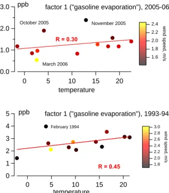
Gasoline evaporation

Modeled gasoline evaporation sources (factor 1) in 1993– 1994 and in 2005–2006 are positively correlated with tem-perature R=0.45 and R=0.30 (Fig. 7), respectively, while the other factors (related to road traffic) show a different sea-sonal behavior, typically anti- or uncorrelated with temper-ature. In several cases, positive deviations from the linear regression slope (scores vs. temperature) coincide with low wind speed (Fig. 7), which is indicative for thermal

inver-100 80 60 40 20 0 ethane ethene

propane propene ethyne isobutane n-butane

isopentane n-pentane

S-isohexanes

n-hexane benzene toluene

non-solvents potential organic solvents

Explained variance [%] by factor 2a and factor 2b (1993-1994)

Fig. 6. Explained variance by factor 2a (“non-toluene solvents”)

and factor 2b (“toluene”) for the 13 hydrocarbons considered for this study. Non-solvents comprise C2–C4 hydrocarbons ethane, ethene, propane, propene, ethyne, isobutene and butane. C5–C7 hy-drocrabons isopentane, n-pentane, S-isohexanes, n-hexane, benzene and toluene are potential organic solvents. S-isohexanes includes 2-methylpentane and 3-2-methylpentane

sions and pollutant accumulation (e.g. in February 1994, Oc-tober 2005, and November 2005). This general dependence suggests that factor 1 in both data sets represents gasoline re-lease via evaporation, during cold starts and re-fueling rather than by warm-phase combustion. A positive correlation with temperature might also be due to a combustion-related gaso-line source that is active in summer (e.g. from ship traffic or from engines used at road works), but is rather unlikely due to relatively low correlations with the inorganic combustion tracers (Table 4).

The comparison of the PMF calculated gasoline factor with methyl-tert-buthyl-ether (MTBE) measured during two campaigns in 2005–2006 (Legreid et al., 2007b) provides further evidence for an evaporative gasoline loss. Poulopou-los and PhilippopouPoulopou-los (2000) reported MTBE exhaust emis-sion particularly during cold start and from evaporation. This is in agreement with other studies (e.g. MEF, 2001). Further, MTBE is neither synthesized in Switzerland nor formed sec-ondarily in the atmosphere, but exclusively used as a gaso-line additive with concentrations between 2% and 8% per volume (BAFU, 2002). The gasoline factor is strongly corre-lated with MTBE in summer as well as in winter (Fig. 8) and, therefore, likely represents evaporative gasoline loss and cold start phases. The slightly higher correlation found in sum-mer (R=0.81) compared to winter (R=0.71) is most probably due to larger temperature differences between day and night, which determine the amplitude of evaporative gasoline loss. Gasoline and diesel fuel combustion

As for gasoline evaporation, factors representing fuel com-bustion were also found in both data sets (factor 6). They ex-hibit a bimodal daily cycle with peaks in the morning around

5 4 3 2 1 0 20 15 10 5 0 3.0 2.8 2.6 2.4 2.2 2.0 1.8 wind speed, m/s February 1994

factor 1 ("gasoline evaporation"), 1993-94

temperature R = 0.45 ppb 3.0 2.0 1.0 0.0 20 15 10 5 0 October 2005 March 2006 R = 0.30

factor 1 ("gasoline evaporation"), 2005-06

temperature November 2005 ppb 2.4 2.2 2.0 1.8 1.6 wind speed, m/s

Fig. 7. Monthly median scores of the gasoline factors (PMF

re-trieved), temperature and wind speed for the years 1993–1994 (bottom) and 2005–2006 (top). Positive deviations from the regression slope vs. temperature represent months characterized by frequent thermal inversions: February 1994, October 2005, and January 2006. Regression slopes (coefficient value ±1 σ ): 0.043±0.027 (1993–1994, n=12) and 0.018±0.018 (2005–2006,

n=12) for the monthly values presented above, 0.116±0.006 (1993–

1994, n=7606) and 0.032±0.002 (2005–2006, n=8912) for all data points.

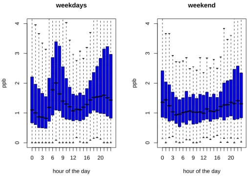
07:00 a.m. and in the evening at 09:00 p.m. in both data sets, as shown in Fig. 9 for the recent case (2005–2006). Typ-ically, this temporal behavior is much more prominent on working days. A very similar pattern as found here was also reported for organic aerosol emissions from incomplete fuel combustion and NOx at Zurich-Kaserne (Lanz et al., 2007). The pronounced diurnal variation of this factor during weekdays indicates that other fossil fuel combustion sources (e.g., off-road vehicles and machines) have a minor impor-tance at this site. On the other hand, the strong dependence of the day of the week further supports findings based on the hydrocarbon fingerprint of this factor (Sect. 3.4), namely that diesel exhaust is a major contributor. A large fraction (∼66%, deduced from BAFU, 2000) of diesel-related total hydrocarbons in 2000 was caused by the heavy-duty fleet (transport of goods), which is not allowed to drive on week-ends in Switzerland. Also commuter traffic is at a minimum, but the share of diesel passenger cars was and is still paratively low in Switzerland (∼10%, HBEFA, 2004) com-pared to its neighboring states, as diesel taxes are relatively

Winter: 19 December 2005 - 1 February 2006 (n=594)

Summer: 1 July - 1 August 2005 (n=340)

0.6 0.4 0.2 11.07.2005 21.07.2005 31.07.2005 6 5 4 3 2 1 0 R = 0.81 ppb ppb 0.4 0.3 0.2 0.1 27.12.2005 06.01.2006 16.01.2006 26.01.2006 8 6 4 2 0 factor 1 ("gasoline evaporation") MTBE (measured)

R = 0.71

ppb ppb

Fig. 8. Scores of factor 1 (“gasoline”; black) versus measured

methyl-tert-butyl-ether (MTBE, red) for the summer 2005 (bottom) and winter 2005/2006 (top). MTBE was measured at the same time during two campaigns.

high and petroleum taxes rather low (Kunert and Kuhfeld, 2007). Note that the same diurnal behavior was also found for other factors (e.g. solvents use; Sect. 3.5.4), but neither for ethane and propane sources (Sect. 3.5.3) nor for wood burning (Sect. 3.5.2).

Other traffic-related sources

In 1993–1994, a similar factor to the gasoline evaporation and cold start source can be found (see Sect. 3.4.2), but due to the absence in 2005–2006 we hypothesize that this fac-tor represents gasoline combustion by cars without catalytic converters (factor 7, 1993–1994). Recall that the fraction of non-catalyst vehicles was still in the order of one third of all passenger cars in the early 1990s (Sect. 3.4.2) and emissions were higher than from engines equipped with a catalytic con-verter. Today, this fraction is negligible: a large decrease in t-NMVOC (as well as in NOx) was found in measurements of the Gubrist tunnel, which is located in the surroundings of Zurich (Colberg et al., 2005, Legreid et al., 2007a). Such tun-nel studies do not cover cold start emissions and the large de-crease was mainly attributed to the introduction of catalytic converters in the Swiss gasoline fleet. Therefore, no such factor could be resolved for the recently measured hydrocar-bons (2005–2006). We will label this factor “earlier traffic source”.

3.5.2 Wood burning

Unlike the evaporative gasoline loss described in Sect. 3.5.1, factors representing wood burning activities are typically anti-correlated with temperature (i.e. increased domes-tic heating when outdoor temperatures are lower) and

0 3 6 9 12 16 20 0 1 2 3 4 weekdays

hour of the day

ppb 0 3 6 9 12 16 20 0 1 2 3 4 weekend

hour of the day

ppb

Fig. 9. Hourly boxplots of the modeled “fuel combustion” factor (2005–2006) for weekdays (Monday–Friday; left) and weekends (Saturday

and Sunday; right).

accumulate strongest during winter months that frequently are associated with temperature inversions (November to February; Ruffieux et al., 2006) (Fig. 10). In fact, the wood burning (and ethane) contributions were comparatively high in November 1993 and February 1994, which can be ex-plained by low wind speed and temperature that prevailed during those months. For the wood burning source strengths, no significant difference between daily emission pattern on working and non-working days can be observed (also when the data of different seasons are analyzed separately). It has been suspected that wood is mainly used for private, supple-mentary room heating in winter (Lanz et al., 2008), which is not connected to working days.

It is interesting to note that the modeled maximum wood burning emission in winter (January 2006 vs. February 1994) decreased by less than a factor 1.5, while modeled annual emissions decreased by a factor of 2.0. Therefore, the de-crease of wood burning VOCs mainly results from reduced emissions in spring, summer, and autumn, potentially caused by changes in agricultural and horticultural management. 3.5.3 Ethane and propane sources

The ethane (2005–2006) and propane (1993–1994 and 2005– 2006) dominated factors generally exhibit a diurnal pattern different from other hydrocarbon sources, i.e. a bimodal daily cycle with maxima in the morning and late evening as found for fuel combustion (Sect. 3.5.1). In contrast, the diurnal patterns of the propane and ethane dominated fac-tors are generally characterized by an early morning

max-imum and a mid-afternoon minmax-imum, which was observed for measured methane as well. This behavior is shown for the 1993–1994 and 2005–2006 data in Fig. 11. Generally such a behavior is interpreted as accumulation during the night under a shallow inversion layer followed by reducing con-centrations as the boundary layer expands during the morn-ing and early afternoon (e.g. Derwent et al., 2000). Con-centrations are therefore highest when the boundary layer is smallest and lowest when the boundary layer is highest. This implies that these emission rates must be reasonably constant between day and night. The medians between mid-night and 04:00 a.m. (small traffic contribution) increase lin-early for the propane and ethane factor, but also for mea-sured methane in 2005–2006 (Fig. 11): an emission ratio for methane:“ethane”:“propane” of about 180:3:1 can be de-duced. Natural gas leakage is an obvious candidate for the main urban source of these hydrocarbons, especially as a compositional ratio (per volume) of 190(±129):3.7(±0.8):1 (methane:ethane:propane) can be deduced for transported natural gas in Zurich (Erdgas Ostschweiz AG, Zurich, 2005/2006, unpublished data). These large uncertainties mainly reflect the variable gas mix, and might explain why gas leakage is represented by two factors rather than by one factor. Natural gas consumption in [GWh] increased by 50% from 1992 to 2005 in Switzerland; it is typically more than four times higher in winter than in summer, which would explain its correlation with SO2. For the early data (1993– 1994), the presence of ethyne (Fig. 6) and a weak bimodal daily cycle (Fig. 11) point to the possibility that the ethane

20 15 10 5 0 12 10 8 6 4 2 3.0 2.8 2.6 2.4 2.2 2.0 1.8 1.6 12 10 8 6 4 2 10 8 6 4 2 "ethane" 1993-94 (factor 4) 2005-06 (2.5 • factor 4) temperature, °C 1993-94 2005-06

Month of the year ppb wind speed, m/s 1993-94 2005-06 "wood burning" 1993-94 (factor 5) 2005-06 (2.5 • factor 5)

Fig. 10. Factors representing wood burning (brown) and the

“ethane” factors (orange), measured temperature (red) and wind speed (green) as monthly medians in 1993–1994 and 2005–2006 (dashed).

factor was then also influenced by incomplete combustion, possibly from residential (gas or oil) heating due to its yearly trend similar to that of wood burning (Fig. 10). It finally has to be noticed that factors 3 and 4 in both data sets predomi-nantly explain the variability (>60%) of ethane and propane, respectively. The normalized loadings of other hydrocarbons than ethane and propane (e.g. butane in the “propane” factor from 2005–2006) do not represent their explained variability, but are, in other words, partially floating species within the mentioned factors.

Due to their relatively long atmospheric lifetimes (days to weeks), propane and ethane (also from other sources than gas leakage) tend to accumulate in the air. Therefore, we can not completely rule out that the factors “ethane” and “propane” may also represent aged VOC emissions as sus-pected by Buzcu and Fraser (2006). However, given the seasonal and diurnal patterns of those factors (Fig. 10 and Fig. 11) the contribution of processed VOC source emis-sions can not be of a major importance. For aged and sec-ondary organic aerosols (SOA) with similar lifetimes (days to weeks as the considered hydrocarbons) Lanz et al. (2007 and 2008) have calculated increasing concentrations in the early after-noon (due to elevated photochemical activity) and only a slight enhancement of their mean concentrations in the winter (5.3 µg m−3) compared to summer (4.4 µg m−3), as stronger accumulation and partitioning of volatile precur-sors outweigh less solar radiation in wintertime (Strader et al., 1999). Furthermore, ethane and propane concentrations reported for European background air exhibit different levels and time trends than the factors as calculated for the urban site here (also see Sect. 4). Firstly, the ethane factors, as an

example, showed 3–8 times higher concentrations than re-ported for ethane in Finnish background air (Hakola et al., 2006). Note that ethane is decomposed faster at mid lati-tudes than in Polar air (due to the temperature dependence of the ethane-OH reaction rate constant and [OH] levels). Sec-ondly, we estimated that ethane and propane dominated fac-tors, most likely representing natural gas leakage, slightly decreased by a factor of 1.3 from 1993–1994 to 2005–2006, whereas background ethane and propane showed increasing trends between 1994 and 2003 (Hakola et al., 2006). We therefore conclude again that the hydrocarbon concentrations measured at the urban background of Zurich-Kaserne can not be significantly influenced by aged background air (also see Sects. 2.2.2 and 3.3.2).

3.5.4 Solvent usage

Acetates (belonging to the class of OVOCs) are commonly used solvents in industry (Legreid et al., 2007b). Also Niedo-jadlo et al. (2007) measured elevated acetate concentrations close to industries in Wuppertal (Germany). A strong corre-lation was found between the sum of acetates (methyl-, ethyl, and butyl-) measured during two campaigns in 2005–2006 and the calculated solvent factor for 2005–2006 (Fig. 12). Lower correlation of acetates in summertime (R=0.61) than in wintertime (R=0.70) is possibly due to secondary forma-tion of acetates in the atmosphere, which is triggered by pho-tochemistry. Further note that factor 2 was derived for two years of data; it nevertheless seems representative of weekly to daily variability of this hydrocarbon source.

3.6 Source contributions

Average source contributions as absolute concentrations [ppb] and relative [%] to the total mixing ratio of the 13 hy-drocarbons were calculated for both data sets and summa-rized in Table 5.

3.6.1 Representativeness of the 13 hydrocarbons

The concentrations of the 13 hydrocarbons considered in this study accounted on average for 80–90% ppbC/ppbC of the sum of all 22 NMHC species measured at this site since 2005. Aromatic C8hydrocarbons (m,p-xylene, o-xylene, and ethyl-benzene) represent a major fraction of that difference, ac-counting for more than 6% of the total concentration [ppb] of the 22 NMHCs. They were not measured continuously in 1993 and 1994. A PMF analysis of the extended data set (2005–2006; comp. Sect. 3.3.1) revealed that those latter aromatics will be attributed to solvent use (60%), fuel com-bustion (30%), gasoline evaporation (5%), and wood burning (3%).

The 22 NMHCs plus the 22 oxidized VOCs compounds (∼20%; measured during four seasonal campaigns in 2005 and 2006, Sect. 2.1.2) sum up to 78%-85% of the t-NMVOC concentrations (in ppbC) determined by FID. For the earlier

0 3 6 9 12 16 20 0 2 4 6 8 factor 4 (’ethane’): 1993−94

Hour of the day

ppb 0 3 6 9 12 16 20 0 1 2 3 4 5 factor 3 (’propane’): 1993−94

Hour of the day

ppb 0 3 6 9 12 16 20 1.7 1.8 1.9 2.0 2.1 2.2 2.3 2.4 methane (measured): 1993−94

Hour of the day

ppm 0 3 6 9 12 16 20 0 2 4 6 8 factor 4 (’ethane’): 2005−06

Hour of the day

ppb 0 3 6 9 12 16 20 0 1 2 3 4 5 factor 3 (’propane’): 2005−06

Hour of the day

ppb 0 3 6 9 12 16 20 1.7 1.8 1.9 2.0 2.1 2.2 2.3 2.4 methane (measured): 2005−06

Hour of the day

ppm

Fig. 11. Hourly boxplots of factors dominated by ethane (left) and propane (middle), measured methane (right) for 1993–1994 (top) and

2005–2006 (bottom).

data (1993–1994), the 18 NMHCs (measured by GC-FID) accounted for 63% of t-NMVOC (FID) on average. In the latter campaign, OVOCs were not determined directly, but via the subtraction of non-oxidized NMHCs (retrieved by GC-FID and measurements of passive samplers) from the t-NMVOC signal we can say that about 20% or less VOCs were oxidized. Unlike the hydrocarbons used in this study, most OVOCs can be both directly released into the atmo-sphere or formed there secondarily. Furthermore they can be of anthropogenic as well as biogenic origin (Legreid et al., 2007b). We therefore conclude that the 13 hydrocarbons used in the present study are representative for primary and anthropogenic hydrocarbon emissions in Zurich.

3.7 Hydrocarbon emission trends (1993–1994 vs. 2005– 2006)

For most hydrocarbon sources (road traffic, solvent use, and wood combustion) decreasing contributions by a factor of 2–3 between 1993–1994 and 2005–2006 were modeled (Ta-ble 5 and Fig. 13). This trend is also reflected by the de-cline of t-NMVOC measurements (Fig. 1) and vice versa. However, for ethane and propane sources (mainly natural gas leakage), no such strong negative trend was found. In con-trast, propane and ethane sources only decreased by a fac-tor of 1.3 (but its consumption increased about 1.5 times). In Switzerland, steering taxes of about 2 Euro per kg VOC were enforced in 1998. They are based on a black list of about 70 VOC species (e.g. toluene) or VOC classes (e.g. aromatic mixtures). Unlike most VOCs used in or as solvents, propane and ethane are not part of the black list (VOCV, 1997). The relatively constant ethane and propane

Table 5. Summary of hydrocarbon (sum of 13 C2through C7species) source apportionments for both periods 1993–1994 and 2005–2006 and all factors. Factor grouping to classes of hydrocarbon sources.

mean rel. contr. median contr. 1. quart. 3. quart. mean conc.

[%] [%] [%] [%] [ppb]

PMF factors 2005–2006

factor 1 “gasoline evaporation” 13 13 8 18 1.7

factor 2 “solvents” 20 20 13 27 2.7

factor 3 “propane” 14 14 10 18 1.9

factor 4 “ethane” 21 19 13 27 2.7

factor 5 “wood burning” 16 15 10 20 2.1

factor 6 “fuel combustion” 13 13 9 17 1.7

total explained mass conc. 97%

average total conc. 13.2 ppb

1993–1994

factor 1 “gasoline evaporation” 15 13 9 18 3.7

factor 2a “non-toluene solvents” 10 9 8 11 2.4

factor 2b “toluene” 8 7 5 10 2.0

factor 3 “propane” 8 7 4 10 1.9

factor 4 “ethane” 17 15 9 23 4.1

factor 5 “wood burning” 17 17 12 22 4.2

factor 6 “fuel combustion” 11 11 8 13 2.6

factor 7 “earlier traffic source” 15 14 9 19 3.6

total explained mass conc. 99%

average total conc. 24.8 ppb

Source groups 2005–2006

factor 1, 6 road traffic 26 26 20 33 3.5

factor 2 solvent use 20 20 13 27 2.7

factor 5 wood burning 16 15 10 20 2.1

factor 3, 4 gas leakage 35 33 25 43 4.6

1993–1994

factor 1, 6, 7 road traffic 40 38 26 50 9.9

factor 2a, 2b solvent use 18 17 13 21 4.4

factor 5 wood burning 17 17 12 22 4.2

factor 3, 4 gas leakage 24 22 13 33 6.0

levels from gas leakage are in agreement with relatively con-stant methane concentrations measured in 1993–1994 and 2005–2006: ethane (1%–6%) and propane (∼1%) are minor components of natural gas, which predominantly consists of methane (>90%). On the other hand, methane has a life-time of years and is emitted by other sources as well (e.g. in-complete combustion of fossil and non-fossil materials) and therefore no perfect correlation can be expected.

3.7.1 Traffic-related sources and solvent use

The EMEP (Cooperative Programme for Monitoring and Evaluation of the Long-range Transmission of Air Pollutants in Europe) emission inventory for Switzerland (1993 versus 2004) suggests that the most dominant VOC sources, i.e. sol-vent use (115×106kg or 55% of t-NMVOC in 1993) and

road transport (63×106kg or 30% of t-NMVOC in 1993) de-creased by a factor of two and three, respectively (Vestreng et al., 2006). Roughly the same relative decrease for road traffic and solvent use can be deduced from the data pre-sented in Table 5 and Fig. 13. However, we estimate that traffic is still an important VOC emission source accounting on average for 40% ppb/ppb (1993–1994) and 26% ppb/ppb (2005–2006) of the total mixing ratio of the 13 hydrocar-bons (or 43% µg m−3/µg m−3 and 27% µg m−3/µg m−3, respectively). In contrast, solvent usage contributed on av-erage only to about 20% ppb/ppb (and about 5%–10% more if based on µg m−3/µg m−3) of the ambient levels of the 13 hydrocarbons measured at Zurich-Kaserne. For the 1993– 1994 data Staehelin et al. (2001) (details in Sect. 3.4.2) have also found that road traffic contributes at least twice as much to ambient hydrocarbon concentrations than solvents, which