Modelling the global tropospheric ozone budget: exploring the variability in current models

HAL Id: hal-00296234

https://hal.archives-ouvertes.fr/hal-00296234

Submitted on 21 May 2007

HAL is a multi-disciplinary open access

archive for the deposit and dissemination of

sci-entific research documents, whether they are

pub-lished or not. The documents may come from

teaching and research institutions in France or

abroad, or from public or private research centers.

L’archive ouverte pluridisciplinaire HAL, est

destinée au dépôt et à la diffusion de documents

scientifiques de niveau recherche, publiés ou non,

émanant des établissements d’enseignement et de

recherche français ou étrangers, des laboratoires

publics ou privés.

exploring the variability in current models

O. Wild

To cite this version:

O. Wild. Modelling the global tropospheric ozone budget: exploring the variability in current models.

Atmospheric Chemistry and Physics, European Geosciences Union, 2007, 7 (10), pp.2643-2660.

�hal-00296234�

© Author(s) 2007. This work is licensed under a Creative Commons License.

Chemistry

and Physics

Modelling the global tropospheric ozone budget: exploring the

variability in current models

O. Wild

Frontier Research Center for Global Change, JAMSTEC, Yokohama, Japan now at: Centre for Atmospheric Science, University of Cambridge, UK

Received: 11 January 2007 – Published in Atmos. Chem. Phys. Discuss.: 8 February 2007 Revised: 4 May 2007 – Accepted: 4 May 2007 – Published: 21 May 2007

Abstract. What are the largest uncertainties in modelling ozone in the troposphere, and how do they affect the cal-culated ozone budget? Published chemistry-transport model studies of tropospheric ozone differ significantly in their conclusions regarding the importance of the key processes controlling the ozone budget: influx from the stratosphere, chemical processing and surface deposition. This study sur-veys ozone budgets from previous studies and demonstrates that about two thirds of the increase in ozone production seen between early assessments and more recent model intercom-parisons can be accounted for by increased precursor emis-sions. Model studies using recent estimates of emissions compare better with ozonesonde measurements than stud-ies using older data, and the tropospheric burden of ozone is closer to that derived here from measurement climatolo-gies, 335±10 Tg. However, differences between individual model studies remain large and cannot be explained by sur-face precursor emissions alone; cross-tropopause transport, wet and dry deposition, humidity, and lightning also make large contributions. The importance of these processes is ex-amined here using a chemistry-transport model to investigate the sensitivity of the calculated ozone budget to different as-sumptions about emissions, physical processes, meteorology and model resolution. The budget is particularly sensitive to the magnitude and location of lightning NOxemissions, which remain poorly constrained; the 3–8 TgN/yr range in recent model studies may account for a 10% difference in tropospheric ozone burden and a 1.4 year difference in CH4 lifetime. Differences in humidity and dry deposition account for some of the variability in ozone abundance and loss seen in previous studies, with smaller contributions from wet de-position and stratospheric influx. At coarse model resolu-tions stratospheric influx is systematically overestimated and dry deposition is underestimated; these differences are 5–8%

Correspondence to: O. Wild

(oliver.wild@atm.ch.cam.ac.uk)

at the 300–600 km grid-scales investigated here, similar in magnitude to the changes induced by interannual variabil-ity in meteorology. However, a large proportion of the vari-ability between models remains unexplained, suggesting that differences in chemical mechanisms and dynamical schemes have a large impact on the calculated ozone budget, and these should be the target of future model intercomparisons.

1 Introduction

Ozone is an important greenhouse gas, a major component of photochemical smog, and the primary source of hydroxyl radicals which control the oxidizing capacity of the tropo-sphere (e.g., Prather and Ehhalt, 2001). The abundance of O3in the troposphere is controlled by transport from the O3 -rich stratosphere, by chemical production following the ox-idation of hydrocarbons and CO in the presence of nitrogen oxides (NOx) and by removal via chemical destruction or dry deposition. The magnitudes of these sources and sinks have not been reliably quantified, and observational constraints on them remain poor. The chemical lifetime of O3 in the tro-posphere, typically days to weeks, is similar in magnitude to the dynamical timescales for transport and mixing, and thus the factors controlling O3are not easily separable. The net effects of chemical processing are dependent on the bal-ance between large production and destruction terms which dominate in different regions of the troposphere, and the im-portance of stratosphere-troposphere exchange (STE) is sim-ilarly dependent on the balance between downward transport of O3 from the stratosphere, mostly at mid-latitudes, and a smaller upward flux in tropical regions. The equilibrium between these chemical and dynamical fluxes constitutes a buffering of tropospheric O3, and poor estimates of one or more of these governing processes may be masked by read-justment of the others so that the abundance of O3 in the troposphere is not greatly affected. However, a quantitative

understanding of the processes controlling the production, redistribution and fate of O3 in the troposphere is required before a reliable assessment can be made of how O3may re-spond to changes in anthropogenic emissions of trace gases or global climate.

Global chemistry-transport models (CTMs) that simulate the chemical and dynamical processes controlling O3 pro-vide a self-consistent estimate of the key budget terms. Most CTMs can reproduce the seasonality and distribution of tro-pospheric O3 measured by ozonesondes in a climatological sense, but assessments of the relative importance of the con-trolling processes vary widely (Prather and Ehhalt, 2001). Recent model intercomparison studies estimate a net O3 in-flux of 550±170 Tg/yr from the stratosphere and a surface re-moval of 1000±200 Tg/yr by dry deposition, with net chem-ical production making up the balance of 450±300 Tg/yr (Stevenson et al., 2006). However, there are large differences between individual model studies in the importance of these terms reflecting differences in their treatments of chemical and dynamical processes. These differences highlight signif-icant imperfections in our current understanding of the key factors involved (e.g., in the magnitude and distribution of emissions, chemical processing, and convection) and in their numerical representation at computationally-tractable tem-poral and spatial scales. CTMs are typically focussed on global-scale issues such as attribution of climate impacts due to changing patterns of fossil fuel combustion (Gauss et al., 2003; Dentener et al., 2006a), or assessment of the policy impacts of intercontinental transport of oxidants on air qual-ity (e.g., Holloway et al., 2003). Many of the chemical and dynamical processes controlling O3 in the troposphere oc-cur at much smaller temporal and spatial scales than can be resolved in these models, and thus important processes are parameterized, introducing additional uncertainty. Never-theless, improved understanding of the interactions between tropospheric composition and climate, and in particular of how changes in climate may affect the sources and fate of tropospheric O3, requires that the principal terms in the O3 budget can be quantified in a reliable and consistent way so that the sensitivity of the budget to changes in transport, con-vection, chemistry and deposition can be evaluated reliably. Recent model intercomparison exercises have suggested that this may not currently be the case (Prather and Ehhalt, 2001; Stevenson et al., 2006).

The aims of this paper are to explore the differences seen in previous model estimates of the source and fate of tro-pospheric O3, and to investigate to what extent these arise from the use of different input conditions or from differences in model formulation. Differences in precursor emissions or meteorological data may mask the more subtle differences that reflect improved scientific understanding or deficiencies in process representation. Identifying the source of these dif-ferences is important for reducing the uncertainty in the mod-elled response of tropospheric O3to applied changes and for interpreting the results of multi-model “ensemble” studies.

The sensitivity of the budget terms to key model processes is explored here in a consistent way with a single model. Section 2 reviews tropospheric O3 budgets from published studies and highlights the origins of some of the differences between them. Section 3 describes the limited observational constraints on the O3 budget. Section 4 then examines the sensitivity of the budget terms to emissions, meteorology, and key physical processes and interprets the variability seen in previous studies in light of these results. The implications of the results for future model intercomparison studies are outlined in Sect. 5.

2 Tropospheric ozone budgets in global models

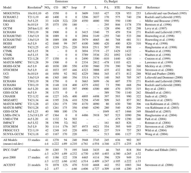
A comparison of O3 budgets from published global model studies is presented in Table 1. The studies are ordered chronologically by publication date, and statistics from ear-lier studies summarised in the Intergovernmental Panel on Climate Change (IPCC) Third Assessment Report (TAR) (Prather and Ehhalt, 2001) are compared with those pub-lished since 2000 to show how the calculated O3budget has evolved. There are large differences in the key terms be-tween individual model studies: STE fluxes vary by a factor of four (340–1440 Tg/yr), deposition fluxes vary by almost a factor of three (530–1470 Tg/yr), and gross chemical pro-duction varies by a factor of two (2330–5260 Tg/yr). The tropospheric burden of O3varies between 240 and 380 Tg. However, these studies vary widely in their precursor emis-sions and in model formulation and resolution. Many of the pioneering early studies used simplified chemistry schemes omitting oxidation of non-methane hydrocarbons (NMHC), and a number of them had unreasonably high estimates of stratospheric influx; compensation between the key terms in the budget leads several studies to conclude that the tropo-sphere is a net chemical sink of O3. Recent studies have benefited from more detailed chemical schemes, improved understanding of the emissions of key precursor species, and better quality meteorological data at higher spatial resolu-tion. This has reduced the variability in independent stud-ies published since 2000 compared with those surveyed in the IPCC-TAR, but the 1σ variability remains large: STE 530±100 Tg/yr, net production 400±250 Tg/yr, and deposi-tion 950±220 Tg/yr. It is not clear how much of this vari-ability is due to the use of different input data (e.g., emis-sions or meteorological data) and how much is down to different model treatments of the key processes involved. These studies have typically used their own definitions of the tropopause and of the chemical fluxes constituting O3 pro-duction, making direct comparison of O3burdens, lifetimes and tendencies particularly difficult.

A recent model intercomparison coordinated by the Euro-pean Union project Atmospheric Composition Change: the European Network of Excellence (ACCENT) involved many of the models shown in Table 1 and aimed to reduce these

Table 1. Global ozone budgets from published CTM studiesa.

Emissions O3Budget

Model Resolutionb NOx CO HCc Isop P L P-L STE Dep Burd Reference

MOGUNTIA 10x10 L10 45 1550 0 0 3609 3183 427 528 953 253 Lelieveld and van Dorland (1995)

ECHAM3.2 T21 L19 40 1400 0 0 3206 3037 170 575 740 236 Roelofs and Lelieveld (1995)

IMAGES 5x5 L25 33 1428 322t 220 4550 4000 550 550 1100 – M¨uller and Brasseur (1995)

UIO 8x10 L9 35 1575 150 180 – – 295 846 1178 370 Berntsen et al. (1996)

GCTM 265 km L11 40 – 0 0 – – 128 696 825 298 Levy et al. (1997)

ECHAM4 T30 L19 38 1900 0 0 3415 3340 75 459 534 271 Roelofs and Lelieveld (1997)

ECHAM/TM3 3.8x5 L9 38 1089 0 0 2894 3149 –255 740 533 266 Houweling et al. (1998)

ECHAM/TM3 3.8x5 L9 38 1089 108 400 3979 4065 -86 768 681 311 Houweling et al. (1998)

HGISS 4x5 L9 42 1040 99 597 4100 3680 420 400 820 310 Wang et al. (1998)

MOZART T42 L25 43 1219 251t 220 3018 2511 507 391 898 – Hauglustaine et al. (1998)

CTMK 4x5 L15 38 – 0 0 3694 3719 –27 1429 1432 – Wauben et al. (1998)

CTMK 4x5 L15 38 – 0 0 3789 3536 252 1092 1363 – Wauben et al. (1998)

MATCH T21 L28 37 1350 0 0 2490 3300 –810 1440 620 – Crutzen et al. (1999)

MATCH-MPIC T63 L28 39 1500 0 0 2334 2812 –478 1103 621 – Lawrence et al. (1999)

HGISS-GCM 4x5 L9 40 1030 100 550 4330 3960 370 390 760 360 Mickley et al. (1999)

STOCHEM 5x5 L9 41 1033 197 446 4323 3888 435 432 862 316 Stevenson et al. (2000)

UCI 8x10 L9 44 1050 92 502 4229 3884 345 473 812 288 Wild and Prather (2000)

TM3 3.8x5 L9 46 1365 160 356 3314 3174 140 565 705 347 Lelieveld and Dentener (2000)

ECHAM4 T30 L19 38 1750 0 0 3663 3699 -36 607 570 271 Roelofs and Lelieveld (2000)

ECHAM4 T30 L19 38 1148 118 400 4375 4302 73 590 668 294 Roelofs and Lelieveld (2000)

GEOS-CHEM 4x5 L20 46 1043 103 397 4900 4300 600 470 1070 315 Bey et al. (2001)

GISS-GCM 4x5 L9 38 1175 0 0 – – 389 750 1140 262 Shindell et al. (2001)

CHASER T21 L32 44 1227 145t 400 4895 4498 397 593 990 322 Sudo et al. (2002)

MOZART2 T42 L34 44 1195 218t 410 5258 4749 509 343 857 362 Horowitz et al. (2003)

MATCH-MPIC T21 L28 43 1261 175 350 4170 4090 80 630 700 306 von Kuhlmann et al. (2003)

MATCH-MPIC T63 L28 43 1261 175 350 4560 4290 280 540 820 294 von Kuhlmann et al. (2003)

GISS-GCM 4x5 L23 40 988 100 176 – – 1049 417 1466 349 Shindell et al. (2003)

LMDz-INCA 2.5x3.8 L19 47 1364 0 0 4486 3918 567 523 1090 296 Hauglustaine et al. (2004)

UMD-CTM 4x5 L20 41 1132 54 503 – – – 479 1290 340 Park et al. (2004)

IMPACT 4x5 L52 38 1398 52t 502 – – 161 663 826 – Rotman et al. (2004)

STOCHEM 5x5 L9 50 1114 179t 507 4975 4421 554 395 949 273 Stevenson et al. (2004)

FRSGC/UCI T21 L19 42 1248 143 220 4091 3854 237 519 757 283 Wild et al. (2004)

SUNYA-GCCM T42 L18 43 1167 170 220 – – 513 606 1127 376 Wong et al. (2004)

All Models 33 studies 41 1270 94 240 3948 3745 245 636 902 307

(mean±std.dev) ±4 ±222 ±89 ±210 ±761 ±554 ±346 ±273 ±255 ±38

IPCC-TARd 12 studies 39 1285 75 195 3448 3435 46 765 818 304 Prather and Ehhalt (2001)

±3 ±293 ±89 ±232 ±730 ±505 ±403 ±380 ±265 ±32

post-2000 17 studies 43 1186 122 338 4465 4114 396 529 949 314

±3 ±122 ±66 ±162 ±514 ±409 ±247 ±105 ±222 ±33

ACCENT 21 models 51 1078 125t 470 5110 4668 442 552 1003 344 Stevenson et al. (2006)

±2 ±57 – ±66 ±606 ±727 ±309 ±168 ±200 ±39

a_{Emissions and budgets are in Tg yr}−1_{(TgN yr}−1_{for NOxand TgC yr}−1_{for hydrocarbons); dashes indicate budget data unavailable.}

b_{Resolution in degrees (latitude by longitude) and number of model levels; spectral truncations of T21, T30, T42 and T63 are used to label}

Gaussian grids with approximate resolutions of 5.6◦, 3.8◦, 2.8◦and 1.9◦respectively.

c_{Non-methane hydrocarbons excluding isoprene and terpenes; t label indicates terpenes also emitted (an additional 100–170 TgC yr−1).}

d_{Selected studies published before 2000 shown in Table 4.12 of the IPCC Third Assessment Report, with the entry for Wauben et al. (1998)}

corrected.

uncertainties by constraining fossil fuel precursor emissions and applying consistent tropopause diagnostics across all participating models (Dentener et al., 2006a; Stevenson et al., 2006). The budget terms calculated in this study were higher than those from previous studies, and the variability in the

terms was also larger, despite the more tightly constrained conditions. In particular, there is an increase in gross produc-tion between the IPCC-TAR (3450 Tg/yr), studies published since 2000 (4470 Tg/yr) and the ACCENT intercomparison (5110 Tg/yr), which is accompanied by a 10% increase in

30 35 40 45 50 55 NO_x Emissions /Tg(N)/yr 0 1000 2000 3000 4000 5000 6000 7000 O3 Production, P(O 3 ) /Tg/yr 0 100 200 300 400 500 600 700

Isoprene Emissions /Tg(C)/yr 0 1000 2000 3000 4000 5000 6000 7000 ACCENT Studies

CTM from Table 1 (with NMHC) CTM from Table 1 (w/o NMHC)

NO

Isoprene

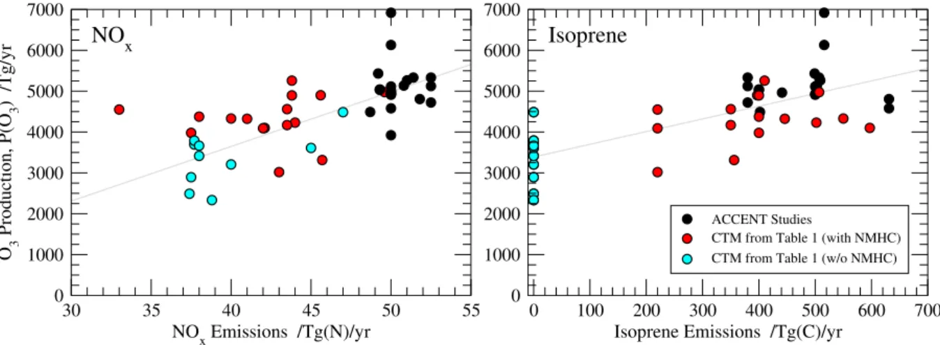
Fig. 1. Relationship between gross O3 production, P(O3), and precursor emissions for the model studies described in Table 1 with and

without hydrocarbon oxidation and for the ACCENT model intercomparison studies described in Stevenson et al. (2006).

O3burden, a 20% increase in deposition, and a drop in the tropospheric lifetime of O3from 24 to 22 days. Higher esti-mates of precursor emissions make a substantial contribution to the increased production, as noted in regression analyses by Wu et al. (2007), and largely reflect improved understand-ing of NOxsources and emission factors. The sensitivity of gross O3 production to surface emissions of NOx and iso-prene (C5H8) is shown in Fig. 1 for published studies and for individual models contributing to the ACCENT intercom-parison. While the strong dependence on emissions is clear, there is a large scatter in these plots, even for the relatively well-constrained ACCENT studies. The variation in emis-sions for the ACCENT models reflects differences in natu-ral sources of NOxand isoprene which are interactive with model vegetation and meteorology in many of the models. The scatter indicates that other factors have an important in-fluence on the budget. A major goal of the present study is to investigate the effects of these processes more closely us-ing the tighter constraints imposed by application of a sus-ingle model framework, and ensuring that comparison of budget terms is fully self-consistent.

3 Constraints from observations

Of the budget terms considered here only influx of O3from the stratosphere has been adequately estimated from obser-vational data. Murphy and Fahey (1994) used observed mid-latitude N2O–O3correlations and an upward flux of N2O de-rived from a budget analysis to derive a net downward flux of O3of 450 Tg/yr, with a range of 200–870 Tg/yr. Gettel-man et al. (1997) used lower stratospheric O3measurements and calculations of the residual circulation to derive a net downward flux of 510 Tg/yr at 100 hPa (with a range of 450– 590 Tg/yr). McLinden et al. (2000) reduced the uncertainty

in the analysis of Murphy and Fahey (1994) by considering the tighter N2O–NOyand NOy–O3relationships separately, estimating a flux of 475±120 Tg/yr, and further refinements by Olsen et al. (2001) led to the best estimate currently avail-able, 550±140 Tg/yr. Most model studies published since 2000 fall within this range, and the mean influx from the ACCENT model intercomparison was 552 Tg/yr. However, this agreement masks significant differences in the magni-tude and location of cross-tropopause fluxes and in treatment of stratospheric O3, and does not constitute an independent comparison as some models apply a flux constraint through use of tuned upper boundary conditions or an artificial strato-spheric O3tracer such as Synoz (McLinden et al., 2000).

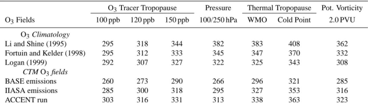
In the absence of reliable observation-based estimates of global deposition fluxes or chemical production, the best re-maining constraint is on the abundance of O3 itself. With-out details of the seasonal, geographical and altitudinal vari-ations in O3 from previous studies only a simple compari-son of the mean annual global tropospheric burden is possi-ble here. However, the tropospheric O3 burden and its de-pendence on the definition of the tropopause has not been evaluated previously. The tropospheric burden is estimated here from three different climatologies built from available ozonesonde, satellite and surface measurements, and using a number of different dynamical and thermal definitions of the tropopause, see Table 2. The climatologies were inter-polated onto a common 4◦_×5◦_{grid and integrated from the} surface to a tracer tropopause defined by a given abundance of O3(100, 120 or 150 ppb), a thermal tropopause based on a lapse rate of 2 K km−1following the WMO definition, or a dynamical tropopause based on potential vorticity (PV) us-ing the lower of the PV=2.0 surface and the tropical 380 K isentrope. For comparison, a cold-point tropopause based on the tropical temperature minimum is shown (a WMO thermal tropopause was applied in the extra-tropics), and a

stepped-Table 2. Estimated annual mean tropospheric O3burdens (in Tg) based on O3climatologies and FRSGC/UCI CTM fields with different

definitions of the tropopause.

O3Tracer Tropopause Pressure Thermal Tropopause Pot. Vorticity

O3Fields 100 ppb 120 ppb 150 ppb 100/250 hPa WMO Cold Point 2.0 PVU

O3Climatology

Li and Shine (1995) 295 318 344 382 383 408 362

Fortuin and Kelder (1998) 295 312 333 345 347 370 332

Logan (1999) 292 307 327 322 325 343 308

CTM O₃fields

BASE emissions 260 273 290 266 296 321 285

IIASA emissions 285 300 318 295 327 353 316

ACCENT run 303 316 331 313 338 363 323

isobaric tropopause typical of crude model diagnostics is also used (100 hPa in the tropics and 250 hPa poleward of 30◦). Thermal and dynamical tropopauses were calculated using monthly-mean data for year 2000 from the European Centre for Medium-Range Weather Forecasts (ECMWF); burdens calculated with 1997 data differ by less than 2 Tg (<1%). These comparisons provide only crude estimates of the true tropospheric burden, neglecting temporal or spatial varia-tions in tropopause height which may bias it high or low, but they provide a convenient benchmark against which model simulations can be compared.

Use of a tracer tropopause provides the greatest consis-tency in O3 burden for the different climatologies, as dif-ferences in O3 distribution are suppressed. This definition is the simplest to employ when comparing model studies, and based on the 150 ppb level recommended by Prather and Ehhalt (2001) suggests a tropospheric burden of 335±10 Tg for the three climatologies used here. Thermal definitions generally give higher burdens, as noted by Bethan et al. (1996), and are more sensitive to O3 differences in the tropopause region and thus more variable; the WMO lapse-rate definition gives a burden of about 352±30 Tg. Interest-ingly, the crude pressure tropopause gives very similar bur-dens to the WMO lapse-rate tropopause for all three clima-tologies used here, but note that they are quite different for typical model fields (discussed below), highlighting system-atic differences in O3distribution between modelled and cli-matological fields. The PV=2.0 dynamical tropopause gives similar burdens to the 150 ppb tracer tropopause for both model and climatological fields, and burdens are consistently lower than with the WMO lapse-rate definition.

There is considerable uncertainty in these estimates due to the sparse coverage of ozonesonde sites, but the O3 dens derived here are generally lower than the 370 Tg bur-den recommended by Prather and Ehhalt (2001). The dy-namical tropopause is represented well by the 150 ppb O3 tracer tropopause, and the mean burden of 344 Tg from the

ACCENT model intercomparison (reduced to 336 Tg after removing model outliers) (Stevenson et al., 2006) which used this tracer tropopause is in good agreement with the 335±10 Tg range estimated here from measurement clima-tology. The variability in burden for a single O3distribution based on different definitions of the tropopause is as much as ±15%, suggesting that differences in definition make an important contribution to the differences between model bur-dens shown in Table 1.

4 CTM sensitivity studies

The dependence of the calculated O3 budget on precursor emissions and on physical and meteorological variables is investigated here with a global CTM. Altering variables in-dependently allows an assessment of their contributions to the model differences seen in Table 1, and use of a single model framework ensures that the comparison of their rel-ative importance is self-consistent. A similar approach has been adopted in a recent study of uncertainties in a regional model (Mallet and Sportisse, 2006). Previous global stud-ies have focussed on the effects of individual variables, e.g., hydrocarbon oxidation (Houweling et al., 1998; Roelofs and Lelieveld, 2000; von Kuhlmann et al., 2004), STE (Wauben et al., 1998), model resolution (von Kuhlmann et al., 2003; Wild and Prather, 2006), lightning NOxemissions (Labrador et al., 2005), convection (Lawrence et al., 2003; Doherty et al., 2005), and interannual variability in meteorology (Zeng and Pyle, 2005), but have not compared their effects in a comprehensive or systematic way.

The model used here is the Frontier Research System for Global Change (FRSGC) version of the University of Cal-ifornia, Irvine (UCI) CTM described in Wild and Prather (2000) with the configuration used in Wild et al. (2004). Pieced-forecast meteorological data generated by the Eu-ropean Centre for Medium-Range Weather Forecasts Inte-grated Forecast System (ECMWF-IFS) are used to drive

1 2 3 4 5 6 7 8 9 10 11 12 10 20 30 40 50 60 70 Ozone /ppb 20 30 40 50 60 70 80 90 Ozone /ppb 1 2 3 4 5 6 7 8 9 10 11 12 20 30 40 50 60 70 80 90 Ozone /ppb 1 2 3 4 5 6 7 8 9 10 11 12 Ozonesonde Data ACCENT Run IIASA Emissions BASE Emissions 1 2 3 4 5 6 7 8 9 10 11 12

90-30oS 500 hPa 30oS-Eq 500 hPa Eq-30oN 500 hPa 30-90oN 500 hPa

30oS-Eq 250 hPa Eq-30oN 250 hPa

90-30oS 750 hPa 30oS-Eq 750 hPa Eq-30oN 750 hPa 30-90oN 750 hPa

Month of Year n=5 n=5 n=16 n=16 n=16 n=4 n=4 n=4 n=19 n=19

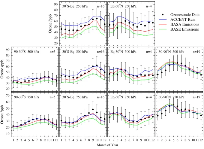
Fig. 2. Comparison of the annual cycle of O3in the FRSGC/UCI CTM with ozonesonde measurements at 750, 500 and 250 hPa averaged

over four latitude bands. Results for 3 model simulations are shown: the BASE run (green), a run with IIASA emissions (red) and a T42L37 run for year 2000 with IIASA emissions (blue). Monthly mean mixing ratios at each site are averaged over each band and are compared with model fields sampled in the same way; error bars show the average interannual standard deviation at each station. Ozonesonde data are from Logan (1999) and Thompson et al. (2003); the number of stations in each band is given by “n”.

the model. The model includes an explicit treatment of HOx/Ox/NOx chemistry and CH4 oxidation, and a lumped NMHC chemistry for the representative species butane, propene, xylene and isoprene. The 70–80 runs performed here use the same initial conditions and 8-month spin-up period, but a different variable is altered in each case to quantify its effect on the O3budget. The tropopause is di-agnosed on-line using the 120 ppb abundance of Linoz, an O3-like tracer with a linearised O3chemistry in the strato-sphere, no loss in the free troposphere and a 2-day relaxation to 20 ppb at the surface (McLinden et al., 2000). For consis-tency with other published studies, O3budget terms are diag-nosed from monthly-mean model output based on a 150 ppb O3tracer tropopause (Prather and Ehhalt, 2001; Stevenson et al., 2006). The difference in O3burden between this di-agnostic O3tropopause and the on-line Linoz tropopause is generally less than 10 Tg, about 3%. The STE flux is in-ferred as the residual term in the O3budget after accounting for the diagnosed net chemical production and deposition and the net change in burden over the year. Gross chemical

pro-duction and destruction of O3are diagnosed from the model chemistry scheme; gross destruction is based on the reac-tion fluxes of O(1D) with water vapour and of O3with HOx and alkenes, and gross production is taken as the difference between the calculated chemical O3tendency and the diag-nosed destruction rate to ensure mass consistency.

Two sets of emissions scenarios are used in these exper-iments. The base scenario (“BASE”) for NOx, CO and NMHC loosely represents 1990’s understanding, and is taken from version 2 of the EDGAR database for 1990 (Olivier et al., 1996) with isoprene emissions from Guenther et al. (1995) reduced to 220 TgC/yr following Hauglustaine et al. (1998). A second, updated scenario (“IIASA”) uses indus-trial emissions distributions from EDGAR v3.2 for 1995 (Olivier and Berdowski, 2001) scaled to the year 2000 us-ing emission data from the International Institute for Applied Systems Analysis (IIASA) (Dentener et al., 2005), as rec-ommended for the recent ACCENT model intercomparison. Biomass burning emissions from van de Werf et al. (2003) are used with this scenario, together with the full 500 TgC/yr

of isoprene emissions from Guenther et al. (1995). Lightning NOxemissions of 5 TgN/yr and CH4emissions of 550 Tg/yr are used with both these scenarios. The sensitivity studies described here use the BASE emissions unless otherwise in-dicated, and are run with 1996 meteorology at T21L19 reso-lution (5.6◦×5.6◦resolution with 19 levels).

Model runs are evaluated by comparing with ozonesonde observations from the period 1980–1993 (Logan, 1999), sup-plemented by additional data from the tropics between 1997 and 2002 (Thompson et al., 2003). Monthly interannual mean O3 mixing ratios at selected altitudes at each loca-tion are averaged over four latitude bands and compared with monthly means from model simulations sampled at the same locations, following the method of Stevenson et al. (2006), see Fig. 2. Three model scenarios are shown to illustrate the range of O3responses: the control run (BASE), a run with updated emissions (IIASA), and a run contributed to the AC-CENT intercomparison (ACAC-CENT) which used IIASA emis-sions in different model conditions (year 2000 meteorology with higher horizontal and vertical resolution, T42L37, and minor improvements to model physics described in Wild and Prather, 2006). While the magnitude and seasonality of O3 are captured reasonably well in these runs, a number of dis-crepancies clearly remain, most notably in the wintertime at Northern mid-latitudes and in the tropical upper troposphere. The difference between BASE and IIASA runs shows how changes in precursor emissions alone contribute to changes in O3; comparison with observations suggests that emissions in the BASE scenario are too low, particularly in the trop-ics. Differences between the IIASA and ACCENT runs re-flect changes in meteorology and resolution, although differ-ences in the tropical upper troposphere are influenced by the use of marginally higher lightning NOxemissions in the AC-CENT run (6.5 TgN/yr rather than 5 TgN/yr) and application of the observation-based emissions profiles of Pickering et al. (1998) in place of uniform profiles based on Price and Rind (1992).

To provide a more quantitative measure of model perfor-mance, the mean bias and root mean square (RMS) error are calculated over the ten locations shown in Figure 2 weighted by pressure so that they are representative of the O3burden. The annual mean bias over these locations for the BASE, IIASA and ACCENT runs is –5.3, –1.0 and 1.6 ppb, respec-tively, and the RMS errors are 7.8, 4.6 and 4.3 ppb. Com-parison of the annual mean tropospheric O3 burden with climatologies provides an additional measure of model per-formance, see Table 2. Using the BASE emissions the O3 burden is consistently low for all tropopause definitions; the comparison is best for the ACCENT run where there is close agreement with the Fortuin and Kelder (1998) climatology. The largest differences are seen for the simple diagnostic tropopause based on pressure, reflecting differences in the geographical distribution of O3in the tropopause region and the lack of longitudinal variation in the climatologies.

4.1 Sensitivity to precursor emissions

The dependence of O3 production on precursor emissions shown in Fig. 1 suggests that increases in NOxand isoprene emissions between the IPCC-TAR survey and the ACCENT studies make a large contribution to the differences seen in the calculated O3 budget. To examine this, surface emis-sions of NOxand isoprene are increased independently by replacing the BASE emissions with the higher values recom-mended for the ACCENT runs, see Table 3. The increase from 42 to 51 TgN/yr for NOxand from 220 to 500 TgC/yr for isoprene each contribute an additional 450 Tg of gross O3 production per year. Scaled to the mean emission increases between the IPCC-TAR survey and the ACCENT studies, these changes account for about 1100 Tg/yr of additional pro-duction, 66% of the 1660 Tg/yr increase in mean production between the studies. Production is enhanced more with in-creased isoprene than with inin-creased NOx, but a greater pro-portion of this occurs in the boundary layer where surface de-position is greater, and thus the increase in the tropospheric burden is less. Higher NOxand isoprene emissions both lead to more O3 in the lower troposphere and thus to a decrease in its tropospheric lifetime, but they have opposing effects on the lifetime of CH4, as NOxis a net source of OH while iso-prene is a net sink. The greatly reduced mean bias and RMS error compared with ozonesonde data suggest that the higher NOxand isoprene emissions recommended for the ACCENT runs are more appropriate for present-day studies than those in the BASE scenario.

These emission scenarios are compared with those used in the OxComp model intercomparison conducted for the IPCC-TAR (Prather and Ehhalt, 2001), and with the IIASA emissions. The budget terms with the OxComp emis-sions are very similar to those in the increased-NOx run, BASE+N, and the IIASA emissions give budgets similar to the increased-NOx and isoprene run, BASE+NI. Although the differences in the O3lifetime between these runs and the equivalent BASE runs are small, the CH4lifetime changes significantly as emissions of CO and NMHC differ in the Ox-Comp and IIASA scenarios.

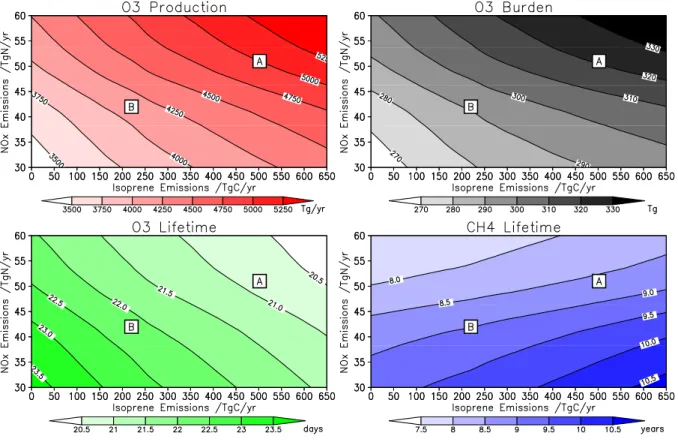
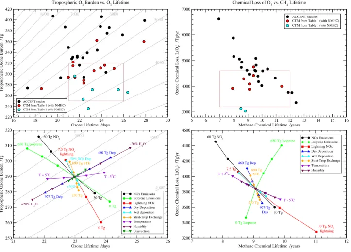
To explore the full sensitivity of the O3budget to emis-sions of NOx and isoprene, a series of 20 runs have been performed using isoprene emissions of 0, 220, 350, 500 and 650 TgC/yr and NOx emissions of 30, 42, 51 and 60 TgN/yr. Isoprene emissions were scaled linearly on the distribution of Guenther et al. (1995), while NOxemissions were varied non-linearly, with the 30 TgN/yr scenario repre-senting 1970 conditions and the 60 TgN/yr scenario scaled to IIASA current-legislation emissions for 2030 (Dentener et al., 2005). The variation in key budget terms is shown in Fig. 3. The gross production and burden of O3both increase steadily with increasing precursor emissions, consistent with the changes seen in the published budgets (see Fig. 1 and Ta-ble 1) and the O3lifetime is reduced as chemical destruction and deposition increase. The contrasting effects of NOxand

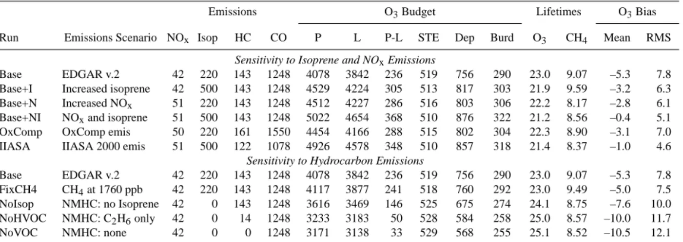
Table 3. Annual ozone budgets in the FRSGC/UCI CTM: sensitivity to precursor emissionsa.

Emissions O3Budget Lifetimes O3Bias

Run Emissions Scenario NOx Isop HC CO P L P-L STE Dep Burd O3 CH4 Mean RMS

Sensitivity to Isoprene and NOxEmissions

Base EDGAR v.2 42 220 143 1248 4078 3842 236 519 756 290 23.0 9.07 –5.3 7.8

Base+I Increased isoprene 42 500 143 1248 4529 4224 305 513 817 303 21.9 9.59 –3.2 6.3

Base+N Increased NOx 51 220 143 1248 4512 4227 286 516 803 306 22.2 8.17 –2.8 6.1

Base+NI NOxand isoprene 51 500 143 1248 5022 4654 368 510 876 322 21.2 8.56 –0.4 5.1

OxComp OxComp emis 50 220 161 1550 4454 4166 288 515 802 304 22.3 8.90 –3.1 7.0

IIASA IIASA 2000 emis 51 500 122 1078 4926 4578 348 510 857 318 21.4 8.37 –1.0 4.6

Sensitivity to Hydrocarbon Emissions

Base EDGAR v.2 42 220 143 1248 4078 3842 236 519 756 290 23.0 9.07 –5.3 7.8

FixCH4 CH4at 1760 ppb 42 220 143 1248 4117 3877 241 518 760 292 23.0 9.49 –5.0 7.5

NoIsop NMHC: no Isoprene 42 0 143 1248 3616 3469 146 525 675 274 24.1 8.75 –7.6 10.0

NoHVOC NMHC: C2H6only 42 0 14 1248 3233 3183 50 528 584 258 25.0 8.57 –10.0 11.7

NoVOC NMHC: none 42 0 0 1248 3171 3138 33 529 568 255 25.1 8.52 –10.5 12.1

a_{Emissions/budgets in Tg yr}−1_{(TgN yr}−1_{for NOx, TgC yr}−1_{for isoprene and NMHC); O}

3lifetime to chemical loss and deposition in

days; CH4lifetime to removal by tropospheric OH in years; biases in ppb.

isoprene on OH lead to a balance such that the CH4lifetime remains little affected by the combined emissions changes between the BASE and IIASA scenarios. However, the gra-dient of the slope is steep, and small changes in either NOx or isoprene separately can affect the lifetime substantially.

Note that the effects seen here are dependent on the com-plexity of the chemical scheme used in the model. The sim-plified scheme used here does not include isoprene nitrates, and more detailed studies treating their formation and depo-sition have found this to be a significant channel for removal of both isoprene intermediates and NOx(P¨oschl et al., 2000; von Kuhlmann et al., 2004). It is not clear how many previ-ous studies have included this pathway, but it has been shown to lead to stabilization of O3production with increasing iso-prene emissions (Wu et al., 2007). The differing complexity of chemical schemes may be an important source of differ-ences between model studies and merits a more detailed in-vestigation.

Table 3 also shows the sensitivity of the budget terms to the treatment of hydrocarbon emissions. Use of a globally-uniform field of CH4 instead of a transported CH4 tracer avoids the long spin-up times associated with CH4, but is shown to have very little effect on the O3 budget or life-time. The CH4lifetime is extended by about 5%, reflecting a higher atmospheric burden in the stratosphere when using a globally-uniform field. Complete removal of all hydrocar-bon emissions leads to a reduction in O3production of about 900 Tg/yr, half of which is due to isoprene, and a reduction in O3burden of about 35 Tg (12%) compared with the BASE scenario. These results are consistent with those of Houwel-ing et al. (1998) shown in Table 1.

4.2 Sensitivity to physical processes

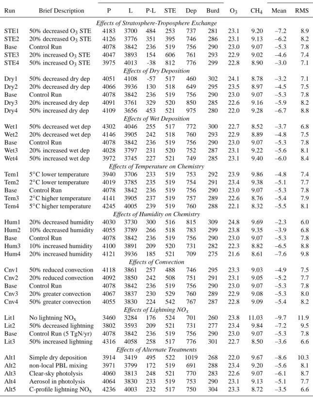
Meteorological and dynamical processes influence the pro-duction, mixing and removal of O3 both directly and indi-rectly. Humidity, temperature and UV flux govern chemical reaction rates, boundary layer turbulence and convection re-distribute O3 and its precursors, influencing O3 production and removal, and deposition processes remove O3and sol-uble precursors. Ozone chemistry in the upper troposphere is influenced by the magnitude and distribution of lightning-produced NOxemissions and by direct influx of O3from the stratosphere. Perturbation experiments are performed with the FRSGC/UCI CTM to explore the effect of these pro-cesses on O3, and the impacts on the key budget terms are shown in Table 4. For compatibility with the emissions stud-ies in Sect. 4.1, the same BASE control run was used.

The stratospheric influx of O3was increased by applying a consistent scaling of stratospheric Linoz chemistry. This leads to increased chemical removal and deposition in the troposphere, but also to decreased O3production, as noted by Wauben et al. (1998), due to faster removal of NOx. Of the additional O3 transported from the stratosphere, about 60% is destroyed chemically, 10% is deposited at the sur-face, and 30% displaces O3 that would have been formed in the troposphere, and is thus accounted for by decreased production. Quantifying the impact of STE on the tropo-spheric burden and lifetime of O3 is complicated by the choice of tropopause, however. Applying a thermal or dy-namical tropopause or using the same location as in the con-trol run leads to a large increase in the burden and an increase in lifetime associated with additional O3at high altitude. Ap-plying an O3 tracer tropopause, as here, leads to a much smaller increment in the burden as the tropospheric domain

Fig. 3. Isopleth plots showing the variations in O₃production, O₃ burden and the tropospheric lifetimes of O₃ and CH₄ for different

combinations of NOxand Isoprene emissions using the FRSGC/UCI CTM with 1996 meteorology at T21 resolution. The BASE run (“B”)

and IIASA run for the ACCENT studies (“A”) are indicated.

shrinks, and the O3lifetime shows a marginal decrease, see Table 4. Use of a tracer tropopause clearly damps the calcu-lated budget response to changes in STE. As removal of O3 by dry deposition changes only slowly along with the burden, the net impact of chemistry, P-L, is very sensitive to the STE flux used.

Dry deposition affects the O3budget directly by surface removal of O3and indirectly by removal of precursors such as NOxand PAN. Dry deposition velocities were altered for all species simultaneously in this sensitivity study. Increased O3deposition is balanced largely by decreased chemical loss due to lower O3, with a small increase in production caused by lower OH and hence an increased lifetime for NOx. De-creased chemical loss of O3is responsible for lower OH for-mation and hence for the increased CH4 lifetime. The net impact of chemistry is very sensitive to dry deposition as the net STE flux changes only marginally in response to changes in the tropospheric burden. Note the non-linear response of the dry deposition rate to the applied increases in deposi-tion velocity as the surface O3abundance falls. In contrast, wet deposition does not affect O3 directly but leads to the removal of soluble species such as HNO3and H2O2 which influence the availability of NOxand OH. Increasing removal

of these species by 50% causes both production and loss of O3to fall by about 2.5%, and the tropospheric burden drops proportionately. The small drop in net chemical production is balanced by reduced dry deposition, and the lifetime of O3 is little affected. However, the decrease in OH leads to a sig-nificant increase in the lifetime of CH4, and the OH response is 60–90% larger than for equivalent changes in the dry de-position rate. A non-linear response is also evident here, as a 50% reduction in wet deposition rates has twice the effect on the O3burden and removal as a 50% increase.

The effects of temperature and humidity on oxidant chem-istry are examined by applying small, globally uniform changes representative of the uncertainty in meteorological fields to the chemistry only. Increases in temperature affect chemical reaction kinetics and lead to significantly increased O3production and loss rates, but net production and other key budget terms are largely unaffected, and the tropospheric burden drops by less than 1% for a temperature rise of 5◦C. However, the faster chemistry leads to a higher abundance of OH, and the CH4lifetime is reduced by almost 10% for a 5◦C rise. This sensitivity of CH4oxidation to temperature provides a small negative feedback on climate warming, as noted by Fiore et al. (2006), and highlights temperature as a

Table 4. Annual ozone budgets in the FRSGC/UCI CTM: sensitivity to physical processesa.

O3Budget Lifetimes O3Bias

Run Brief Description P L P-L STE Dep Burd O3 CH4 Mean RMS

Effects of Stratosphere-Troposphere Exchange

STE1 50% decreased O3STE 4183 3700 484 253 737 281 23.1 9.20 –7.2 8.9

STE2 20% decreased O₃STE 4126 3776 351 395 746 286 23.1 9.13 –6.2 8.2

Base Control Run 4078 3842 236 519 756 290 23.0 9.07 –5.3 7.8

STE3 20% increased O3STE 4047 3893 154 606 761 293 22.9 9.02 –4.6 7.4

STE4 50% increased O3STE 3975 4013 -38 812 776 299 22.8 8.90 –3.0 7.1

Effects of Dry Deposition

Dry1 50% decreased dry dep 4051 4108 -57 517 460 302 24.1 8.78 –3.2 7.1

Dry2 20% decreased dry dep 4066 3936 130 518 649 295 23.5 8.97 –4.5 7.5

Base Control Run 4078 3842 236 519 756 290 23.0 9.07 –5.3 7.8

Dry3 20% increased dry dep 4091 3761 329 520 850 285 22.6 9.16 –5.9 8.2

Dry4 50% increased dry dep 4109 3656 453 521 975 280 22.0 9.28 –6.7 8.8

Effects of Wet Deposition

Wet1 50% decreased wet dep 4302 4046 255 517 772 300 22.7 8.52 –3.7 6.8

Wet2 20% decreased wet dep 4146 3905 242 518 760 293 22.9 8.89 –4.8 7.5

Base Control Run 4078 3842 236 519 756 290 23.0 9.07 –5.3 7.8

Wet3 20% increased wet dep 4028 3797 231 520 752 287 23.1 9.22 –5.6 8.1

Wet4 50% increased wet dep 3972 3745 227 521 749 285 23.1 9.40 –6.0 8.4

Effects of Temperature on Chemistry

Tem1 5◦C lower temperature 3940 3706 233 519 753 292 23.9 9.86 –4.8 7.4

Tem2 2◦C lower temperature 4019 3785 235 519 754 291 23.4 9.38 –5.1 7.7

Base Control Run 4078 3842 236 519 756 290 23.0 9.07 –5.3 7.8

Tem3 2◦C higher temperature 4141 3905 237 519 757 289 22.6 8.76 –5.4 7.9

Tem4 5◦C higher temperature 4245 4005 239 519 760 288 22.1 8.32 –5.5 8.1

Effects of Humidity on Chemistry

Hum1 20% decreased humidity 4030 3730 300 516 815 309 24.8 9.69 –2.3 6.0

Hum2 10% decreased humidity 4055 3789 266 518 783 299 23.8 9.35 –3.9 6.8

Base Control Run 4078 3842 236 519 756 290 23.0 9.07 –5.3 7.8

Hum3 10% increased humidity 4100 3891 209 520 731 282 22.3 8.82 –6.5 8.8

Hum4 20% increased humidity 4121 3936 185 521 709 275 21.6 8.61 –7.6 9.8

Effects of Convection

Cnv1 50% reduced convection 4118 3861 257 488 746 295 23.3 9.03 –4.9 7.5

Cnv2 20% reduced convection 4092 3850 242 508 751 291 23.1 9.05 –5.2 7.7

Base Control Run 4078 3842 236 519 756 290 23.0 9.07 –5.3 7.8

Cnv3 20% greater convection 4067 3837 230 529 760 289 22.9 9.08 –5.3 8.0

Cnv4 50% greater convection 4055 3830 224 542 767 287 22.8 9.09 –5.4 8.2

Effects of Lightning NOx

Lit1 No lightning NOx 3460 3284 176 524 701 260 23.8 11.03 –9.7 11.9

Lit2 50% decreased lightning 3802 3593 209 521 731 277 23.4 9.84 –7.2 9.5

Base Control Run (5 TgN/yr) 4078 3842 236 519 756 290 23.0 9.07 –5.3 7.8

Lit3 50% increased lightning 4316 4058 258 517 776 301 22.7 8.50 –3.6 6.6

Effects of Alternate Treatments

Alt1 Simple dry deposition 3914 3419 495 522 1019 268 22.0 9.67 –8.6 10.3

Alt2 non-local PBL mixing 3971 3799 172 519 691 288 23.4 9.20 –5.6 8.1

Alt3 Clear-sky photolysis 4060 3813 248 521 770 283 22.6 9.07 –6.1 8.7

Alt4 Aerosol in photolysis 4064 3830 233 519 753 290 23.1 9.13 –5.1 7.7

Alt5 C-profile lightning NOx 4236 4003 232 517 750 304 23.3 8.72 –3.5 6.6

a_{Budgets in Tg yr}−1_{; lifetimes in days for O}

significant source of uncertainty in model-derived CH4 life-times, as noted by Stevenson et al. (2000). Increased humid-ity leads to more efficient O3loss and greater OH production. Additional OH boosts O3production, but this only makes up about 45% of the additional O3loss, and net production falls. Surface deposition falls by about 6% with a 20% increase in humidity, balancing the increased chemical loss, and the O3 burden is reduced by 5%. The global O3 burden is much more sensitive to changes in humidity than in temperature, and the CH4lifetime is also strongly affected. Note that the uncertainty in the tropospheric water vapour burden in cur-rent climate models is about 10% (Stevenson et al., 2006), and this would introduce a 3% (9 Tg) variability in the O3 burden, a 3% (0.8 day) variability in O3 lifetime and a 3% (0.3 year) variability in CH4lifetime based on these sensitiv-ity studies.

Deep convection mixes O3-rich air from the upper tropo-sphere down towards the surface where the O3 lifetime is shorter and lifts freshly-emitted O3precursors into the upper troposphere where O3production may be greater. Previous studies with and without convective transport have disagreed on the relative importance of these pathways, with Lawrence et al. (2003) finding a 12% increase in O3 burden when in-cluding convection due to the dominant effect of increased production, and Doherty et al. (2005) finding a 14% decrease in burden as greater descent and destruction outweighed in-creased production. In the present study smaller changes in convection have been applied, and these were allowed to af-fect convective washout as well as lifting processes, unlike in the previous studies. Stronger convection leads to increased O3production in the upper troposphere but to decreased pro-duction in the lower troposphere, where precursors are re-moved by greater convective lifting and washout. There is an increase in the inferred influx from the stratosphere, re-flecting both convective steepening of the O3gradient near the tropopause and direct convective penetration above the monthly-mean tracer tropopause used here. Greater tropo-spheric overturning leads to higher surface O3 and greater deposition, and the tropospheric burden decreases. Compar-ison with the wet deposition sensitivity runs presented above suggests that this is partly due to increased washout, and that the effect of lifting alone is small. These results lie mid-way between those presented by Lawrence et al. (2003) and Doherty et al. (2005), and highlight the large uncertainty in modelled O3responses to convection. It is not clear if this uncertainty reflects differences in convection schemes, light-ning emissions or chemical complexity, as discussed in Do-herty et al. (2005), but the uncertainty is sufficiently large that this topic would be a valuable target for future model intercomparison studies.

The magnitude and distribution of lightning-produced NOxemissions are highly uncertain (e.g., Price et al., 1997) but are important for O3due to the longer lifetime of NOxin the upper troposphere and its greater efficiency for O3 pro-duction. This sensitivity is examined here by varying the

magnitude of lightning emissions from 0 to 7.5 TgN/yr in steps of 2.5 TgN/yr. Increased emissions cause a large in-crease in production and in tropospheric burden, as seen in previous studies (Labrador et al., 2005); about 10% of the additional O3 produced is removed by deposition, and the rest is destroyed by chemistry, contributing to a higher abun-dance of OH and to a reduced CH4 lifetime. The sensitiv-ity of the O3burden and the CH4lifetime are notably larger than for the other processes considered here. The range of lightning emissions used in the ACCENT model studies, 3– 8 TgN/yr, would account for a 10% difference in O3burden, a 0.7 day difference in O3lifetime and a 1.4 year difference in CH4lifetime between models. Note also that the study here uses vertically-uniform emission profiles for inter-cloud and cloud-to-ground lightning strokes based on Price and Rind (1992). Use of more realistic profiles based on observations (Pickering et al., 1998) (run Alt5) leads to a 25% greater in-crease in O3production and a 50% greater increase in burden for the same 5 TgN/yr emissions increase, as a greater pro-portion of the NOxemissions occur at high altitudes where the lifetimes of O3and NOxare longer.

Finally, a number of additional sensitivities related to model methodology have been examined, see Table 4. The dry deposition scheme of Isaksen et al. (1985) used in some studies (e.g., Berntsen et al., 1996; Wild and Prather, 2000; Zeng and Pyle, 2005) is a simpler alternative to the resistances-in-series scheme of Wesely (1989) used here. Application of this scheme with 1-m deposition velocities from Hough (1991) leads to 30% greater O3deposition, an additional 260 Tg/yr. Faster removal of NOxsuppresses pro-duction, but chemical destruction falls by a greater margin to compensate for the increased deposition. The tropospheric O3burden is almost 10% less than in the BASE run, and un-derestimation of the ozonesonde measurements suggest that the deposition rate with this scheme is too high. However, the lack of good observational constraints on deposition pre-vents this from being determined uniquely. The deposition rate is also reduced by application of a non-local boundary layer mixing scheme (Holtslag and Boville, 1993) in place of the simple hourly bulk-mixing used in the BASE run. Less efficient vertical mixing leads to stronger near-surface gradi-ents and reduced deposition of O3, but a smaller proportion of NOxescapes into the free troposphere, so chemical pro-duction is suppressed. The net effect of these changes on the global burden is small, less than 1%.

A major source of uncertainty not considered here is in the calculation of photolysis rates. A number of different meth-ods are currently used, ranging in complexity from tabulated rates based on climatological conditions to fully-interactive schemes accounting for absorption and scattering of aerosol and cloud particles calculated on-line. A simple test remov-ing all cloud cover in the interactive Fast-J scheme used here (Wild et al., 2000) indicates that the global budget of O3 is relatively insensitive to cloud cover. However, global O3 production at the surface is 15% higher without cloud cover,

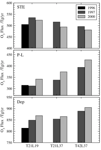
400 450 500 550 600 O 3 Flux /Tg/yr 1996 1997 2000 300 350 400 450 O 3 Flux /Tg/yr T21L19 T21L37 T42L37 750 800 850 900 950 O 3 Flux /Tg/yr STE P-L Dep

Fig. 4. Effects of meteorology and model resolution on the annual

flux of O3through stratosphere-troposphere exchange (STE), net

chemistry (P-L) and surface deposition (Dep).

balanced by lower production in the upper troposphere, and regional and seasonal differences can be much larger. The global O3burden change of 2.5% is comparable to the 3–5% changes found by Liu et al. (2006), but is clearly smaller than the 8–12% changes found by Tie et al. (2003), suggesting that the impacts may depend on details of the cloud scheme used. Inclusion of monthly-mean aerosol fields for the scat-tering code similarly lead to regional differences in O3 pro-duction, but the global impacts appear to be small.

4.3 Sensitivity to meteorology and resolution

Differences in meteorological data may affect the O3 bud-get through self-consistent variations in the physical pro-cesses considered in Sect. 4.2. Meteorological data from the ECMWF-IFS model for 1997 and 2000 are compared with the fields for 1996 used in this study, and the impact on the O3budget is shown in Table 5 and in Fig. 4. The CTM is run at T21L19 with each meteorology, and is additionally run at T21L37 and T42L37 to test the effects of doubled

verti-cal and horizontal resolution. The lower resolution fields are derived from the parent T42L37 data so that advective and convective mass fluxes are the same across the different reso-lutions. Precursor emissions are taken from IIASA for closer comparison with the ACCENT studies, and the same emis-sions are used for each year. For this sensitivity study only, total lightning NOxemissions are constrained to 6.5 TgN/yr and are distributed vertically following the profiles of Pick-ering et al. (1998); the geographical distribution of the emis-sions differs from year to year following the occurrence of deep convection events. Differences in O3burden and life-time between the different years are small, but differences in STE, deposition and chemistry reach 7–8%. The lifetime of CH4is 5% longer in 1997 than in 2000, suggesting that OH levels are significantly lower and reflecting shifts in humidity and convection during the 1997–1998 El Ni˜no period (Chan-dra et al., 1998; Sudo et al., 2001). The chemical production of O3 is lower in 1997, and influx from the stratosphere is greater. These results are in good qualitative agreement with those of Zeng and Pyle (2005) who examined the evolution of the O3budget between 1990 and 2001 with a global cli-mate model. The magnitude of this interannual variability in-dicates that model intercomparisons focussed on differences due to chemical or dynamical schemes should recommend use of the same meteorological fields.

Model O3budgets are sensitive to the horizontal and ver-tical resolution used, both through their effects on transport and mixing processes and through their impacts on O3 chem-istry from the spatial averaging of emissions (e.g., Chat-field and Delany, 1990). At the highest resolution used here, T42L37, there is a significant reduction in STE (8%, 40 Tg/yr) compared with T21L19 due to better resolution of the tropopause and there is an increase in surface depo-sition (5%, 40 Tg/yr). Increased net chemical production (25%, 80 Tg/yr) balances the budget, but there is a 2–4% drop in the O3 burden. The magnitude of these effects is highly consistent for 1997 and 2000 meteorology, and con-firms the results of previous studies (von Kuhlmann et al., 2003; Wild and Prather, 2006). It is worth noting that some studies have found greater STE at higher horizontal reso-lution (Kentarchos et al., 2001; van Noije et al., 2004), al-though this may be strongly influenced by excessive vertical motions in the lower stratosphere associated with the assimi-lation methods used during generation of meteorological re-analyses (Douglass et al., 1996; van Noije et al., 2006). The changes due to resolution seen here are similar in magnitude to those with different meteorological fields, but are system-atic in nature. Increased vertical resolution has relatively lit-tle effect on gross chemical production or surface deposition, but accounts for at least half of the decrease in STE and for about one third of the increase in net production. Increased horizontal resolution dominates the changes in deposition and gross chemical production due to better localisation of boundary layer O3, its production and convection, and bet-ter resolution of the tropopause region leads to an additional

Table 5. Annual ozone budgets in the FRSGC/UCI CTM: sensitivity to meteorology and resolutiona.

Meteorological Data O₃Budget Lifetimes O₃Bias

Run Description Resolution Year P L P-L STE Dep Burd O3 CH4 Mean RMS

Met96 IFS 1996 data T21 L19 1996 5247 4932 315 505 814 342 21.7 8.38 2.1 5.0

Met97 IFS 1997 data T21 L19 1997 4975 4663 312 535 849 336 22.2 8.79 0.9 5.9

Met97L – 37 levels T21 L37 1997 5103 4766 338 516 854 340 22.1 8.54 2.3 6.0

Met97R – T42 resolution T42 L37 1997 4982 4588 394 496 889 331 22.0 8.89 1.5 5.3

Met00 IFS 2000 data T21 L19 2000 5314 4972 342 524 869 345 21.5 8.02 2.4 5.6

Met00L – 37 levels T21 L37 2000 5310 4935 374 494 865 341 21.5 8.10 2.1 5.3

Met00R – T42 resolution T42 L37 2000 5160 4734 427 481 905 331 21.4 8.45 1.7 4.3

a_{Budgets in Tg yr}−1_{; lifetimes in days for O3and years for CH4; biases in ppb.}

reduction in STE. Although the mean tropospheric lifetime of O3is only marginally affected by increased resolution, the chemical lifetime of CH4 is substantially increased, by as much as 5% for the 2000 case, reflecting lower OH and O3 production at higher resolution.

4.4 Examining inter-model variability

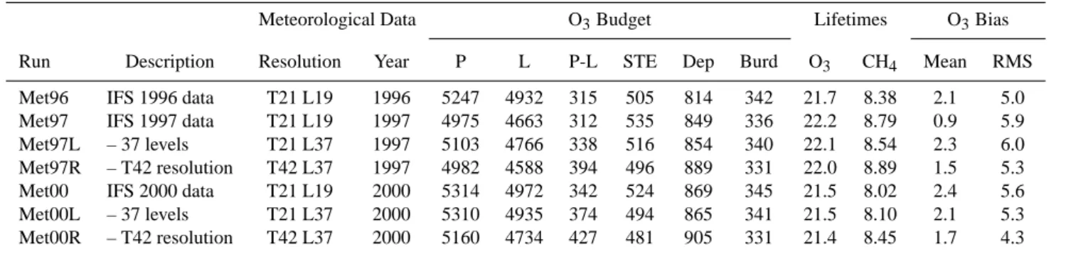
To what extent do the sensitivities examined here account for the variability in published model budgets seen in Ta-ble 1? The results of these sensitivity studies and of earlier published studies are shown in Fig. 5. The variability is ex-amined in two different parameter spaces which summarize the fate of O3and the abundance of OH, following Steven-son et al. (2006). Results from published model studies and from individual models from the ACCENT model intercom-parison are shown in Figs. 5a and b, and results from the sen-sitivity studies over part of these parameter spaces are shown in Figs. 5c and d. The sensitivities examined here do not re-flect the same level of uncertainty in the different variables, but are intended to be loosely comparable so that the relative importance of different processes is evident.

Differences in the abundance and fate of O3are revealed by the relationship between the tropospheric burden and the lifetime of O3 to chemical removal and deposition and are shown in Fig. 5a. Inclusion of hydrocarbon chemistry and in-creased surface emissions lead to higher burdens and shorter lifetimes, but cannot account for the large spread in bur-den (274–407 Tg), lifetime (17–28 years) and removal rate (4500–7600 Tg/yr) seen in the ACCENT studies where emis-sions varied little. Figure 5c suggests that differences in hu-midity and in surface deposition may make important contri-butions to this variation, as they affect the O3 burden and lifetime without changing gross tropospheric removal sig-nificantly. A 10% variation in humidity and a 200 Tg/yr variation in dry deposition, as seen in the ACCENT stud-ies (Stevenson et al., 2006), could each account for 9 Tg in O3burden and 1 day in O3lifetime. Variations in

tempera-ture and convection have a similar but smaller effect. Wet deposition and STE lead to changes in the gross removal of O3, but the scatter in this dimension is strongly influ-enced by emissions. Lightning NOx emissions varied be-tween 3 and 8 Tg/yr for the ACCENT models and may ac-count for 30 Tg in O3burden and 500 Tg/yr in O3removal. Isoprene emissions varied between 220 and 630 TgC/yr, and may thus account for 20 Tg in O3burden and 650 Tg/yr in O3 removal. Differences in meteorological data reflecting inter-annual variability between the three years studied here intro-duce less variability, about 5 Tg in O3burden and 0.5 days in O3lifetime, although increased resolution may lead to a 5– 15 Tg reduction in burden. However, the sensitivity studies performed here clearly do not account for the full variability in O3budgets seen in the ACCENT runs, and it is likely that differences in chemical mechanisms, in model dynamics, and in the reanalysis methods used to generate the meteorological data also make large contributions to this variability.

The relationship between the chemical loss of O3, govern-ing the source of OH, and the lifetime of CH4, controlled by OH, is shown in Fig. 5b. The variability in this relationship is more restricted, and most points lie close to a single line, as processes that increase O3production and loss are associated with a higher level of OH and hence with a shorter CH4 life-time. Surface emissions of isoprene have a significantly dif-ferent effect, however, as greater OH formation from higher O3production and loss is outweighed by the direct removal of OH that initiates hydrocarbon oxidation, and thus CH4 lifetime increases with higher isoprene emissions as other studies have noted (von Kuhlmann et al., 2004). Ozone loss and CH4lifetime are systematically lower in model studies omitting higher hydrocarbons. The mean chemical lifetime of CH4from the ACCENT studies is 9.8 years, close to the 9.6 years recommended by Prather and Ehhalt (2001), but the variability is large, 6.9–15.2 years. This variability implies a large uncertainty in CH4emissions, as the global CH4 bur-den is relatively well constrained. The variation in lightning

16 18 20 22 24 26 28 30 Ozone Lifetime /days

220 240 260 280 300 320 340 360 380 400 420

Tropospheric Ozone Burden /Tg

ACCENT studies CTM from Table 1 (with NMHC) CTM from Table 1 (w/o NMHC)

Tropospheric O₃ Burden vs. O₃ Lifetime

5000 4000 6000 7000 8000 5 6 7 8 9 10 11 12 13 14 15 16

Methane Chemical Lifetime /years 3000

4000 5000 6000 7000

Ozone Chemical Loss, L(O

3

) /Tg/yr

ACCENT Studies CTM from Table 1 (with NMHC) CTM from Table 1 (w/o NMHC)

Chemical Loss of O₃ vs. CH₄ Lifetime

21 22 23 24 25 26

Ozone Lifetime /days 250 260 270 280 290 300 310 320

Tropospheric Ozone Burden /Tg

NOx Emissions Isoprene Emissions Lightning NOx Dry Deposition Wet deposition Strat-Trop Exchange Temperature Humidity Convection 5000 4000 4500 60 Tg NO_x 650 Tg Isoprene -20% H2O 800 Tg STE T - 5oC 7.5 Tg NO_x lightning 460 Tg Dep 975 Tg Dep +20% H₂O 250 Tg T + 5oC 30 Tg 0 Tg 0 Tg -50% Wet Dep +50% 7 8 9 10 11 12

Methane Chemical Lifetime /years 3200 3400 3600 3800 4000 4200 4400 4600

Ozone Chemical Loss, L(O

3 ) /Tg/yr NOx Emissions Isoprene Emissions Lightning NOx Dry Deposition Wet Deposition Strat-Trop Exchange Temperature Humidity 60 Tg NOx 650 Tg Isoprene T + 5oC 460 Tg Dep 0 Tg NOx lightning 0 Tg Isoprene 30 Tg T - 5oC 7.5 Tg 975 Tg Dep 800 Tg STE 250 Tg

Fig. 5. The relationship between the tropospheric burden of O3and its lifetime to chemical removal and deposition (left panels, a and c) and

between the chemical removal of O3and the chemical lifetime of CH4(right panels, b and d). The upper panels (a and b) show results from

published studies summarized in Table 1 and the lower panels (c and d) show the results of sensitivity studies listed in Table 3. Tropospheric

O3removal rates versus chemistry and deposition are shown as diagonal lines in the left panels (labelled in Tg/yr). For ease of comparison

the domain of the sensitivity studies shown in the lower panels c and d is highlighted in the upper panels with a box.

NOxemissions may account for almost 1.5 years in the CH4 lifetime, but differences in temperature, humidity, wet and dry deposition, and STE also contribute significantly to this variability. The abundance of OH is very sensitive to the chemistry and photolysis schemes used, and the effects of these have not been examined in this study. However, deter-mination of the climate impacts of CH4and other trace gases depends on a reliable quantification of chemical removal by OH, and the large variability seen in the ACCENT studies suggests that further work is needed to reduce the uncertainty in current models.

To estimate the contribution of the processes examined here to the variability in the budget terms from the ACCENT intercomparison, the O3 budget terms for each model are standardized by applying corrections based on the sensitiv-ities derived with the FRSGC/UCI CTM, see Table 6. A sen-sitivity factor for the change in each of these budget terms

Table 6. Budget terms from the ACCENT model intercomparison

corrected for different surface and lightning emissions, dry deposi-tion and STE fluxes.

O3Prod O3Loss CH4Lifetime

(Tg/yr) (Tg/yr) (years)

ACCENT study 5110±606 4668±727 9.79±1.74

Standardization: All 5110±506 4668±518 9.71±1.33

Standardization of Separate Processes

NOxemissions only 5110±596 4668±721 9.78±1.72

Isoprene emissions only 5110±539 4668±667 9.78±1.73 Lightning NOxonly 5110±563 4668±656 9.72±1.42

Dry Deposition only 5110±608 4668±664 9.78±1.69

with respect to STE, dry deposition, lightning and surface emissions is derived from Table 4, and a correction is then applied for each model by scaling the sensitivity factor by the deviation from the ACCENT ensemble mean. As an ex-ample, the sensitivity factor for O3production from lightning NOxemissions is 150 Tg/TgN based on run Alt5 in Table 4, and the ensemble mean lightning emission is 5.7 TgN/yr, so the correction for gross O3production for a model with 5.0 TgN/yr lightning NOxis +105 Tg/yr. Note that this sim-ple approach assumes a linear response and therefore the en-semble mean production and loss terms remain unaltered. However, this standardization leads to a reduction in the 1σ variability of 100 Tg/yr for production and 200 Tg/yr for loss when applied to all budget terms considered here, and the difference between the outlying models is reduced by more than 35%. The largest contributions to this reduced vari-ability in production come from standardizing the isoprene emissions and lightning NOx, while for chemical loss there is also a large impact from standardizing deposition. There is a small decrease in the mean CH4lifetime as corrections are applied to CH4loss rates, but the 1σ variability in the CH4 lifetime is reduced by about 25%, from 1.7 to 1.3 years, and the difference between the outlying models is also reduced by 25%. Lightning NOxemissions make the largest contri-bution to this reduced variability. Although this standardiza-tion is approximate, it demonstrates that the biases imposed by the treatment of these processes are systematic, and that the differences between models would be reduced in more tightly constrained studies.

5 Conclusions

This study has examined how the tropospheric O3budget cal-culated in global CTMs has evolved over the past decade and has explored the sensitivity of the key budget terms to vari-ability in precursor emissions, physical processes and mete-orology. Large differences apparent in early CTM studies reflect overestimation of stratosphere-troposphere exchange and omission of hydrocarbon chemistry. The increases in O3production and tropospheric burden in more recent stud-ies are principally due to use of higher surface emissions of NOxand isoprene. The higher NOxemissions largely reflect a better understanding of sources and emission factors, while higher isoprene emissions suggest greater confidence in the large emission estimates within the modelling community. Increases in these emissions alone lead to an increase in O3 production of 1100 Tg/yr in the FRSGC/UCI CTM, account-ing for about 66% of the increase in production seen between the IPCC-TAR and ACCENT studies. Recent analysis by Wu et al. (2007) has shown similar results. Comparison with ozonesonde measurements suggests that precursor emissions used in earlier studies were too low, and that O3distributions are reproduced better with recent IIASA emissions data.

The burden of O3 in the troposphere in CTMs has in-creased from around 300 Tg to around 340 Tg following the increase in precursor emissions, but is strongly influ-enced by the tropopause definition used. Comparison of three O3climatologies with seven different tropopause defi-nitions suggests that as much as ±15% of the variability in the burden may be due to the choice of tropopause. Recent model assessments have recommended use of an O3tracer tropopause of 150 ppb (Prather and Ehhalt, 2001), and this provides a robust definition consistent with that of a dynam-ical tropopause based on PV, giving a tropospheric burden of 335±10 Tg with the monthly-mean measurement clima-tologies used here. The mean burden from the ACCENT model intercomparison is 344 Tg, close to this value, but the 1σ variability remains large, 39 Tg, even with consistent use of the 150 ppb O3 tracer tropopause, highlighting substan-tial differences in O3distribution between the models. Fur-ther exploration of the sensitivity of the mean burden and the cross-tropopause flux to the choice of upper boundary for O3 and to the reanalysis method used in generating the meteo-rology would be valuable.

Sensitivity studies have been performed to examine how differences in key model processes might account for the difference in O3 budget terms seen in the relatively well-constrained ACCENT model intercomparison. The magni-tude and vertical distribution of lightning NOx emissions is shown to be a major source of uncertainty, and the 3– 8 TgN/yr range in the ACCENT study may account for a 10% difference in tropospheric ozone burden (about 30 Tg) and a 1.4 year difference in CH4lifetime. This accounts for about 10% of the variability in the ACCENT O3budgets and al-most 20% of the variability in the CH4 lifetime. Processes affecting the O3 distribution, such as dry deposition, STE, and convection, and those affecting chemical production and loss, such as temperature, humidity, photolysis and wet re-moval of precursors, also have an important role and may account for much of the year-to-year variability in the bud-gets of O3and CH4. The uncertainty in these processes is not well characterised, but dry deposition, STE and surface and lightning emissions account for about 25% of the model vari-ability in the ACCENT intercomparison. The large spread in CH4lifetime suggests that the climate response of changes in O3precursors in current models may differ substantially. Tighter constraints on lightning NOx emissions and meteo-rological fields would allow future model intercomparisons to focus more closely on the impacts of different chemistry schemes and different parameterizations of convection and mixing which are difficult to discern from recent studies.

Further development of CTMs with greater chemical de-tail, better treatment of scavenging and aerosol processes and finer resolution of small-scale processes is expected to lead to refinement of the O3 budget terms explored here. As improved parameterizations of the key processes be-come available, widely-differing models should start to con-verge on the same budget terms, with differences driven