Global ozone and air quality: a multi-model assessment of risks to human health and crops

(1)

HAL Id: hal-00328266

https://hal.archives-ouvertes.fr/hal-00328266

Preprint submitted on 10 Oct 2008

HAL is a multi-disciplinary open access

archive for the deposit and dissemination of sci-entific research documents, whether they are pub-lished or not. The documents may come from teaching and research institutions in France or abroad, or from public or private research centers.

L’archive ouverte pluridisciplinaire HAL, est destinée au dépôt et à la diffusion de documents scientifiques de niveau recherche, publiés ou non, émanant des établissements d’enseignement et de recherche français ou étrangers, des laboratoires publics ou privés.

Global ozone and air quality: a multi-model assessment

of risks to human health and crops

K. Ellingsen, M. Gauss, R. van Dingenen, F. J. Dentener, L. Emberson, A. M.

Fiore, M. G. Schultz, D. S. Stevenson, M. R. Ashmore, C. S. Atherton, et al.

To cite this version:

K. Ellingsen, M. Gauss, R. van Dingenen, F. J. Dentener, L. Emberson, et al.. Global ozone and air quality: a multi-model assessment of risks to human health and crops. 2008. �hal-00328266�

(2)

ACPD

8, 2163–2223, 2008 Multi-model assessment of ozone pollution indices K. Ellingsen et al. Title Page Abstract Introduction Conclusions References Tables Figures ◭ ◮ ◭ ◮ Back Close

Full Screen / Esc

Printer-friendly Version Interactive Discussion

EGU

Atmos. Chem. Phys. Discuss., 8, 2163–2223, 2008 www.atmos-chem-phys-discuss.net/8/2163/2008/ © Author(s) 2008. This work is licensed

under a Creative Commons License.

Atmospheric Chemistry and Physics Discussions

Global ozone and air quality: a

multi-model assessment of risks to

human health and crops

K. Ellingsen1, M. Gauss1, R. Van Dingenen2, F. J. Dentener2, L. Emberson3, A. M. Fiore4, M. G. Schultz5, D. S. Stevenson6, M. R. Ashmore3, C. S. Atherton7, D. J. Bergmann7, I. Bey8, T. Butler9, J. Drevet8, H. Eskes10, D. A. Hauglustaine11, I. S. A. Isaksen1, L. W. Horowitz4, M. Krol2,*, J. F. Lamarque12, M. G. Lawrence9, T. van Noije10, J. Pyle13, S. Rast5, J. Rodriguez14, N. Savage13,**, S. Strahan14, K. Sudo15, S. Szopa11, and O. Wild15,***

1

University of Oslo, Department of Geosciences, Oslo, Norway 2

Joint Research Centre, Institute for Environment and Sustainability, Ispra, Italy 3

Stockholm Environment Institute, University of York, Heslington, UK 4

NOAA GFDL, Princeton, NJ, USA 5

Max Planck Institute for Meteorology, Hamburg, Germany 6

University of Edinburgh, School of Geosciences, Edinburgh, UK 7

Lawrence Livermore National Laboratory, Atmospheric Science Division, Livermore, USA 8

Ecole Polytechnique F ´ed ´erale de Lausanne (EPFL), Switzerland 9

Max Planck Institute for Chemistry, Mainz, Germany 10

Royal Netherlands Meteorological Institute (KNMI), De Bilt, The Netherlands 11

(3)

ACPD

Full Screen / Esc

EGU 12

National Center of Atmospheric Research, Atmospheric Chemistry Div., Boulder, CO, USA 13

University of Cambridge, Centre of Atmospheric Science, UK 14

Goddard Earth Science & Technology Center (GEST), Maryland, Washington, DC, USA 15

Frontier Research Center for Global Change, JAMSTEC, Yokohama, Japan ∗

now at: Wageningen University and Research Centre, Wageningen, the Netherlands ∗∗

now at: Met Office, Exeter, UK ∗∗∗

now at: Dept. of Environmental Science, University of Lancaster, Lancaster, UK Received: 22 November 2007 – Accepted: 20 December 2007 – Published: Correspondence to: M. Gauss (michael.gauss@geo.uio.no)

(4)

ACPD

Full Screen / Esc

EGU

Abstract

Within ACCENT, a European Network of Excellence, eighteen atmospheric models from the U.S., Europe, and Japan calculated present (2000) and future (2030) concen-trations of ozone at the Earth’s surface with hourly temporal resolution. Comparison of model results with surface ozone measurements in 14 world regions indicates that 5

levels and seasonality of surface ozone in North America and Europe are character-ized well by global models, with annual average biases typically within 5–10 nmol/mol. However, comparison with rather sparse observations over some regions suggest that most models overestimate annual ozone by 15–20 nmol/mol in some locations. Two scenarios from the International Institute for Applied Systems Analysis (IIASA) and 10

one from the Intergovernmental Panel on Climate Change Special Report on Emis-sions Scenarios (IPCC SRES) have been implemented in the models. This study fo-cuses on changes in near-surface ozone and their effects on human health and veg-etation. Different indices and air quality standards are used to characterise air quality. We show that often the calculated changes in the different indices are closely inter-15

related. Indices using lower thresholds are more consistent between the models, and are recommended for global model analysis. Our analysis indicates that currently about two-thirds of the regions considered do not meet health air quality standards, whereas only 2–4 regions remain below the threshold. Calculated air quality exceedances show moderate deterioration by 2030 if current emissions legislation is followed and slight 20

improvements if current emissions reduction technology is used optimally. For the “business as usual” scenario severe air quality problems are predicted. We show that model simulations of air quality indices are particularly sensitive to how well ozone is represented, and improved accuracy is needed for future projections. Additional mea-surements are needed to allow a more quantitative assessment of the risks to human 25

(5)

ACPD

Full Screen / Esc

EGU

1 Introduction

Elevated ground level ozone is harmful to human health, crops and natural ecosys-tems. WHO (2003) reported that exposure to high ozone levels is linked to respiratory problems, such as asthma and inflammation of lung cells. Ozone may also aggra-vate chronic illnesses such as emphysema and bronchitis and weaken the immune 5

system. Eventually, ozone may cause permanent lung damage. Enhanced ozone reduces agricultural and commercial forest yields, and alters plant vulnerability to dis-ease, pests, insects, other pollutants and harsh weather (USEPA, 1999; Aunan et al., 2000; Mauzerall and Wang, 2001; Emberson et al., 2003; Wang and Mauzerall, 2004). Model studies indicate that much of the world’s population and food production ar-10

eas are currently exposed to damagingly high levels of ozone (West and Fiore, 2005). This situation could dramatically worsen over the coming century (Prather et al., 2003). In particular, due to Asia’s rapid economic growth with associated consequences for increased environmental pollution, hemispheric transport of pollution, and rising back-ground ozone levels, new areas are likely to be exposed to ozone pollution. Recent 15

epidemiological studies have revealed damage to human health at typical present-day Northern Hemisphere background levels (i.e. 30–40 nmol/mol) (WHO, 2003). Despite these major concerns, there has been little research focused on quantifying the risks of future exposure of the global biosphere to enhanced ozone levels (Ashmore, 2005) or on assessing potential health impacts on the global scale.

20

Ozone is formed when carbon monoxide (CO) and volatile organic compounds (VOC) are photo-oxidized in the presence of nitrogen oxides and sunlight, with ozone production occurring further downwind in the case of very high NOx emissions. El-evated surface ozone levels are therefore closely linked to emissions of these com-pounds from anthropogenic activity, including biomass burning. The atmospheric life-25

time of tropospheric ozone is long enough (1–2 weeks in summer to 1–2 months in win-ter) to be transported from a polluted region in one continent to another (e.g. Berntsen et al., 1999; Wild and Akimoto, 2001; Bey et al., 2001; Li et al., 2002; Auvray and

(6)

ACPD

Full Screen / Esc

EGU

Bey, 2005). Long-range transport can elevate the background level of ozone and add to locally or regionally produced ozone, sometimes leading to persistent exceedance of critical levels and air quality standards (e.g. Fiore et al., 2003). Regional efforts to control ozone increases through emission reductions of ozone precursors could be counteracted by unregulated growth in other regions and affect background concentra-5

tions on a global scale (e.g. Derwent et al., 2004).

The number of peak-level ozone episodes is currently stable or decreasing in Europe and the U.S. (USEPA, 2005; EMEP, 2005a; Jonson et al., 2006). However, in 2003, a year of unusually high temperature conditions in western and central Europe during summer, the EU threshold for informing the public (90 nmol/mol) was exceeded in 17 of 10

the 27 reporting countries (EMEP, 2005a). France, Spain and Italy regularly reported hourly peak concentrations in excess of 120 nmol/mol, levels which can cause serious health problems and damage to plants. The critical level for agricultural crops is ex-ceeded regularly at most EMEP stations in central Europe, as is the critical level for forests in larger parts of central and eastern Europe (EMEP, 2005b). There is evidence 15

that Northern Hemispheric background ozone levels increased by almost a factor of two (about 20 nmol/mol) since the 1950’s (Staehelin et al., 1994), and there are indi-cations that this increase is continuing, albeit at a slower rate (Simmonds et al., 2004). These trends are attributed to increases in global emissions of ozone precursors, in recent years mainly related to the rapid development in Asia (Akimoto, 2003). Future 20

surface ozone levels will mainly be determined by the development of emission con-trols of ozone precursors. The implications of the IPCC SRES scenarios (Nakicenovic et al., 2000) on future surface ozone levels were discussed by Prather et al. (2003) indicating that surface ozone in the Northern Hemisphere could increase by about 5 nmol/mol by 2030 (the range across all the SRES scenarios was 2–7 nmol/mol) and, 25

under the most pessimistic scenarios, by over 20 nmol/mol in 2100. Changes in cli-mate and atmospheric composition are mediated by eco-systems, which themselves respond to changes in climate. Climate change (i.e. changes in atmospheric dynamics, water vapor, temperature) can alter tropospheric formation, distribution and deposition

(7)

ACPD

Full Screen / Esc

EGU

of ozone (Sudo et al., 2003; Zeng and Pyle, 2003; Hauglustaine et al., 2005; Steven-son et al., 2005). Emission-climate feedbacks may result in changed emissions, such as increased biogenic VOC emissions in a warming atmosphere, and changes to the distribution and magnitude of lightning NOx emissions.

This study is part of a wider global model intercomparison called “ACCENT Photo-5

comp” coordinated under Integrated Activity 3 of ACCENT (“Atmospheric Composition Change: the European NeTwork of excellence”). ACCENT Photocomp (Experiment 2) focused on the global atmospheric environment between 2000 and 2030 using 26 state-of-the-art global atmospheric chemistry models and three emission scenarios. The present study uses a subset of 18 of these models that provided hourly sur-10

face ozone values. Several features of this intercomparison and further applications of model output have been published previously. An overview of model results was given by Dentener et al. (2006a). Stevenson et al. (2006) studied tropospheric ozone changes and the associated climate forcings and showed that the model ensemble mean for O3 generally agreed well with ozone observations in the free troposphere, 15

with the mean values nearly always within a standard deviation of each other. Van Noije et al. (2006) compared modeled NO₂with three GOME retrieved NO₂ columns: the range encompassed by models was often as large as that from the three retrievals. Dentener et al. (2006b) assessed present and future reactive sulphur and nitrogen de-position, Szopa et al. (2006, 2007) used the modeled ozone fields for a regional model 20

study of future air quality in Europe, and Shindell et al. (2006) showed that modeled CO was systematically underestimated by all models when comparing with surface mea-surements and satellite retrievals. It has to be noted, however, that the models used specified emissions and that the underestimation primarily reflects uncertainties in the emissions.

25

This publication focuses on the ability of global models to represent current surface ozone spatial and temporal distributions, the exceedance of ozone air quality indices and their possible development towards 2030. We collected the hourly surface ozone concentrations from a large number of models. This exercise was the first time that

(8)

ACPD

Full Screen / Esc

EGU

hourly ozone from global models has been intercompared and used to evaluate global distributions of various ozone health- and vegetation-relevant air quality indices, based on the accumulation of hourly averaged concentrations above a given threshold (van Loon et al., 2007).

In the following section, we describe the models and the experimental setup. In 5

Sect. 3, we discuss a wide range of currently used air quality standards currently used for vegetation (AOT40, SUM06, and W126) and human health [European and Amer-ican standards, as well as the WHO recommended SOMO35] in the context of the ability of global models to represent them. In Sect. 4 results from the model calcula-tions are given. In Sects. 4.1 and 4.2 annual mean surface ozone levels are discussed 10

for all scenarios, and surface ozone levels for 2000 are compared to observations. We have compared model ensemble results for the 18 participating models, rather than individual model results, since in a previous study we showed that ensemble results were representative of the participating models, and that leaving out possible outliers had little effect on the ensemble results (Stevenson et al., 2006). In Sect. 5, the re-15

sults from the air quality standard studies are presented. We finish with a summary, conclusions, and an outlook.

2 Experimental setup

The key features of the 18 global atmospheric chemistry models that participated in this study are described in Table 1. Twelve of these models are chemistry-transport models 20

(CTMs) driven by meteorological analyses. Most models used analyses from ECMWF (European Centre for Medium-range Weather Forecasts). Six CTMs are driven by global circulation models (GCMs). The horizontal resolution ranges from 4◦×5◦ to 1.8◦×1.8◦, with one model using a two-way nested grid of 1◦×1◦ over Europe, North America and Asia. Models had between 19 and 60 vertical levels, and all extended 25

well into the stratosphere (see Stevenson et al., 2006, Table A1).

(9)

ACPD

Full Screen / Esc

EGU

of free tropospheric ozone to ozone soundings by Stevenson et al. (2006) showed that the model ensemble mean agreed well with the observations, with the mean values nearly always within a standard deviation of each other.

Five different simulations were performed (Table 2). Table 3 gives a summary of the simulations performed by the individual models, biogenic C5H8and lightning NOx 5

emissions used, and the height of the surface layer. S1 is the year 2000 base case simulation, whereas simulations S2, S3, and S4 used the same meteorology as S1 and three different 2030 emission scenarios. The CTMs used meteorological data from year 2000, the GCMs performed up to 9 year simulations with meteorological data for the 1990s. The GCMs provided data for all years, the indices being calculated for 10

each year separately and then averaged. Simulation S5 was performed by GCM-CTM models only, using the emission case of S2 and meteorology for the 2020s. All GCMs were configured as atmosphere-only models with prescribed sea-surface temperature (SSTs) and sea-ice distributions. Most GCMs used SSTs and sea-ice from a simulation of HadCM3 (Hadley Centre Coupled Model, version 3, Johns et al., 2003) forced by 15

the IS92a scenario (Leggett et al., 1992) for the 2030 climate. Some GCMs used their own climate simulations. Spin-up lengths of at least 3 months were applied for all experiments.

Gridded anthropogenic emissions on 1◦×1◦of NOx, CO, NMHC, SO2and NH3were specified. In order to reduce the spin-up time, global CH₄ mixing ratios were pre-20

scribed across the model domain (Table 4). The choice of CH4 values were based on two earlier studies (Dentener et al., 2005; Stevenson et al., 2005), together with IPCC recommendations for SRES A2 [IPCC, 2001, their Table II.2.2]. Emissions for the ref-erence year 2000 and the future scenarios “Current Legislation” (CLE) and “Maximum Feasible Reduction” (MFR) were based on recent inventories developed by the Inter-25

national Institute for Applied Systems Analysis (IIASA). The CLE scenario was based on legislation in place in the year 2001. We note here that recent emission legislation in India, adopting the EURO 3 standard for 4-wheel vehicles, could substantially reduce traffic emissions after 2010, but was not in place in time for this study. The global totals

(10)

ACPD

Full Screen / Esc

EGU

of the future scenarios were distributed spatially according to EDGAR3.2 (Olivier et al., 2001) as described in (Dentener et al., 2005). To evaluate a high-emission case we also used the IPCC SRES A2 (A2) scenario (Nakicenovic et al., 2000). Monthly vary-ing biomass burnvary-ing 1◦×1◦gridded distributions were specified from GFED1.0 (van der Werf et al., 2003), scaling NOxand VOC emissions to those of CO. The values are av-5

erages for the period 1997–2002 and were used for all future scenarios as we felt that any other assumption would be highly speculative. Following AEROCOM (Dentener et al., 2006c) ecosystem dependent height distributions for biomass burning (bound-aries at 0, 0.1, 0.5, 1.0, 2.0, 3.0 and 4.0 km) and industrial emissions (height range 100–300 m) were recommended. However, some models added emissions to the low-10

est model layer only, whereas GMI/CCM3, GMI/DAO, GMI/GISS, IASB, TM4, TM5 and UIO CTM2 used the recommendations for industrial emissions. These models as well as MOZ2-GFDL, LLNL-IMPACT and MOZECH also used the recommended height profile for biomass burning. The global totals of anthropogenic emissions (including biomass burning) for both the reference year and the future scenarios are reported in 15

Table 4.

In addition, aircraft NO_x emission totals of 0.8 Tg N/year for the year 2000 and 1.7 Tg N/year (all 2030 cases) and ANCAT or NASA [IPCC, 1999] distributions were recommended. Recommendations given on natural emissions are reported in Ta-ble 5. Lightning and soil NO_x emissions were requested to be approximately 5 and 20

7 Tg N/year respectively. Modelers used values in the range of 3.7–7.0 Tg N/year for lightning and 5.5–8.0 Tg N/year for soil emissions. A total annual emission of 512 Tg C/year isoprene (IPCC, 1999) was recommended; values in the range of 220– 631 Tg C/year were used. The actual isoprene and lightning NOx emissions used by each model are listed in Table 3.

25

A distribution of NMHC among individual species was recommended according to the specification given by (Prather et al., 2001, their Table 4.7). Species not included in the model were recommended to be either ignored or lumped into higher species.

(11)

ACPD

Full Screen / Esc

EGU

respective surface layers. The thicknesses of these surface layers vary from model to model and are listed in Table 3. Using these results for comparison with measurements and for calculating global air quality indices is not straightforward. The best reference level for comparing model results with ozone measurements and for calculating the exceedance of air quality indices would be at canopy height (typically 1–20 m, 1 m for 5

crops, 20 m for forests) or at the height of human exposure (typically 2 m). However, models report surface ozone averaged over the lowest model layer, which is usually well above the canopy. Since there can be significant vertical gradients due to dry deposition (ozone increasing with height), particularly under stable conditions, models most likely overestimate the air quality indices. Also, we should realize that global scale 10

models as used in this study can not resolve small scale (<100 km horizontal extent) peak episodes and are thus best suited to study the impact of background pollution levels. Where necessary we will indicate this important limitation in discussing the results of our study.

In Sect. 4 we focus on results calculated from the ensemble of individual models. Use 15

of an ensemble should improve the robustness of model results as individual model errors, except systematic biases from emissions, are likely to cancel, whereas the real signal should be reinforced (e.g. Cubasch et al., 2001). The use of the full ensemble of models can be defended in this study since Stevenson et al. (2006) found that removing outliers from a very similar model ensemble had little influence on the mean. We 20

assume the entire ensemble to represent the most robust method to assess future levels of ozone and to quantitatively assess uncertainties. The standard deviation of the mean results gives an indication on the uncertainty in the ensemble results, while it does not account for systematic biases in all simulations (e.g. in emissions).

(12)

ACPD

Full Screen / Esc

EGU

3 Ozone air quality indices

3.1 Health indices

In this section we discuss the health standards in use in the U.S. (USEPA, 1997) and Europe (WHO, 2000), as well as the recent WHO recommendation SOMO35 (Table 6). All standards are based on hourly average mixing ratios to assess health risks from 5

enhanced ozone levels. The European Ozone Directive 2002/3/EC requires EU Mem-ber States to alert the public when over 3 consecutive hours, ozone mixing ratios in excess of 240 µg/m3 (∼120 nmol/mol) are measured. Similarly the public is to be in-formed when hourly average ozone mixing ratios exceed 180 µg/m3 (∼90 nmol/mol). As a long term objective, the European Ozone Directive has introduced a target value 10

for the protection of human health, defined as a maximum daily eight-hour mean value of 120 µg/m3(∼60 nmol/mol) not to be exceeded on more than 25 days per year aver-aged over three years. In our global model assessment, for each model we evaluate the number of days per year that ozone exceeds the eight-hour mean 60 nmol/mol (“EU60”) threshold.

15

U.S. standards have been governed by the Clean Air Act. The U.S. standard low-ers the acceptable ozone level from the previously used 0.12 ppm (=120 nmol/mol) to 0.08 ppm (USEPA, 1997). Whether or not the new standard is met, is determined by taking the fourth highest 8-h ozone levels of each year for three consecutive years and averaging these three levels, equivalent to a maximum value of 3 exceedance days 20

per year. In our study we will evaluate the number of days per year the eight-hour av-erage limit value of 84 nmol/mol (“USEPA80”) is exceeded. In our study, however, we generally only use one year to calculate the EU60 and USEPA80 indices.

The WHO/CLRTAP Task Force on Health Aspects of Air Pollution has recently rec-ommended a different metric for assessment of policy options called SOMO35 (annual 25

Sum Of daily maximum 8-h Means Over 35 nmol/mol; see: http://www.unece.org/env/

documents/2004/eb/wg1/eb.air.wg1.2004.11.e.pdf). This proposed exposure parame-ter is defined as the average excess of daily maximum eight-hour means over a cut-off

(13)

ACPD

Full Screen / Esc

EGU

level of 35 nmol/mol (∼70 µg/m3) calculated for all days in a year and is based on an expert re-evaluation of epidemiological studies.

The three health indices focus on different aspects of trends and fluctuations in ozone concentrations: SOMO35 accumulates ozone levels exceeding a “background” level of 35 nmol/mol. Consequently, this index will be sensitive to regional scale changes 5

in background levels. On the other hand, the EU60 index, and even more so the USEPA80 index, are indicative of high peak levels in ozone concentrations, which are more difficult to capture with coarse resolution global models.

3.2 Vegetation indices

There has been considerable discussion over the last two decades in the U.S. and 10

Europe as to how to summarize the effects on crop yield and forest growth caused by seasonal ozone exposure in a single index. The evidence collected indicates that ozone exposure indices should give greater weight to higher ozone concentrations. The AOT40 index (accumulated ozone concentration over a threshold of 40 ppb) (Fuhrer et al., 1997) is favored in Europe where analysis of experimental data for crops and young 15

trees led to the adoption of this index by the UNECE (2004). In the U.S., the most widely used ozone vegetation indices include SUM06 (Mauzerall and Wang, 2001) and W126 (Lefohn and Runeckles, 1987; Lefohn et al., 1988); dose-response relation-ships based on these indices only exist for crops and not for trees. SUM06 considers only concentrations above 60 ppb and then accumulates the total concentration. W126 20

uses a continuous rather than a step-weighting function, with a sigmoidal distribution, i.e. weights of 0.03, 0.11, 0.30, 0.61 and 0.84 at ozone volume mixing ratios of 40, 50, 60, 70, and 80 ppbv, respectively.

These three guidelines, AOT40, SUM06, and W126, which are summarized in Ta-ble 7, are applied here at the global scale. Dose-response relationships can provide an 25

indication of the relationship between ozone exposure and yield loss. Dose-response relationships based on the AOT40 index have been used to define values of

(14)

char-ACPD

Full Screen / Esc

EGU

acterized ozone concentration below which damage would not be expected to occur (commonly known as the critical level concept) for regional scale risk assessments.

For this study, wheat was selected as the most relevant crop for risk assessment since it shows a strong sensitivity to ozone and is based on the most comprehen-sive set of dose-response data. Implicitly we assume that the critical AOT40 level 5

of 3×103nmol/mol h (∼6×103µg/m3h) for wheat would also “protect” other crops. This critical level is defined statistically and corresponds to a yield loss of 5%. For forests, beech trees have shown a high sensitivity to ozone with AOT40 critical lev-els of 5×103nmol/mol h (10×103µg/m3h) having been established. To our knowl-edge no equivalent critical level values have been defined for SUM06 or W126, but 10

empirical (non-linear) exposure-yield response equations are available for SUM06_day (=SUM06 accumulated over daylight hours (>50 W/m2 PAR) only) and W126 [Wang and Mauzerall, 2004]. From these relations, we obtain values of 13.0×103nmol/mol h and 9.0×103nmol/mol h for SUM06dayand W126, respectively corresponding to a 5% yield loss. We note, however, that due to differences in analysis methods the critical 15

levels of SUM06_day and W126 on the one hand, and AOT40 on the other hand are not fully consistent. It is beyond the scope of this paper however, to further assess these differences. For all three indices, hourly ozone concentrations, averaged over daylight only or over 24 h, are accumulated over a defined growing season to obtain the exposure index.

20

One important difficulty in applying these guidelines on a global scale is the definition of the length of the growing season. The AOT40 index should be applied over a three-month period for agricultural crops and over a six three-month period for forest trees. This complicates the application of the index in multi-cropping areas in the tropics where a number of different crops may be exposed sequentially to ozone episodes which could 25

be causing damage throughout the year. In this work we assume a worst case scenario by estimating the maximum AOT40 index over a consecutive three or six month period. Only daytime ozone contributes to the AOT40 index. However, one important question is whether elevated ozone levels during night-time can damage plants. To investigate

(15)

ACPD

Full Screen / Esc

EGU

the effect of exposure we calculate the SUM06 over both daylight-only and a 24-h period, while the W126 index is calculated over a 24-h period as defined in Table 7. We note that the indices discussed above have been shown to perform well in terms of explaining variations in growth and yield due to ozone damage, but only under chamber conditions and on crop varieties specific to U.S. and European climates. We recognize 5

that local meteorology will be important in determining crop variety, phenology and ozone dose all of which may modify crop and forest sensitivity to ozone exposures. As such, the global application of these indices can only provide a preliminary assessment of risk and thus the results shown in this study should only be considered as qualitative (or semi-quantitative) indications of relative risk.

10

4 Modeled ozone and comparisons with observations

4.1 Annual-mean surface ozone

In order to assess inter-model agreement, Figures 1a and 1b show the ensemble mean and standard deviation of annually averaged surface ozone for all the models partici-pating in the experiment. Maximum annual mean values over large industrialized areas 15

of North America, southern Europe, and Asia vary between 40 and 50 nmol/mol, the ±1 standard deviation indicates a spread of ca. 20–30% among models. The North-ern Hemisphere average is found to be 33.7±3.8 nmol/mol, very close to the thresh-old concentration used to calculate SOMO35. The Southern Hemisphere average is 23.7±3.8 nmol/mol, with background values of 15–25 nmol/mol and somewhat higher 20

values (35–40 nmol/mol) in biomass burning areas in Africa and Latin America.

Figure 1c, d, and e display the changes of annual-mean surface ozone between 2000 and 2030 for the three different scenarios CLE (S2), MFR (S3), and SRES A2 (S4), re-spectively. The CLE scenario would stabilize ozone approximately at its 2000 levels by the year 2030 in large parts of North America, Europe and Asia. In areas where 25

(16)

oc-ACPD

Full Screen / Esc

EGU

cur, surface ozone levels increases by about 5 nmol/mol over Southeast Asia and 10– 15 nmol/mol over the Indian sub-continent. We note that this study assumed legislation in force by 2001. More recent legislation in India could ameliorate these increases. An-nual mean ozone increases of 2–4 nmol/mol in the tropical and mid-latitude Northern Hemisphere (NH) are related to the interaction of increasing concentrations of CH4and 5

worldwide increases of emissions of NOx. The MFR scenario demonstrates the effects of maximal implementation and use of currently available technologies to reduce emis-sions of ozone precursors. Ozone surface levels are reduced by 5–10 nmol/mol in industrial areas, e.g. in large parts of North America, southern Europe, the Middle East and southern Asia. As in earlier studies (Prather et al., 2003), the SRES A2 scenario 10

leads to worldwide increases in surface ozone levels, with an average global increase of 4.3 nmol/mol. The largest increases (5–20 nmol/mol) are seen in southern parts of the U.S., Latin America, Africa and southern Asia.

The change in tropospheric ozone abundances due to climate change was previ-ously discussed in Stevenson et al. (2006). A slight decrease in tropospheric ozone 15

was found in the lower troposphere, whereas increased stratospheric influx of ozone leads to an increase in the NH upper troposphere and reduced stratospheric influx leads to a decrease in the Southern Hemisphere (SH) upper troposphere. For surface ozone, enhanced photochemical activity as a result of higher water vapour concentra-tions associated with climate change, leads to reduced ozone under clean background 20

conditions, and to enhanced ozone under high NOx conditions in polluted regions (Mu-razaki and Hess, 2006). The effect of climate change (Fig. 1f) is however small, with reductions of 0.5–2 nmol/mol over the oceans, and less than 1 nmol/mol over remote continental surfaces. A small increase of 0.7 nmol/mol or less in surface ozone is found over polluted areas in the ensemble mean. Climate change affects ozone also through 25

changes in the biosphere. For instance, elevated CO₂reduces stomatal conductance reducing the sink strength of the vegetated surface leading to reduced deposition and a build up of surface ozone concentrations (e.g. Harmens et al., 2007; Sitch et al., 2007). Similar effects may be induced by water and temperature stress. These processes

(17)

ACPD

Full Screen / Esc

EGU

were not considered in our study.

4.2 Comparison to observed surface ozone levels

We selected 13 polluted regions, and one clean region (Australia) representing clean SH background air (Table 8). Modeled surface ozone levels were averaged over the land area of the respective regions, except for Australia. Figure 2 compares observed 5

and model ensemble monthly mean surface ozone levels in nine selected regions (a subset of those listed in Table 8) for the year 2000. More detailed information about the measurement sites in these regions is given in the supplementary material (http://www.

atmos-chem-phys-discuss.net/8/2163/2008/acpd-8-2163-2008-supplement.pdf). The variation in the model ensemble mean is illustrated including the model maximum and 10

minimum values as well as standard deviations. The observations are averages over data from several observational sites. All measurement data are from UV absorption (on-line monitors), except the Carmichael et al. (2003) data (Table 8), which are derived from passive samplers. We note here that except for the U.S. and Europe a limited amount of measurements was available for comparison with model results.

15

The model ensemble mean represents the observed surface ozone levels in Europe and the U.S. rather well, often within one standard deviation. For the southwestern U.S. the mean model closely resembles the observations within one standard devia-tion, whereas the model ensemble overestimates the observations by 5–15 nmol/mol in the southeastern U.S. The model ensemble represents the winter time and early 20

spring values in the Great Lakes area very well, but overestimates summertime ozone by about 10 nmol/mol. In the Central Mediterranean the model ensemble mean is less than 10 nmol/mol higher than the observed average and within one standard deviation of the observed monthly means, except for summer where surface ozone is overesti-mated by about 15 nmol/mol. For central Europe the mean model closely resembles 25

the winter and early spring observations, whereas the summer and autumn observa-tions are overestimated by about 6–13 nmol/mol.

(18)

sin-ACPD

Full Screen / Esc

EGU

gle high altitude site (Camkoru, Turkey, 1350 m a.s.l.) may not be representative of the model ensemble regional mean, which is dominated by high emissions related to oil-activity and biofuel burning. In central West Africa (not shown) and Southern Africa all models substantially overestimate ozone by 10 nmol/mol in the dry and up to 20 nmol/mol in the wet season. For the Indian sub-continent (North and South India) 5

the mean model ensemble is generally 15–20 nmol/mol higher than the observational average, and also none of the individual models is able to represent the low mea-surements. The discrepancy is particularly large during the winter monsoon season (February/March) with transport of clean ocean air to the measurement sites when the models fail to reproduce the low observed ozone values Finally, the models represent 10

O₃in northern China and southern Asia reasonably well.

We note here that there are very few coordinated networks monitoring ozone outside of Europe and North America, which is a situation that should be addressed as a matter of urgency, given the indications that future high episodes may occur over large parts of Asia and Africa.

15

4.3 Do we understand the discrepancy between models and measurements?

We showed in Sect. 4.2 that in North America, Europe and northern China computed monthly average surface ozone concentrations agree relatively well with measure-ments. However, in other regions such as Central West and Southern Africa, the Middle East, North and South India the models overestimate the limited amount of measure-20

ments at our disposal. Several possible reasons may explain these discrepancies, such as an inaccurate description of emissions, meteorological and chemical processes in the models. Also, uncertainties in the measurements or their non-representativeness for the large-scale model gridboxes may be important. While there are a substantial number of measurements used for North America and Europe, the number of measure-25

ments in other regions is rather small, and the quality control and how representative these measurements are is often questionable.

(19)

ACPD

Full Screen / Esc

EGU

NMVOC and CO emissions (Cofala et al., 2005). Whereas a relatively good knowledge of emissions and technology levels is available in Europe and North America, the un-certainties are much larger in other continents, for instance in Asia differences of up to 40% are found in NOx between the inventory used here and the TRACE-P inventory (Streets et al., 2003). An independent verification of NOx emissions is obtained from 5

the analysis of GOME satellite data (van Noije et al., 2006) which indicates a factor of two too low NO₂ columns over Southern Africa: use of larger NO emissions would probably further aggravate the discrepancies for ozone. In contrast over the biomass burning regions of Central Africa and South America NO2 columns seem to be up to a factor of two too large. The open-fire NO_x emissions were calculated from the 10

GFED1.0 (van der Werf et al., 2003) database using the emission factors of (Andreae and Merlet, 2001). A recent revision of these emission factors revealed an approxi-mately 30% lower emission factor for NO emissions from grass-land (savannah) fires (M.O. Andreae, personal communication). Sensitivity calculations with the TM4 model (van Noije et al., 2006) show that the use of these lower emission factors would lead to 15

lower surface ozone mixing ratios during the dry season by 10–15% and 6–10% in cen-tral West Africa and Southern Africa, respectively, explaining some of the discrepancy. Over India the NO2columns were in relatively good agreement. The analysis of nitrate wet deposition reveals no systematic deviations over Africa and India (Dentener et al., 2006b), however a point-to-point comparison of depositions reveals a large spread and 20

limited understanding of emission and deposition processes in Africa and India. Most models are driven by meteorological parent models that are better tested and constrained in middle latitudes than in tropical regions. Also the degradation of the driv-ing meteorology into lower resolution meteorology typically used in CTMs may cause problems. For instance in India and Southeast Asia details of the monsoon circulation 25

may be missed by the coarse resolution models. Turbulent and convective mixing play a relatively important role for mixing of air pollution in the tropics (Dentener et al., 1999; Jacob et al., 1997), but these mixing parameterizations have been hardly tested in low latitudes and their impacts on surface ozone are not easy to predict (Lawrence et al.,

(20)

ACPD

Full Screen / Esc

EGU

2003; Doherty et al., 2005).

As we discussed before, an important source of error may be that most global mod-els have a too coarse vertical resolution to represent the boundary layer vertical profiles at the observational sites. None of the models considered in this study applied param-eterizations to derive surface (e.g. 1 or 20 m) ozone although in theory this information 5

should be included in the dry deposition parameterizations. Higher resolution mod-els tend to produce less ozone from the same levmod-els of precursor emissions due to less artificial redistribution of the emissions over the scales modelled (e.g. Esler, 2003; Wild and Prather, 2006). Thinner layers in the models also lead to larger ozone pre-cursor concentrations and possibly to lower ozone due to titration effects. Especially 10

at polluted places a significant component of the ozone concentration can be titrated by fresh NO emissions in the first 10–20 m above the ground. An indication for the importance of this effect is the improved agreement of “well mixed” afternoon ozone concentrations at sites in China and India, as demonstrated by analysis with the TM5 and FRSGC models. An important issue is that the air quality indices used in this study 15

(Sect. 5) emphasize elevated concentrations during the daytime so that we expect that these can be better represented by models than indices taking into account all 24 h of a day, which are shown here.

Dry deposition schemes in models are generally based on the well-known Wesely (1989) scheme. However, the overall effect on e.g. ozone removal and vertical ozone 20

profiles in the model surface layer is strongly dependent on the assumptions on sur-face properties, boundary layer turbulence and sursur-face layer thickness (Ganzeveld and Lelieveld, 1995). Indeed our preliminary analyses of ozone deposition distributions from the models suggest that the schemes generate quite variable deposition veloci-ties over different terrains (Stevenson et al., 2006). As such, the recent development in 25

Europe of dry deposition schemes that incorporate aspects of risk assessment through estimations of stomatal ozone dose should be continued, and the application of such schemes to regions across the globe encouraged (Emberson et al., 2001).

(21)

ACPD

Full Screen / Esc

EGU

similar between models. However, the description of heterogeneous chemistry is rather simplified in most models. Earlier studies (Dentener et al., 1996; Grassian, 2001; Jacob, 2000) suggested an important role for ozone destruction on mineral aerosol; however there is no consensus on the overall impact. The atmosphere in e.g. Southern Africa, India and China during the dry season can be loaded with dust and pollution 5

aerosol, and if heterogeneous chemistry is important these are the places where the impact is likely to be largest.

5 Calculated ozone air quality indices

The air quality indices defined in Tables 5 and 6 were calculated based on local time values for each model at each location, and then averaged over the models. We focus 10

on the analysis of the air quality indices for 14 selected regions given in Table 8. The regional values are calculated as land-only averages, taking the mean over continental ozone concentrations in the region and then calculating the index. These regions were chosen as a convolution of regions with high population density and expected high sur-face ozone. The exception is Australia which represents clean Southern Hemispheric 15

background conditions. In the following discussion we should bear in mind the some-times large discrepancies of the mean model results with the sparse surface ozone measurements available. In these regions the model results should be considered in a more qualitative way, and the scenario results as indicative of a possible improvement or decline of air quality in the future.

20

5.1 Year 2000, base case 5.1.1 Health

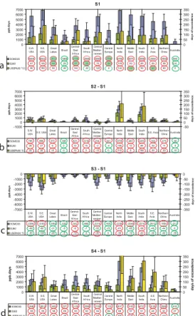
As shown in Fig. 3, elevated values for the SOMO35, EU60, and USEPA80 indices are found in, e.g., the southern U.S., southern Europe, the Middle East and Southeast Asia,

(22)

ACPD

Full Screen / Esc

EGU

exposing the population to health risk. Since the three indices are based on different thresholds, a different geographical pattern is obtained for the three indices. SOMO35 has high values in the southern parts of the U.S., southern Europe, central West Africa and southern parts of the Asian continent. The EU60 and USEPA80 indices typically display high indices in the same areas but with larger variations and gradients. The 5

EU60 ozone threshold is exceeded over larger areas than the USEPA80 threshold, e.g. the EU60 threshold for health risk is exceeded in central Europe, whereas the USEPA80 index is within recommended thresholds. The high values of USEPA80 seen in Fig. 3 (bottom panel) above Africa and South America are associated with biomass burning.

10

As illustrated in Fig. 4a, the EU60 and USEPA80 threshold values are surpassed in most of the 14 selected regions. According to our ensemble model calculations, the EU60 threshold is exceeded in the southeastern U.S. during 105±58 days and the USEPA80 threshold during 19±18 days. Other regions at risk are southern India and the central Mediterranean. Of the 14 selected regions, only Australia has EU60 15

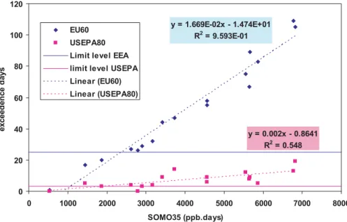
and USEPA80 indices below the recommended thresholds. The highest SOMO35 in-dex of 6.8×103nmol/mol.days is found in the southeastern U.S. The Central Mediter-ranean, northern India, southern India and the Middle East all have values exceeding 5×103nmol/mol.days. Relatively high values are also found in the southwestern U.S., southeastern Asia and northern China. Australia and Latin America are the only an-20

alyzed regions with SOMO35 indices lower than 2.5×103nmol/mol days. In Fig. 5 we present a regression analysis of the regionally averaged data presented in Figure 4a. Interestingly we find a high correlation (r2_{=0.96) of SOMO35 and EU60 in the world} regions; a similar relationship is found for SOMO35 and USEPA80, however statisti-cally less significant (r2=0.55). The SOMO35 threshold level corresponding to EU60 is 25

2.4×103nmol/mol days; the corresponding threshold of SOMO35 with USEPA80 would be 19.5×103nmol/mol days. No limit values have been established for SOMO35 but in the following analysis we use a threshold of 2.4×103nmol/mol days as consistent with both air quality indicators. We note here that these relationships probably hold only for

(23)

ACPD

Full Screen / Esc

EGU

the integrated ozone values in polluted regions as used in this study. These regions are exposed to background ozone levels around 35 nmol/mol with pollution episodes above this level.

As most of the 14 regions exceed the threshold values of EU60 (25 days), USEPA80 (3 days) or SOMO35 (2.4×103nmol/mol days), we explored the extent to which these 5

regions would comply if the regulations would be less stringent. Figure 4a also in-dicates the regions where threshold values are exceeded by less than a factor of 2 (i.e. for EU60 indices >50 days, for USEPA80 indices >6 days, and for SOMO35 in-dices >4.8×103nmol/mol days). Still most regions would not comply with the stan-dards; whereas only the American Great Lakes, central East Africa and central Europe 10

would comply with EU60. It is difficult to assess what the consequences for the air quality indicators would be if indeed the models do systematically overestimate ozone as indicated in Sect. 4.2 and 4.3, since the limited amount of measurements precludes the analysis of the underlying reasons for the overestimates. As a first order analysis we estimate that for instance for the Mediterranean a correction of an annual aver-15

age bias of 10 nmol/mol would bring almost all model calculated ozone air quality to compliance with SOMO35, EU60 and EPA80. In contrast for northern India, almost all models still indicate exceedance of ozone above the thresholds after correcting their annual average by 10 nmol/mol.

We further note that the standard deviations for the computed EU60 indices and es-20

pecially USEPA80 indices are much larger than for SOMO35 indices. This reflects the higher consistency amongst the models in prediction of average ozone levels exceed-ing background values and the larger uncertainty connected with prediction of peak ozone levels. Therefore SOMO35 indices seem to be the most robust indicator for ozone air quality derived from our ensemble of global model calculations. Changes in 25

the three air quality indices over the 14 selected regions for the future cases S2, S3, and S4 will be discussed in Sect. 5.2.

(24)

ACPD

Full Screen / Esc

EGU

5.1.2 Vegetation

Figure 6 shows the model ensemble mean AOT40 for the baseline scenario (S1) considering a growing season of 3 months (AOT403 m) for crops and 6 months (AOT40_{6 m}) for forests, respectively. We further show SUM06 accumulated both over 24 h (SUM0624 h) and daylight hours only (SUM06day), and W126 indices. Figure 7a 5

displays the ensemble mean weighted averages and standard deviations of these in-dices for the 14 selected regions.

Similarly to the health indices, ‘hot spots’ with elevated values in the vegetation indices are found in industrialized areas of Europe, the U.S. and Asia as well as in biomass burning areas in Latin America and Africa. The 5 vegetation indices in 10

the 14 selected regions show high mutual correlation coefficients, between r2=0.85 (AOT406 mvs. SUMO624 h) and r

2

=0.99 (SUM0624 hvs. W126). The AOT40 ensemble means show lower standard deviations than SUM06 and W126, confirming the higher consistency amongst the models when predicting exceedance of concentrations closer to background ozone levels compared to exceedance of high ozone levels.

15

AOT40_{3 m} indices larger than 20×103nmol/mol h are predicted over the central Mediterranean, the southeastern U.S., the Middle East and northern India. The low-est values are found over Australia and Latin America. Only in Australia AOT403 mis below the critical level (the level below which adverse effects would not be expected to occur, i.e. 3×103nmol/mol h for agricultural crop). When we calculate the same 20

AOT403 m solely based on the set of observations given in Sect. 4.2, we calculate for central Europe and the central Mediterranean AOT40 of 9.4±2.8×103nmol/mol h and 13.0±6.5×103nmol/mol h, respectively. The corresponding model ensemble values of 10.3±5.9×103nmol/mol h are consistent for central Europe. However, the computed 23.2±10.7×103nmol/mol h for the central Mediterranean is a factor of two higher, show-25

ing the large sensitivity of AOT40 to accurate calculations of ozone around 40 nmol/mol. A further factor in explaining the discrepancies over the Mediterranean area may be lack of model resolution to resolve the difference of ozone over land and sea as we

(25)

ACPD

Full Screen / Esc

EGU

average out the highly different mixing depths and deposition velocities between ocean and land.

We calculate AOT406 m (forests, 6 months) of more than 30×10 3

nmol/mol h for the southwestern and southeastern U.S., the central Mediterranean, and the Middle East; i.e. 6 times the exceedance of the critical level for reduction of forest growth 5

(5×103nmol/mol h). Of the 14 regions, only Australia has AOT406 m lower than this threshold. The calculated SUM0624 h and SUM06day are very similar with in general differences less than 10%, and exceed 50×103nmol/mol h over the southeastern U.S., the central Mediterranean, northern India and the Middle East and have the lowest value over Australia. As opposed to AOT40 and SUM06, the W126 index uses a con-10

tinuous weighting function. However, W126 correlates very well with AOT403 m and SUM06day. The highest W126 values are found in the central Mediterranean, the south-eastern U.S., India and the Middle East (exceeding 40×103nmol/mol h) whereas the lowest values are found over Australia, Latin America and central Europe. As shown in Sect. 3.2, limit levels of 13×103nmol/mol h for SUM06day and 9×10

3

nmol/mol h for 15

W126 would correspond to a 5% yield loss.

For the reference case S1 in all regions except Australia these limits are exceeded, indicating the potential for significant crop losses due to ozone pollution.

5.2 Year 2030, future scenarios 5.2.1 Health

20

The current legislation scenario (CLE) implies a general increase in the computed health-based pollution indices, with highest increases in the NH and in particular over the Indian sub-continent. Regional average changes are presented for the 14 selected regions in Fig. 4b. The SOMO35 index increases by 23% in the NH and by 15% in the SH. We note that previous numbers are surface area averaged, and not weighted 25

(26)

ACPD

Full Screen / Esc

EGU

nmol/mol.days.

The increase of background ozone (as indicated by the SOMO35 index) is in general paired with increased peak ozone values (indicated by EU60 and USEPA80 indices). Averaged over the continental NH, the EU60 index increases by 47% while the SH is subject to a smaller change of 12%. The change is not uniformly distributed: we 5

find the largest increase in 2030 over India with approximately 100 additional days of exceedance, a doubling compared to S1. Opposed to the general trend, there is a small decrease in EU60 over the Central Mediterranean (−3%) and central Europe (−15%) bringing Central European values below the threshold for health risk.

For USEPA80, we also find large increases over the Indian sub-continent, amounting 10

to 320% and 400% over northern India and southern India, respectively, giving totals of 34 and 27 days of excess. European values are lowered, with 9 days of exceedance for the Central Mediterranean and central European values below the threshold for health risk.

Europe is an interesting policy relevant case: according to the conventional EU60 15

and USEPA80 indices, air quality is improved under the CLE scenario, due to reduc-tions in domestic anthropogenic emissions. However, the European SOMO35 index increases, reflecting a continued rise in European background ozone values due to the increased global emissions of ozone precursors and intercontinental transport. Simi-larly, a rise in surface ozone in the U.S. despite domestic reductions was calculated by 20

Fiore et al. (2002) for the year 2030 based on the IPCC A1 and B1 scenarios. This is contradictory to the general SOMO35 – EU60 correlation established before, showing that the change of indices is not necessarily coupled in all cases. Following our previ-ous analysis, in 2030 CLE the “2x threshold” is exceeded in 12, 11, and 11 regions for SOMO35, EU60, and USEPA80, respectively. The relatively “clean” regions are mostly 25

limited to the extra-tropics, where photochemistry is less intense. Future work should consider the potential discrepancy of models with measurements.

The maximum feasible reduction scenario (MFR) leads to a worldwide improvement of ozone air pollution. Regional averages of change are presented in Fig. 4c, and

(27)

ACPD

Full Screen / Esc

EGU

the global distribution is shown in Fig. 8a and c. The largest reductions appear in polluted areas, i.e. southern parts of the U.S., southern Europe, the Middle East, India and S.E. Asia in response to reduced anthropogenic emissions of ozone precursors. Under the MFR scenario ozone is below or close to the respective thresholds. We note, however, that in our study we did not assume that biomass burning emissions would 5

decrease. A reduction of emissions as indicated by the MFR scenario has a positive effect on future surface ozone levels; the general compliance to all three health indices clearly demonstrates the capacity for this emission scenario to abate ozone pollution and thereby reduce undesirable health effects.

The SRES A2 scenario raises the health-based ozone pollution indices worldwide, 10

especially over industrialized regions (Figs. 4d, 8b, and d). The area with elevated val-ues extends further into northern Europe, northern Asia and Africa. Both background ozone and peak ozone episodes increase, but with a relatively stronger increase in peak ozone episodes, giving continental NH values of 5.6×103nmol/mol days for the SOMO35 index (75% increase), 81 days for the EU60 index (153% increase) and 16 15

days for the USEPA80 index (300% increase). In the Indian subcontinent we find air quality indices higher than anywhere else in the world, but as we noted before, models tend to overestimate ozone in that region. Very high values are also found over North America, e.g. 9.4×103nmol/mol days (SOMO35), 164 days of exceedance (EU60) and 48 days of exceedance (USEPA80) over the southeastern U.S. Also in the central 20

Mediterranean, the Middle East and southeast Asia we find high values, i.e. SOMO35 index of approximately 8×103nmol/mol days, the EU60 threshold exceeded on approx-imately 100 days and USEPA80 threshold values being exceeded on more than 30 days.

In particular, the increase in number of days exceeding 80 nmol/mol (USEPA80) over 25

the Indian sub-continent and the Middle East is prominent. The large increase in the number of days exceeding 60 nmol/mol over Australia is probably due to transport of pollution from southern Asia. The increase in the SOMO35 index is largest over Latin America, the African regions and India. The EU60 and USEPA80 thresholds for health

(28)

ACPD

Full Screen / Esc

EGU

risk are largely surpassed in all regions and on a global average, demonstrating an alarming development if emissions rise as anticipated in the A2 scenario. West et al. (2006, 2007) have related elevated ozone concentrations until 2030 to global pre-mature mortalities for the case of possible methane mitigation and the IIASA emission scenarios.

5

5.2.2 Vegetation

Figure 7b, c, and d show the changes in exceedance of all vegetation air quality indices for CLE, MFR and A2, respectively, for the 14 selected regions. Figure 9 illustrates the geographical distributions of the change (shown are AOT40_{3 m}and SUM06_dayfor crops, AOT406 mfor forests) for MFR and SRES A2, i.e. the low and the high emission cases, 10

contrasting what is possible with today’s technology and what is estimated to happen without further regulation.

As expected, CLE leads to a general increase in the exceedance of vegetation indices in the year 2030, and according to all indicators in all regions, except Aus-tralia, crop losses larger than 5% occur (i.e. larger than 3.0×103, 9.0×103, and 15

12.0×103nmol/mol h for AOT40, SUMO6 and W126).

The increase over the NH for the vegetation indices ranges between 21–38%. On the Indian subcontinent, where no restrictive measures on emissions of ozone precur-sors were assumed to be implemented, the AOT40 indices increase 50–63%, whereas the SUM06 and W126 indices increase by 75–97%. This indicates a larger increase 20

in episodic peak levels compared to the increase in ozone background levels in this region. Large increases are also found in S.E. Asia where increases in emissions from transport and power generation are anticipated, i.e. 20–30% for AOT40 and 30–40% for SUM06 and W126.

Increases of the same order are also found over the African regions due to increased 25

biofuel use. Despite the implementation of policies for air quality improvement, the selected U.S. regions show an increase between 20 and 30% for SUM06 and W126 (i.e. the U.S. favored indices) and between 12 and 16% for AOT40. In contrast, currently

(29)

ACPD

Full Screen / Esc

EGU

implemented European legislation stabilizes or slightly reduces the vegetation indices over Europe by 2030. In particular, the central Mediterranean is the only region (out of the 14) where all indices show a decreasing trend. In agreement with the findings for the health air quality indices, we find larger reductions over Europe for indices based on higher threshold values (SUM06 and W126) than for the lower threshold AOT40 5

indices.

The MFR scenario leads to a worldwide decrease of the vegetation indices. The reductions appear in polluted areas with the largest reductions in southern parts of the U.S., Europe, the Middle East, northern China and Southeast Asia, i.e. AOT40 de-crease by 50–70%, SUM06 and W126 by 70–200% in these regions. Nevertheless, in 10

most regions the MFR emission reductions do not bring AOT40 values below the critical level for agricultural crops (3×103nmol/mol h) or forests (5×103nmol/mol h), confirmed by the results of SUM06 and W126.

The SRES A2 scenario leads to large worldwide increases in the vegetation in-dices and in particular over industrialized regions. The largest increases are found in 15

Southeast Asia and India where AOT40 increases by 80–100%, SUM06 and W126 by 90–160%. Very high levels are found over India, the Middle East, Southeast Asia, U.S., central Mediterranean and northern China/Japan, e.g. AOT40 values in the U.S. and the central Mediterranean exceed 40×103nmol/mol h, SUM06 and W126 reach 95×103nmol/mol h. With the exception of Australia, ozone in all regions is now 20

well above the threshold for damaging sensitive vegetation. 5.3 Climate-air quality interactions

A preliminary analysis of climate-air quality interactions was made based on three chemistry-climate models (MOZECH, MOZART4 and CHASER GCM) that provided hourly surface ozone concentrations for the calculation of ozone indices. Figure 10 25

shows changes in exceedances of EU60, USEPA80, and SOMO35 from scenario S2 to S5, i.e. isolating the climate change effect. The MOZECH model yields much higher exceedances for the U.S. and Europe, while over India it is much lower in the S5

(30)

sce-ACPD

Full Screen / Esc

EGU

nario. Large effects are also modeled by the MOZART4 model, with large reductions of exceedances over India and China/Japan, especially for the SOMO35 and EU60 indices, indicating a change of background ozone. By and large, the CHASER model calculates smaller effects than the other two models. However, as is obvious from Fig. 10 it must be stressed that the spread between the models is large and there 5

is disagreement even on sign, so that the results must be considered as inconclu-sive. Future work on the interaction of climate change and ozone should focus on separating out the effects leading to the ozone changes, such as changes in humidity, stratosphere-troposphere exchange, and deposition.

6 Summary and conclusions

10

This study represents, to our knowledge, the most extensive evaluation of surface ozone calculated by using an 18-member ensemble of global chemistry transport mod-els. Our analysis focused on a set of 14 world regions, 13 with a high population density and expected high surface ozone, and one background region. Comparison of modeled ozone with measurements from North America, Europe, and a limited num-15

ber of measurements from northern China shows relatively good agreement, mostly within 10 nmol/mol. However, large overestimates of ozone, up to 30 nmol/mol in some seasons, are found for almost all models in Africa, the Middle East and India. Prob-lems with emissions, chemical and meteorological descriptions of the coarse resolution global models may contribute to the discrepancy, but we cannot exclude the possibility 20

that the few measurements available in these regions were not representative. Until more measurements become available model improvement and testing of reasons for discrepancies is precluded. Hourly surface ozone fields from the models were used to estimate health-related air quality indices, since these indices are typically derived from the correlation of results of epidemiological studies with measured hourly sur-25

face ozone concentrations (WHO, 2003). We have considered three health related air quality indices: the recently recommended SOMO35, evaluating ozone