Data-Driven Dynamic Optimization with Auxiliary
Covariates
by
Christopher George McCord
B.S.E., Princeton University (2015)
Submitted to the Sloan School of Management
in partial fulfillment of the requirements for the degree of
Doctor of Philosophy in Operations Research
at the
MASSACHUSETTS INSTITUTE OF TECHNOLOGY
June 2019
c
○ Massachusetts Institute of Technology 2019. All rights reserved.
Author . . . .
Sloan School of Management
May 17, 2019
Certified by . . . .
Dimitris Bertsimas
Boeing Professor of Operations Research
Co-director, Operations Research Center
Thesis Supervisor
Accepted by . . . .
Patrick Jaillet
Dugald C. Jackson Professor, Department of Electrical Engineering and
Computer Science
Co-director, Operations Research Center
Data-Driven Dynamic Optimization with Auxiliary Covariates
by
Christopher George McCord
Submitted to the Sloan School of Management on May 17, 2019, in partial fulfillment of the
requirements for the degree of
Doctor of Philosophy in Operations Research
Abstract
Optimization under uncertainty forms the foundation for many of the fundamental problems the operations research community seeks to solve. In this thesis, we develop and analyze algorithms that incorporate ideas from machine learning to optimize uncertain objectives directly from data.
In the first chapter, we consider problems in which the decision affects the observed outcome, such as in personalized medicine and pricing. We present a framework for using observational data to learn to optimize an uncertain objective over a continuous and multi-dimensional decision space. Our approach accounts for the uncertainty in predictions, and we provide theoretical results that show this adds value. In addition, we test our approach on a Warfarin dosing example, and it outperforms the leading alternative methods.
In the second chapter, we develop an approach for solving dynamic optimization problems with covariates that uses machine learning to approximate the unknown stochastic process of the uncertainty. We provide theoretical guarantees on the effec-tiveness of our method and validate the guarantees with computational experiments. In the third chapter, we introduce a distributionally robust approach for incor-porating covariates in large-scale, data-driven dynamic optimization. We prove that it is asymptotically optimal and provide a tractable general-purpose approximation scheme that scales to problems with many temporal stages. Across examples in ship-ment planning, inventory manageship-ment, and finance, our method achieves improve-ments of up to 15% over alternatives.
In the final chapter, we apply the techniques developed in previous chapters to the problem of optimizing the operating room schedule at a major US hospital. Our partner institution faces significant census variability throughout the week, which limits the amount of patients it can accept due to resource constraints at peak times. We introduce a data-driven approach for this problem that combines machine learning with mixed integer optimization and demonstrate that it can reliably reduce the maximal weekly census.
Title: Boeing Professor of Operations Research Co-director, Operations Research Center
Acknowledgments
As my time at grad school comes to a close, I cannot help but feel incredibly fortunate to have had the opportunity to study at MIT. The past four years have certainly helped shape the trajectory of my life, both professionally and personally.
I owe a special thanks to my advisor, Dimitris, who has been an important mentor and has helped me mature as a researcher. He has often accused me of being overly reserved in my opinions, so let me explicitly express that I admire his passion for impacting the world through research and respect his genuine concern for the well-being of all of his students.
I am lucky that Vivek Farias and Colin Fogarty were both willing to serve on my thesis committee. They provided very helpful feedback and challenged me in ways that forced me to better understand the problems I was working on. In addition, I am grateful that Colin served on my general exam committee, along with John Tsitsiklis. Their comments helped me strengthen Chapter 3. I am also grateful for Rahul Mazumder, who has answered all of my questions about computational statistics over the past few years. I developed a much stronger understanding thanks to his patience. In addition, I owe thanks to Roy Welsch, who advised me and provided funding for me during my first year.
My thesis would not have been possible without the ORC administrative staff, Laura Rose, Andrew Carvalho, and Nikki Fortes, who have all been friendly and helpful in addressing my numerous questions and requests.
I am grateful for my collaborators, both internal and external. Brad Sturt, who worked with me on Chapter 4, constantly pushed me to explain my thought process clearly, and my understanding of the problem, as well as my writing, improved as a result. Martin Copenhaver worked with me on Chapter 5, and I benefited significantly from his deep understanding of the healthcare industry, as well as his impressive work ethic. I also collaborated with Nishanth Mundru on several projects, and I am grateful for his extensive knowledge of the literature and his attention to detail. In addition, Chapter 5 would not have been possible if not for my external collaborators at Beth
Israel Deaconess Medical Center, especially Manu and Ryan.
I was very fortunate to serve as a teaching assistant for classes taught by Rob Freund and Caroline Uhler. Both are outstanding lecturers, and I learned a lot by observing them teach. In addition, both provided me with important mentorship during my early years of grad school. I am also blessed to have had the mentorship and spiritual guidance of Father Dan Moloney, the TCC chaplain, throughout the past four years. Father Dan consistently provided insightful analysis of Scripture and highlighted its relevance to issues in the lives of students.
When I first started at MIT, I did not expect to develop many lasting friendships, but I am extremely lucky to have been surrounded by some incredible people in the ORC. Yeesian Ng has been a great friend throughout my four years in grad school. In addition to teaching me a significant amount about robust optimization, he also gave me very helpful feedback on my defense presentation. I’m glad I got to know him through both the ORC and the TCC. Jourdain Lamperski has also been a great friend, and I admire his creativity and passion for research. He has outstanding geometric intuition about problems, and I’ve learned a lot from him. He’s also really entertaining to be around, and I’ve enjoyed getting to know him and his wife, Lauren. I am very grateful for my friendship with Scott Hunter. Scott has an incredible work ethic and the humility to constantly push himself to be better in all aspects of life. I’m lucky to call him a friend because he pushes me to be better as well.
My work over these past four years would never have been possible without the support of my friends and family. I was very fortunate to have a few amazing friends in my life during my time as an undergrad, and I am even more fortunate to still have them in my life today. Finally, I cannot possibly express fully my gratitude for the support and sacrifices of my family. My brother, my mom, and my dad have always taken interest in my work and have consistently encouraged me in all areas of my life, and, for that, I am eternally grateful.
Contents
1 Introduction 15
1.1 Background . . . 16
1.2 Contributions . . . 18
2 Optimization over Continuous and Multi-Dimensional Decisions with Observational Data 23 2.1 Introduction . . . 23
2.1.1 Notation . . . 25
2.1.2 A Motivating Example for Uncertainty Penalization . . . 26
2.1.3 Related Work . . . 28 2.1.4 Contributions . . . 30 2.2 Approach . . . 30 2.2.1 Parameter Tuning . . . 32 2.3 Theory . . . 33 2.3.1 Tractability . . . 36 2.4 Results . . . 37 2.4.1 Pricing . . . 37 2.4.2 Warfarin Dosing . . . 38 2.5 Conclusions . . . 41
3 From Predictions to Prescriptions in Multistage Optimization Prob-lems 43 3.1 Introduction . . . 43
3.1.1 Multistage Optimization and Sample Average Approximation . 45
3.1.2 Related Work . . . 46
3.1.3 Contributions and Structure . . . 48
3.2 Approach . . . 49
3.2.1 Notation . . . 51
3.3 Asymptotic Optimality . . . 52
3.3.1 𝑘-Nearest Neighbor Weight Functions . . . 53
3.3.2 CART Weight Functions . . . 60
3.3.3 Random Forest Weight Functions . . . 68
3.4 Finite Sample Guarantees . . . 70
3.5 Computational Examples . . . 78
3.5.1 Multistage Inventory Control . . . 78
3.5.2 Multistage Lot Sizing . . . 81
3.6 Conclusion . . . 83
4 Sample Robust Optimization with Covariates 85 4.1 Introduction . . . 86
4.1.1 Contributions . . . 87
4.1.2 Comparison to Related Work . . . 89
4.2 Problem Setting . . . 91
4.2.1 Notation . . . 92
4.3 Sample Robust Optimization with Covariates . . . 93
4.3.1 Preliminary: Sample Robust Optimization . . . 93
4.3.2 Incorporating covariates into sample robust optimization . . . 94
4.4 Asymptotic Optimality . . . 96
4.4.1 Main result . . . 96
4.4.2 Review of the Wasserstein metric . . . 98
4.4.3 Concentration of the weighted empirical measure . . . 99
4.4.4 Proof of main result . . . 106
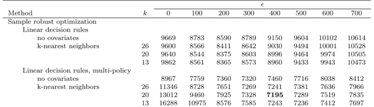
4.6 Computational Experiments . . . 109
4.6.1 Shipment planning . . . 110
4.6.2 Dynamic inventory management . . . 113
4.6.3 Portfolio optimization . . . 116
4.7 Conclusion . . . 118
5 Data-Driven Optimization of Operating Room Blocks 119 5.1 Introduction . . . 119
5.1.1 Related work . . . 122
5.1.2 Contributions and Structure . . . 124
5.2 Problem Formulation and Deterministic Approach . . . 125
5.3 Data-driven Approach . . . 129
5.3.1 Review of predictive-to-prescriptive analytics framework . . . 129
5.3.2 Data-driven OR scheduling formulation . . . 132
5.4 Application and Impact . . . 136
5.4.1 Results . . . 136
5.4.2 Extension for Targeted Growth . . . 138
5.5 Conclusion . . . 139
6 Conclusion 141 A Appendix for Chapter 2 143 A.1 Proofs . . . 143
A.2 Optimization with Linear Predictive Models . . . 152
A.3 Data Generation . . . 153
A.3.1 Pricing . . . 153
A.3.2 Warfarin Dosing . . . 154
A.4 Sensitivity to Selection of Tuning Parameters . . . 155
B Appendix for Chapter 3 157 B.1 Additional Results on Random Forest Weight Functions . . . 157
C Appendix for Chapter 4 167
C.1 Properties of Weight Functions . . . 167
C.2 Proofs from Section 4.4.4 . . . 171
C.3 Technical Details for Section 4.5 . . . 177
C.3.1 Proof of Theorem 4.3 . . . 177
C.3.2 Compact representation of multi-policy approximation . . . . 178
List of Figures
2-1 Regret of two methods as a function of the number of training sam-ples, 𝑛. PCM=Predicted cost minimization, UP-PCM=Uncertainty penalized predicted cost minimization. . . 27 2-2 Comparison of relevant methods on a pricing example and a Warfarin
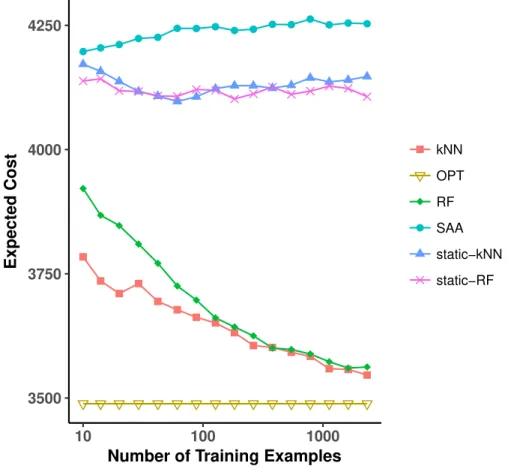
dosing example. . . 38 3-1 Out of sample results with various weight functions for a twelve stage
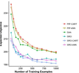
inventory control problem. Vertical axis represents expected cost of policy (smaller is better). . . 80 3-2 Average out-of-sample cost of policies computed using various weight
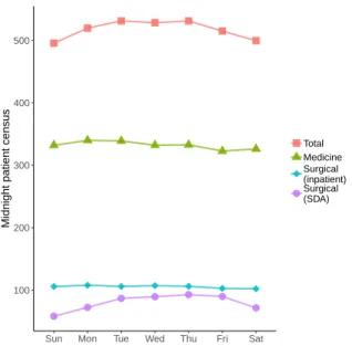
functions for twelve stage lot sizing problem. Horizontal axis shows number of training examples. . . 82 4-1 Out-of-sample profit for the shipment planning example. . . 112 4-2 Out-of-sample objective for the portfolio optimization example. . . . 118 5-1 Average overnight census by day of the week. . . 121 5-2 Out-of-sample reduction in average maximum weekly census for each
of the various models. . . 138 A-1 Effect of 𝜆 tuning on the random forest method for Warfarin example 156
List of Tables
3.1 Summary of notation. . . 52
4.1 Relationship of four methods. . . 109
4.2 Statistical significance for shipment planning problem. . . 112
4.3 Average out-of-sample cost for dynamic procurement problem. . . 114
4.4 Statistical significance for dynamic procurement problem. . . 115 4.5 Average computation time (seconds) for dynamic procurement problem. 115
Chapter 1
Introduction
Optimization under uncertainty forms the foundation for many of the the fundamental applications the operations research community seeks to solve. A retailer managing inventory levels, an investor allocating money, a hospital scheduling resources, and a physician prescribing treatments all face problems that share the same characteristics. Each aims to make a decision to optimize an objective function that depends on an uncertain quantity. The retailer faces uncertain future demand when deciding how much inventory to order to maximize profit. The investor faces uncertain future returns when trying to construct a portfolio with an optimal risk-reward tradeoff. The hospital faces unknown future demand for services when creating its operating room schedule. The physician faces uncertainty in how the patient will respond when prescribing a treatment to minimize adverse effects.
Formally, we model the uncertainty in each of these problems as a random variable with an unknown distribution. In practice, decision makers have access to data con-sisting of past realizations of the uncertainty, so we aim to learn to make near-optimal decisions from this data. In addition, decision makers often have access to auxiliary covariates that can help predict future uncertainty. For example, the retailer has data on market trends and social media interest that can help predict future demand, and the physician knows demographic and genetic factors that can help predict how a pa-tient will respond to specific treatments. The covariates provide valuable information for the decision-maker, but it is not always clear how to efficiently use them. Many
effective machine learning methods exist for using covariates to make point predic-tions. However, learning to make good decisions presents a greater challenge because it often requires an understanding of the distribution of the uncertainty rather than just a point prediction. In this thesis, we develop and analyze data-driven algorithms that incorporate ideas from machine learning in order to solve optimization problems with auxiliary covariates.
1.1
Background
We now review some existing data-driven approaches to optimization problems with covariates. These basic problems are characterized by four components:
∙ Decision: 𝑧 ∈ 𝒵 ⊂ R𝑑𝑧,
∙ Uncertainty: 𝑌 ∈ 𝒴 ⊂ R𝑑𝑦,
∙ Cost function: 𝑐 : 𝒵 × 𝒴 → R, ∙ Auxiliary covariates: 𝑋 ∈ 𝒳 ⊂ R𝑑𝑥.
For a newly observed vector of auxiliary covariates, 𝑥 ∈ 𝒳 , we want to find a decision that minimizes the conditional expected cost,
min
𝑧∈𝒵 E[𝑐(𝑧; 𝑌 ) | 𝑋 = 𝑥]. (1.1)
While we do not know the conditional distribution of 𝑌 given 𝑋, we do have access to data consisting of 𝑁 observations,
(𝑥1, 𝑦1), . . . , (𝑥𝑁, 𝑦𝑁).
One approach to solving (1.1) is sample average approximation (SAA). In this ap-proach, we replace the unknown distribution of 𝑌 with the empirical distribution of
the training data, resulting in the following problem: min 𝑧∈𝒵 1 𝑁 𝑁 ∑︁ 𝑖=1 𝑐(𝑧; 𝑦𝑖).
Despite its simplicity SAA produces asymptotically optimal decisions for (1.1) if 𝑌 is independent of the covariates 𝑋 (under mild technical conditions on 𝒵 and 𝑐). In other words, if the covariates provide no information on the uncertainty, then the optimal decisions for the SAA problem converge to optimal decisions of (1.1) as the number of training samples goes to infinity. For more details, see Shapiro et al. [89]. A key limitation of SAA is that it ignores the covariates, so when 𝑋 provides information about 𝑌 , it may produce decisions that are asymptotically suboptimal for (1.1). Bertsimas and Kallus [15] propose a modified approach in which they replace the unknown distribution of 𝑌 by a weighted empirical distribution,
min 𝑧∈𝒵 𝑁 ∑︁ 𝑖=1 𝑤𝑖𝑁(𝑥)𝑐(𝑧; 𝑦𝑖), (1.2) where 𝑤𝑁 : 𝒳 → R𝑁 is a weight function. Many choices of weight functions exist, but, intuitively, for each 𝑖 ∈ {1, . . . , 𝑁 }, 𝑤𝑁
𝑖 (𝑥) should measure the similarity between
the new covariate vector, 𝑥, and the covariate vector of the 𝑖th training example, 𝑥𝑖. Bertsimas and Kallus [15] list several examples, including the 𝑘-nearest neighbor weight function, 𝑤𝑁,kNN𝑖 (𝑥) := ⎧ ⎪ ⎨ ⎪ ⎩ 1 𝑘, 𝑥
𝑖 is a 𝑘-nearest neighbor of 𝑥 out of {𝑥1, . . . , 𝑥𝑁},
0, otherwise,
where 𝑘 ∈ N, and the kernel regression weight function, 𝑤𝑁,𝐾𝑅𝑖 (𝑥) := 𝐾(︂ ‖𝑥
𝑖− 𝑥‖
ℎ )︂
,
where ℎ > 0 is a bandwidth parameter and 𝐾(·) is a kernel function (such as the Gaussian kernel, 𝐾(𝑢) = √1
2𝜋𝑒 −𝑢2/2
inspired by classification and regression trees (CART) and random forests. We will discuss these further in later chapters.
All of the above-mentioned weight functions are inspired by nonparametric ma-chine learning methods. These nonparametric methods have proven effective at pre-diction because they can learn complex relationships between the covariates and the response variable without requiring the practitioner to know an explicit parametric form. Similarly, Bertsimas and Kallus [15] show that, under appropriate conditions, optimal decisions for (1.2) with these weight functions are asymptotically optimal for (1.1), without any parametric assumptions on the relationship between 𝑋 and 𝑌 . In other words, incorporating covariates via a nonparametric weight function in (1.2) can lead to asymptotically better decisions than SAA, even without specific knowledge of how the covariates affect the uncertainty.
1.2
Contributions
This thesis extends the approach in (1.2) along several dimensions. In particular, we consider observational optimization problems in which the decision, 𝑧, affects the observation of the uncertainty, 𝑌 . This occurs in several important applications, such as personalized medicine and pricing. We also consider dynamic optimization prob-lems, which consist of a series of temporal stages. In each stage, 𝑡 ∈ {1, . . . , 𝑇 }, the decision maker chooses a decision 𝑧𝑡 and then observes uncertainty 𝑌𝑡. For example,
consider the retailer managing its inventory of a product. Each week, the retailer observes the current inventory level and decides how much to order for the following week. Crucially, the retailer bases its decision on the remaining inventory level at that time, which depends on the realizations of demand in past weeks. Therefore, in dynamic problems, the decision in each stage is not a fixed quantity, but rather a function of the uncertainty revealed by that point in time. We develop and analyze approaches to these problems in the following chapters.
Optimization over Continuous and Multi-dimensional Decisions
with Observational Data
In Chapter 2, we consider observational optimization problems. The data in this case consists of tuples of covariates, decision, and uncertainty, (𝑥1, 𝑧1, 𝑦1), . . . , (𝑥𝑁, 𝑧𝑁, 𝑦𝑁).
This setting introduces two challenges not present in the basic setting of (1.1). First, the data is incomplete. We do not observe what the realization of the uncertainty would have been under a different decision. Second, there may be confounding be-tween 𝑧 and 𝑦 in the training data. We address these challenges with a method that not only predicts the cost of each potential decision, but also estimates the variance of those predictions. Accounting for the variance of the predicted cost adds signifi-cant value when the decision space, 𝒵, is continuous or multidimensional and there are many potential decisions. We establish this through both theoretical and com-putational results. As an example, we consider the problem of personalized Warfarin dosing, in which the decision, 𝑧, is the dose assigned to the patient, the uncertainty, 𝑌 , is the response of the patient, as measured by the international normalized ratio, and the covariates for each patient, 𝑋, include demographic information, medical history, and the genotype variant at certain sites. We compare our method against alternatives on real data and find that our approach obtains the best out-of-sample performance across all sizes of training sets.
From Predictions to Prescriptions in Multistage Optimization
Problems
In Chapter 3, we consider 𝑇 -stage dynamic optimization problems with covariates. We assume that, in addition to the uncertainty, 𝑌 , evolving over time, the covariates, 𝑋, also evolve over time. The decision maker must take into account this additional available information when making decisions. We introduce a data-driven approach to these dynamic problems that uses machine learning to define a stochastic process with finite support that approximates the true stochastic process of the uncertainty, (𝑌1, . . . , 𝑌𝑇). We can solve the resulting problem with techniques from dynamic
pro-gramming and approximate dynamic propro-gramming (see Bertsekas [11] for reference). We prove that the decisions produced by our approach are asymptotically optimal un-der mild, nonparametric conditions, and we establish finite sample guarantees on the optimality gap. We validate this theory with computational results on two inventory management examples.
Sample Robust Optimization with Covariates
In Chapter 4, we again consider 𝑇 -stage dynamic optimization problems with covari-ates. However, instead of approximating the stochastic process of the uncertainty, we introduce robustness to (1.2) and optimize over decision rules. A decision rule is a collection of functions that specify what decision to make in each stage based on the information revealed up until that point. For the example of the retailer, a decision rule for week 𝑡 specifies an ordering quantity as a function of the observed demands from weeks 1, . . . , 𝑡 − 1. We establish that our approach produces asymptotically optimal decision rules. The proof of this relies on a novel result regarding the con-vergence in Wasserstein distance of the weighted empirical distribution introduced in (1.2) to the conditional distribution of the uncertainty given the covariates. We also demonstrate the tractability of the approach by applying it to several computational examples with up to twelve stages.
Data-Driven Optimization of Operating Room Blocks
In Chapter 5, we use the techniques developed in this thesis to optimize the operat-ing room block schedule of a major US hospital. Our partner institution, like many other hospitals, faces significant census variability throughout the week, which limits the amount of patients it can accept due to resource constraints during peak times. To optimize the block schedule to minimize census peaks, we develop a mixed inte-ger optimization approach that employs predictive machine learning to estimate the distributions of surgical patients’ lengths of stay. In addition, by using ideas from Chapter 2, our approach accounts for the impact that moving the date of surgery has
on patients’ lengths of stay. We demonstrate the effectiveness of the approach with simulation results using real data and find that we can reliably reduce the maximal weekly census with only a few changes to the schedule.
Chapter 2
Optimization over Continuous and
Multi-Dimensional Decisions with
Observational Data
In this chapter, we consider the optimization of an uncertain objective over continu-ous and multi-dimensional decision spaces in problems in which we are only provided with observational data. We propose a novel algorithmic framework that is tractable, asymptotically consistent, and superior to comparable methods on example problems. Our approach leverages predictive machine learning methods and incorporates infor-mation on the uncertainty of the predicted outcomes for the purpose of prescribing decisions. We demonstrate the efficacy of our method on examples involving both synthetic and real data sets.
2.1
Introduction
We study the general problem in which a decision maker seeks to optimize a known objective function that depends on an uncertain quantity. The uncertain quantity has an unknown distribution, which may be affected by the action chosen by the decision maker. Many important problems across a variety of fields fit into this framework. In healthcare, for example, a doctor aims to prescribe drugs in specific dosages to
regulate a patient’s vital signs. In revenue management, a store owner must decide how to price various products in order to maximize profit. In online retail, companies decide which products to display for a user to maximize sales. The general problem we study is characterized by the following components:
∙ Decision variable: 𝑧 ∈ 𝒵 ⊂ R𝑝,
∙ Outcome: 𝑌 (𝑧) ∈ 𝒴 (We adopt the potential outcomes framework [83], in which 𝑌 (𝑧) denotes the (random) quantity that would have been observed had decision 𝑧 been chosen.),
∙ Auxiliary covariates (also called side-information or context): 𝑥 ∈ 𝒳 ⊂ R𝑑,
∙ Cost function: 𝑐(𝑧; 𝑦) : 𝒵 × 𝒴 → R. (This function is known a priori.)
We allow the auxiliary covariates, decision variable, and outcome to take values on multi-dimensional, continuous sets. A decision-maker seeks to determine the action that minimizes the conditional expected cost:
min
𝑧∈𝒵 E[𝑐(𝑧; 𝑌 (𝑧))|𝑋 = 𝑥]. (2.1)
Of course, the distribution of 𝑌 (𝑧) is unknown, so it is not possible to solve this problem exactly. However, we assume that we have access to observational data, consisting of 𝑛 independent and identically distributed observations, (𝑋𝑖, 𝑍𝑖, 𝑌𝑖) for
𝑖 = 1, . . . , 𝑛. Each of these observations consists of an auxiliary covariate vector, a decision, and an observed outcome. This type of data presents two challenges that differentiate our problem from a predictive machine learning problem. First, it is incomplete. We only observe 𝑌𝑖 := 𝑌𝑖(𝑍𝑖), the outcome associated with the applied
decision. We do not observe what the outcome would have been under a different decision. Second, the decisions were not necessarily chosen independently of the outcomes, as they would have been in a randomized experiment, and we do not know how the decisions were assigned. Following common practice in the causal inference literature, we make the ignorability assumption of Hirano and Imbens [60].
Assumption 2.1 (Ignorability).
𝑌 (𝑧) ⊥⊥ 𝑍 | 𝑋 ∀𝑧 ∈ 𝒵
In other words, we assume that historically the decision 𝑍 has been chosen as a function of the auxiliary covariates 𝑋. There were no unmeasured confounding variables that affected both the choice of decision and the outcome.
Under this assumption, we are able to rewrite the objective of (2.1) as E[𝑐(𝑧; 𝑌 ) | 𝑋 = 𝑥, 𝑍 = 𝑧].
This form of the objective is easier to learn because it depends only on the observed outcome, not on the counterfactual outcomes. A direct approach to solve this prob-lem is to use a regression method to predict the cost as a function of 𝑥 and 𝑧 and then choose 𝑧 to minimize this predicted cost. If the selected regression method is uniformly consistent in 𝑧, then the action chosen by this method will be asymptot-ically optimal under certain conditions. (We will formalize this later.) However, this requires choosing a regression method that ensures the optimization problem is tractable. For this work, we restrict our attention to linear and tree-based methods, such as CART [30] and random forests [29], as they are both effective and tractable for many practical problems.
A key issue with the direct approach is that it tries to learn too much. It tries to learn the expected outcome under every possible decision, and the level of uncertainty associated with the predicted expected cost can vary between different decisions. This method can lead us to select a decision which has a small point estimate of the cost, but a large uncertainty interval.
2.1.1
Notation
Throughout this chapter, we use capital letters to refer to random quantities and lower case letters to refer to deterministic quantities. Thus, we use 𝑍 to refer to the
decision randomly assigned by the (unknown) historical policy and 𝑧 to refer to a specific action. For a given, auxiliary covariate vector, 𝑥, and a proposed decision, 𝑧, the conditional expectation E[𝑐(𝑧; 𝑌 )|𝑋 = 𝑧, 𝑍 = 𝑧] means the expectation of the cost function 𝑐(𝑧; 𝑌 ) under the conditional measure in which 𝑋 is fixed as 𝑥 and 𝑍 is fixed as 𝑧. We ignore details of measurability throughout and assume this conditional expectation is well defined. Throughout, all norms are ℓ2 norms unless otherwise
specified. We use (𝑋, 𝑍) to denote vector concatenation.
2.1.2
A Motivating Example for Uncertainty Penalization
We start with a simple example in which there are 𝑚 possible decisions. We have data on 𝑛 i.i.d. observations of past decisions and outcomes, (𝑍𝑖, 𝑌𝑖) for 𝑖 = 1, . . . , 𝑛.
For simplicity, there are no auxiliary covariates for this problem, and the decision, 𝑍𝑖, has been chosen independently of the potential outcomes, (𝑌𝑖(1), . . . , 𝑌𝑖(𝑚)) (so
Assumption 2.1 holds).
The goal is to choose 𝑧 to minimize the expected outcome. If 𝜇𝑧 = E[𝑌 (𝑧)] is
known for all 𝑧, the optimal decision is given by: 𝑧* ∈ arg min
𝑧 𝜇𝑧. However, this
mean is unknown, so it must be estimated. We define ˆ𝜇𝑧 =
1 ∑︀
𝑖1{𝑍𝑖 = 𝑧}
∑︀
𝑖1{𝑍𝑖 =
𝑧}𝑌𝑖, the empirical expectation of the outcome under 𝑧. Predicted cost minimization
(PCM) minimizes ˆ𝜇𝑧.
To motivate uncertainty penalization, we note that if we assume the rewards are almost surely bounded, |𝑌 | ≤ 1, an application of Bernstein’s inequality shows that with probability at least 1 − 𝛿,
𝜇𝑧 ≤ ˆ𝜇𝑧+ √︃ 2𝜎2 𝑧ln(𝑚/𝛿) ∑︀ 𝑖1{𝑍𝑖 = 𝑧} + 4 ln(𝑚/𝛿) 3∑︀ 𝑖1{𝑍𝑖 = 𝑧} , ∀𝑧, where 𝜎2
𝑧 = Var(𝑌𝑖(𝑧)). This bound motivates the addition of a term to the objective
that penalizes the uncertainty of the estimate ˆ𝜇𝑧. In this simple example, ˆ𝜇𝑧 is
an unbiased estimator for 𝜇𝑧, with Var(ˆ𝜇𝑧) = E [𝜎𝑧2/
∑︀
𝑖1{𝑍𝑖 = 𝑧}]. The penalty
0.00 0.25 0.50 0.75
100 250 500 1000 2000
Number of Training Examples
Expected Regret
PCM UP−PCM
Figure 2-1: Regret of two methods as a function of the number of training samples, 𝑛. PCM=Predicted cost minimization, UP-PCM=Uncertainty penalized predicted cost minimization.
uncertainty penalized objective: ˆ 𝜇𝜆𝑧 = ˆ𝜇𝑧+ 𝜆 √︃ 1 ∑︀ 𝑖1{𝑍𝑖 = 𝑧} ,
where 𝜆 is a tuning parameter. We note that we could also include the action-dependent variance 𝜎𝑧2 in the penalty term. However, this is typically unknown, and we have observed that estimating it without a homoscedasticity assumption can introduce too much noise for the objective to be effective.
For this experiment, we fix 𝑚 = 100 possible actions, each with a fixed mean response, which was drawn from a standard Gaussian distribution. To construct the training data, at each time step, a decision was chosen uniformly at random from the set of possible decisions and the outcome is the mean response plus noise sampled from a standard Gaussian distribution. The regret of each method was computed and averaged over ten thousand trials for a range of values of 𝑛. We held 𝜆 fixed at 1. Our results are shown in Figure 2-1. Uncertainty penalized empirical risk minimization clearly outperforms predicted cost minimization for small training
sample sizes. However, the level of outperformance decreases as 𝑛 increases.
This example serves to motivate the need for uncertainty penalization, especially when training data is limited. The direct approach of choosing the action with the smallest predicted cost is inefficient because the predicted costs can have different levels of uncertainty associated with them. Figure 2-1 demonstrates that we are better off choosing a decision whose cost we can predict with high confidence, rather than decisions whose costs we know little about.
2.1.3
Related Work
Recent years have seen tremendous interest in the area of data-driven optimization. Much of this work combines ideas from the statistics and machine learning litera-ture with techniques from mathematical optimization. Bertsimas and Kallus [15] developed a framework that uses nonparametric machine learning methods to solve data-driven optimization problems in the presence of auxiliary covariates. They take advantage of the fact that for many machine learning algorithms, the predictions are given by a linear combination of the training samples’ target variables. Kao et al. [67] and Elmachtoub and Grigas [47] developed algorithms that make predictions tailored for use in specific optimization problems. However, they all deal with the setting in which the decision does not affect the outcome. This is insufficient for many appli-cations, such as pricing, in which the demand for a product is clearly affected by the price. Bertsimas and Kallus [16] later studied the limitations of predictive approaches to pricing problems. In particular, they demonstrated that confounding in the data between the decision and outcome can lead to large optimality gaps if ignored. They proposed a kernel-based method for data-driven optimization in this setting, but it does not scale well with the dimension of the decision space. Misic [75] developed an efficient mixed integer optimization formulation for problems in which the pre-dicted cost is given by a tree ensemble model. This approach scales fairly well with the dimension of the decision space but does not consider the need for uncertainty penalization.
overview), which concerns the study of causal effects from observational data. Much of the work in this area has focused on determining whether a treatment has a sig-nificant effect on the population as a whole. However, a growing body of work has focused on learning optimal, personalized treatments from observational data. Athey and Wager [2] proposed an algorithm that achieves optimal (up to a constant factor) regret bounds in learning a treatment policy when there are two potential treatments. Kallus [63] proposed an algorithm to efficiently learn a treatment policy when there is a finite set of potential treatments. Bertsimas et al. [21] developed a tree-based algorithm that learns to personalize treatment assignments from observational data. It is based on the optimal trees machine learning method [13] and has performed well in experiments. Considerably less attention has been paid to problems with a con-tinuous decision space. Hirano and Imbens [60] introduced the problem of inference with a continuous treatment, and Flores [50] studied the problem of learning an opti-mal policy in this setting. Recently, Kallus and Zhou [65] developed an approach to policy learning with a continuous decision variable that generalizes the idea of inverse propensity score weighting. Our approach differs in that we focus on regression-based methods, which we believe scale better with the dimension of the decision space and avoid the need for density estimation.
The idea of uncertainty penalization has been explored as an alternative to em-pirical risk minimization in statistical learning, starting with Maurer and Pontil [73]. Swaminathan and Joachims [91] applied uncertainty penalization to the offline bandit setting. Their setting is similar to the one we study. An agent seeks to minimize the prediction error of his/her decision, but only observes the loss associated with the selected decision. They assumed that the policy used in the training data is known, which allowed them to use inverse propensity weighting methods. In contrast, we assume ignorability, but not knowledge of the historical policy, and we allow for more complex decision spaces.
We note that our approach bears a superficial resemblance to the upper confidence bound (UCB) algorithms for multi-armed bandits (cf. Bubeck et al. [31]). These algorithms choose the action with the highest upper confidence bound on its predicted
expected reward. Our approach, in contrast, chooses the action with the highest lower confidence bound on its predicted expected reward (or lowest upper confidence bound on predicted expected cost). The difference is that UCB algorithms choose actions with high upside to balance exploration and exploitation in the online bandit setting, whereas we work in the offline setting with a focus on solely exploitation.
2.1.4
Contributions
Our primary contribution is an algorithmic framework for observational data driven optimization that allows the decision variable to take values on continuous and mul-tidimensional sets. We consider applications in personalized medicine, in which the decision is the dose of Warfarin to prescribe to a patient, and in pricing, in which the action is the list of prices for several products in a store.
2.2
Approach
In this section, we introduce the uncertainty penalization approach for optimization with observational data. Recall that the observational data consists of 𝑛 i.i.d. obser-vations, (𝑋1, 𝑍1, 𝑌1), . . . , (𝑋𝑛, 𝑍𝑛, 𝑌𝑛). For observation 𝑖, 𝑋𝑖 represents the pertinent
auxiliary covariates, 𝑍𝑖 is the decision that was applied, and 𝑌𝑖 is the observed
re-sponse. The first step of the approach is to train a predictive machine learning model to estimate E[𝑐(𝑧; 𝑌 )|𝑋 = 𝑥, 𝑍 = 𝑧]. When training the predictive model, the feature space is the cartesian product of the auxiliary covariate space and the decision space, 𝒳 × 𝒵. We have several options for how to train the predictive model. We can train the model to predict 𝑌 , the cost 𝑐(𝑍, 𝑌 ), or a combination of these two responses. In general, we denote the prediction of the ML algorithm as a linear combination of the cost function evaluated at the training examples,
ˆ 𝜇(𝑥, 𝑧) := 𝑛 ∑︁ 𝑖=1 𝑤𝑖(𝑥, 𝑧)𝑐(𝑧; 𝑌𝑖).
We require the predictive model to satisfy a generalization of the honesty property of Wager and Athey [97].
Assumption 2.2 (Honesty). The model trained on (𝑋1, 𝑍1, 𝑌1), . . . , (𝑋𝑛, 𝑍𝑛, 𝑌𝑛) is
honest, i.e., the weights, 𝑤𝑖(𝑥, 𝑧), are determined independently of the outcomes,
𝑌1, . . . , 𝑌𝑛.
This honesty assumption reduces the bias of the predictions of the cost. We also enforce several restrictions on the weight functions.
Assumption 2.3 (Weights). For all (𝑥, 𝑧) ∈ 𝒳 × 𝒵, ∑︀𝑛
𝑖=1𝑤𝑖(𝑥, 𝑧) = 1 and for all 𝑖,
𝑤𝑖(𝑥, 𝑧) ∈ [0, 1/𝛾𝑛]. In addition, 𝒳 × 𝒵 can be partitioned into Γ𝑛 regions such that
if (𝑥, 𝑧) and (𝑥, 𝑧′) are in the same region, ||𝑤(𝑥, 𝑧) − 𝑤(𝑥, 𝑧′)||1 ≤ 𝛼||𝑧 − 𝑧′||2.
The direct approach to solving (2.1) amounts to choosing 𝑧 ∈ 𝒵 that minimizes ˆ
𝜇(𝑥, 𝑧), for each new instance of auxiliary covariates, 𝑥. However, the variance of the predicted cost, ˆ𝜇(𝑥, 𝑧), can vary with the decision variable, 𝑧. Especially with a small training sample size, the direct approach, minimizing ˆ𝜇(𝑥, 𝑧), can give a decision with a small, but highly uncertain, predicted cost. We can reduce the expected regret of our action by adding a penalty term for the variance of the selected decision. If Assumption 2.2 holds, the conditional variance of ˆ𝜇(𝑥, 𝑧) given (𝑋1, 𝑍1), . . . , (𝑋𝑛, 𝑍𝑛)
is given by
𝑉 (𝑥, 𝑧) :=∑︁
𝑖
𝑤2𝑖(𝑥, 𝑧)Var(𝑐(𝑧; 𝑌𝑖)|𝑋𝑖, 𝑍𝑖).
In addition, ˆ𝜇(𝑥, 𝑧) may not be an unbiased predictor, so we also introduce a term that penalizes the conditional bias of the predicted cost given (𝑋1, 𝑍1), . . . , (𝑋𝑛, 𝑍𝑛).
Since the true cost is unknown, it is not possible to exactly compute this bias. Instead, we compute an upper bound under a Lipschitz assumption (details in Section 2.3).
𝐵(𝑥, 𝑧) :=∑︁
𝑖
𝑤𝑖(𝑥, 𝑧)||(𝑋𝑖, 𝑍𝑖) − (𝑥, 𝑧)||2.
decision by solving
min
𝑧∈𝒵 𝜇(𝑥, 𝑧) + 𝜆ˆ 1
√︀
𝑉 (𝑥, 𝑧) + 𝜆2𝐵(𝑥, 𝑧), (2.2)
where 𝜆1 and 𝜆2 are tuning parameters.
As a concrete example, we can use the CART algorithm of Breiman et al. [30] or the optimal regression tree algorithm of Bertsimas and Dunn [13] as the predictive method. These algorithms work by partitioning the training examples into clusters, i.e., the leaves of the tree. For a new observation, a prediction of the response variable is made by averaging the responses of the training examples that are contained in the same leaf. 𝑤𝑖(𝑥, 𝑧) = ⎧ ⎪ ⎨ ⎪ ⎩ 1 𝑁 (𝑥,𝑧), (𝑥, 𝑧) ∈ 𝑙(𝑥, 𝑧), 0, otherwise,
where 𝑙(𝑥, 𝑧) denotes the set of training examples that are contained in the same leaf of the tree as (𝑥, 𝑧), and 𝑁 (𝑥, 𝑧) = |𝑙(𝑥, 𝑧)|. The variance term will be small when the leaf has a large number of training examples, and the bias term will be small when the diameter of the leaf is small. Assumption 2.2 can be satisfied by ignoring the outcomes when selecting the splits or by dividing the training data into two sets, one for making splits and one for making predictions. Assumption 2.3 is satisfied with 𝛼 = 0 if the minimum number of training samples in each leaf is 𝛾𝑛and the maximum
number of leaves in the tree is Γ𝑛.
2.2.1
Parameter Tuning
Before proceeding, we note that the variance terms, Var(𝑐(𝑧; 𝑌𝑖) | 𝑋𝑖, 𝑍𝑖), are often
unknown in practice. In the absence of further knowledge, we assume homoscedas-ticity, i.e., Var(𝑌𝑖|𝑋𝑖, 𝑍𝑖) is constant. It is possible to estimate this value by training
a machine learning model to predict 𝑌𝑖 as a function of (𝑋𝑖, 𝑍𝑖) and computing the
mean squared error on the training set. However, it may be advantageous to include this value with the tuning parameter 𝜆1.
parameters are associated with the predictive model). Because the counterfactual outcomes are unknown, it is not possible to use the standard approach of holding out a validation set during training and evaluating the error of the model on that validation set for each combination of possible parameters. One option is to tune the predictive model’s parameters using cross validation to maximize predictive accuracy and then select 𝜆1 and 𝜆2 using the theory we present in Section 2.3. Another option
is to split the data into a training and validation set and train a predictive model on the validation data to impute the counterfactual outcomes. We then select the model that minimizes the predicted cost on the validation set. For the examples in Section 2.4, we use a combination of these two ideas. We train a random forest model on the validation set (in order to impute counterfactual outcomes), and we then select the model that minimizes the sum of the mean squared error and the predicted cost on the validation data. In Appendix A.4, we include computations that demonstrate, for the Warfarin example of Section 2.4.2, the method is not too sensitive to the choice of 𝜆1 and 𝜆2.
2.3
Theory
In this section, we describe the theoretical motivation for our approach and provide finite-sample generalization and regret bounds. For notational convenience, we define
𝜇(𝑥, 𝑧) := E[𝑐(𝑧; 𝑌 (𝑧))|𝑋 = 𝑥] = E[𝑐(𝑧; 𝑌 )|𝑋 = 𝑥, 𝑍 = 𝑧],
where the second equality follows from the ignorability assumption. Before presenting the results, we first present a few additional assumptions.
Assumption 2.4 (Regularity). The set 𝒳 × 𝒵 is nonempty, closed, and bounded with diameter 𝐷.
Assumption 2.5 (Objective Conditions). The objective function satisfies the follow-ing properties:
2. For all 𝑦 ∈ 𝒴, 𝑐(·; 𝑦) is 𝐿-Lipschitz.
3. For any 𝑥, 𝑥′ ∈ 𝒳 and any 𝑧, 𝑧′ ∈ 𝒵, |𝜇(𝑥, 𝑧) − 𝜇(𝑥′, 𝑧′)| ≤ 𝐿||(𝑥, 𝑧) − (𝑥′, 𝑧′)||.
These assumptions provide some conditions under which the generalization and regret bounds hold, but similar results hold under alternative sets of assumptions (e.g. if 𝑐(𝑧; 𝑌 )|𝑍 is subexponential instead of bounded). With these additional as-sumptions, we have the following generalization bound. All proofs are contained in Appendix A.1.
Theorem 2.1. Suppose assumptions 2.1-2.5 hold. Then, with probability at least 1 − 𝛿, 𝜇(𝑥, 𝑧) − ˆ𝜇(𝑥, 𝑧) ≤ 4 3𝛾𝑛 ln(𝐾𝑛/𝛿) + 2 √︀ 𝑉 (𝑥, 𝑧) ln(𝐾𝑛/𝛿) + 𝐿 · 𝐵(𝑥, 𝑧) ∀𝑧 ∈ 𝒵, where 𝐾𝑛 = Γ𝑛(︀9𝐷𝛾𝑛(︀𝛼(𝐿𝐷 + 1 + √ 2) + 𝐿(√2 + 3))︀)︀𝑝.
This result uniformly bounds, with high probability, the true cost of action 𝑧 by the predicted cost, ˆ𝜇(𝑥, 𝑧), a term depending on the uncertainty of that predicted cost, 𝑉 (𝑥, 𝑧), and a term proportional to the bias associated with that predicted cost, 𝐵(𝑥, 𝑧). It is easy to see how this result motivates the approach described in (2.2). One can also verify that the generalization bound still holds if (𝑋1, 𝑍1), . . . , (𝑋𝑛, 𝑍𝑛)
are chosen deterministically, as long as 𝑌1, . . . , 𝑌𝑛 are still independent. Using
Theo-rem 2.1, we are able to derive a finite-sample regret bound. Theorem 2.2. Suppose assumptions 2.1-2.5 hold. Define
𝑧* ∈ arg min 𝑧 𝜇(𝑥, 𝑧), ˆ 𝑧 ∈ arg min 𝑧 𝜇(𝑥, 𝑧) + 𝜆ˆ 1 √︀ 𝑉 (𝑥, 𝑧) + 𝜆2𝐵(𝑥, 𝑧).
If 𝜆1 = 2√︀ln(2𝐾𝑛/𝛿) and 𝜆2 = 𝐿, then with probability at least 1 − 𝛿,
𝜇(𝑥, ˆ𝑧) − 𝜇(𝑥, 𝑧*) ≤ 2 𝛾𝑛 ln(2𝐾𝑛/𝛿) + 4 √︀ 𝑉 (𝑥, 𝑧*) ln(2𝐾 𝑛/𝛿) + 2𝐿 · 𝐵(𝑥, 𝑧*),
where 𝐾𝑛 = Γ𝑛(︀9𝐷𝛾𝑛(︀𝛼(𝐿𝐷 + 1 +
√
2) + 𝐿(√2 + 3))︀)︀𝑝 .
By this result, the regret of the approach defined in (2.2) depends only on the variance and bias terms of the optimal action, 𝑧*. Because the predicted cost is penalized by 𝑉 (𝑥, 𝑧) and 𝐵(𝑥, 𝑧), it does not matter how poor the prediction of cost is at suboptimal actions. Theorem 2.2 immediately implies the following asymptotic result, assuming the auxiliary feature space and decision space are fixed as the training sample size grows to infinity.
Corollary 2.1. In the setting of Theorem 2.2, if 𝛾𝑛 = Ω(𝑛𝛽) for some 𝛽 > 0,
Γ𝑛= 𝑂(𝑛), and 𝐵(𝑥, 𝑧*) →𝑝 0 as 𝑛 → ∞, then
𝜇(𝑥, ˆ𝑧) →𝑝 𝜇(𝑥, 𝑧*)
as 𝑛 → ∞.
The assumptions can be satisfied, for example, with CART or random forest as the learning algorithm with parameters set in accordance with Lemma 2 of Wager and Athey [97]. This next example demonstrates that there exist problems for which the regret of the uncertainty penalized method is strictly better, asymptotically, than the regret of predicted cost minimization.
Example 2.1. Suppose there are 𝑚 + 1 different actions and two possible, equally probable states of the world. In one state, action 0 has a cost that is deterministically 1, and all other actions have a random cost that is drawn from 𝒩 (0, 1) distribution. In the other state, action 0 has a cost that is deterministically 0, and all other actions have a random cost, drawn from a 𝒩 (1, 1) distribution. Suppose the training data consists of 𝑚 trials of each action. If ˆ𝜇(𝑗) is the empirical average cost of action 𝑗, then the predicted cost minimization algorithm selects the action that minimizes ˆ
𝜇(𝑗). The uncertainty penalization algorithm adds a penalty of the form suggested by Theorem 2.2, 𝜆 √︁ 𝜎2 𝑗ln 𝑚 𝑚 . If 𝜆 ≥ √
2, the (Bayesian) expected regret of the uncertainty penalization algorithm is asymptotically strictly less than the expected regret of the
predicted cost minimization algorithm, E𝑅𝑈 𝑃 = 𝑜(E𝑅𝑃 𝐶𝑀), where the expectations
are taken over both the training data and the unknown state of the world.
This example is simple but demonstrates that there exist settings in which pre-dicted cost minimization is asymptotically suboptimal to the method we have de-scribed. In addition, the proof illustrates how one can construct tighter regret bounds than the one in Theorem 2.2 for problems with specific structure.
2.3.1
Tractability
The tractability of (2.2) depends on the algorithm that is used as the predictive model. For many kernel-based methods, the resulting optimization problems are highly nonlinear and do not scale well when the dimension of the decision space is more than 2 or 3. For this reason, we advocate using tree-based and linear models as the predictive model. Tree based models partition the space 𝒳 × 𝒵 into Γ𝑛 leaves, so
there are only Γ𝑛 possible values of 𝑤(𝑥, 𝑧). Therefore, we can solve (2.2) separately
for each leaf. For 𝑗 = 1, . . . , Γ𝑛, we solve
min 𝜇(𝑥, 𝑧) + 𝜆ˆ 1 √︀ 𝑉 (𝑥, 𝑧) + 𝜆2𝐵(𝑥, 𝑧) s.t. 𝑧 ∈ 𝒵 (𝑥, 𝑧) ∈ 𝐿𝑗, (2.3)
where 𝐿𝑗 denotes the subset of 𝒳 × 𝒵 that makes up leaf 𝑗 of the tree. Because
each split in the tree is a hyperplane, 𝐿𝑗 is defined by an intersection of hyperplanes
and thus is a polyhedral set. Clearly, 𝐵(𝑥, 𝑧) is a convex function in 𝑧, as it is a nonnegative linear combination of convex functions. If we assume homoscedasticity, then 𝑉 (𝑥, 𝑧) is constant for all (𝑥, 𝑧) ∈ 𝐿𝑗. If 𝑐(𝑧; 𝑦) is convex in 𝑧 and 𝒵 is a convex
set, (2.3) is a convex optimization problem and can be solved by convex optimization techniques. Furthermore, since the Γ𝑛 instances of (2.3) are all independent, we can
solve them in parallel. Once (2.3) has been solved for all leaves, we select the solution from the leaf with the overall minimal objective value.
opti-mization is more difficult. We compute optimal decisions using a coordinate descent heuristic. From a random starting action, we cycle through holding all decision vari-ables fixed except for one and optimize that decision using discretization. We repeat this until convergence from several different random starting decisions. For linear predictive models, the resulting problem is often a second order conic optimization problem, which can be handled by off-the-shelf solvers (details given in Appendix A.2).
2.4
Results
In this section, we demonstrate the effectiveness of our approach with two examples. In the first, we consider pricing problem with synthetic data, while in the second, we use real patient data for personalized Warfarin dosing.
2.4.1
Pricing
In this example, the decision variable, 𝑧 ∈ R5, is a vector of prices for a collection of products. The outcome, 𝑌 , is a vector of demands for those products. The auxiliary covariates may contain data on the weather and other exogenous factors that may affect demand. The objective is to select prices to maximize revenue for a given vector of auxiliary covariates. The demand for a single product is affected by the auxiliary covariates, the price of that product, and the price of one or more of the other products, but the mapping is unknown to the algorithm. The details on the data generation process can be found in Appendix A.3.
In Figure 2-2a, we compare the expected revenues of the strategies produced by several algorithms. CART, RF, and Lasso refer to the direct methods of training, respectively, a decision tree, a random forest, and a lasso regression [93] to predict revenue, as a function of the auxiliary covariates and prices, and choosing prices, for each vector of auxiliary covariates in the test set, that maximize predicted revenue. (Note that the revenues for CART and Lasso were too small to be displayed on the plot. Unsurprisingly, the linear model performs poorly because revenue does not vary linearly with price. We restrict all prices to be at most 50 to ensure the optimization
50000 52500 55000 57500 60000 0 500 1000 1500 2000
Number of Training Examples
Expected Re ven ue RF UP−CART UP−Lasso UP−RF
(a) Pricing example.
! ! ! ! ! ! ! ! ! 200 300 400 500 600 1000 2000 3000 4000
Number of Training Examples
MSE ! CART Constant CRM Lasso LB RF UP−CART UP−Lasso UP−RF (b) Warfarin example.
Figure 2-2: Comparison of relevant methods on a pricing example and a Warfarin dosing example.
problems are bounded.) UP-CART, UP-RF, and UP-Lasso refer to the uncertainty penalized analogues in which the variance and bias terms are included in the objective. For each training sample size, 𝑛, we average our results over one hundred separate training sets of size 𝑛. At a training size of 2000, the uncertainty penalized random forest method improves expected revenue by an average of $270 compared to the direct RF method. This improvement is statistically significant at the 0.05 significance level by the Wilcoxon signed-rank test (𝑝-value 4.4 × 10⁻¹⁸, testing the null hypothesis that mean improvement is 0 across 100 different training sets).
2.4.2
Warfarin Dosing
Warfarin is a commonly prescribed anticoagulant that is used to treat patients who have had blood clots or who have a high risk of stroke. Determining the optimal maintenance dose of Warfarin presents a challenge as the appropriate dose varies
sig-nificantly from patient to patient and is potentially affected by many factors including age, gender, weight, health history, and genetics. However, this is a crucial task be-cause a dose that is too low or too high can put the patient at risk for clotting or bleeding. The effect of a Warfarin dose on a patient is measured by the International Normalized Ratio (INR). Physicians typically aim for patients to have an INR in a target range of 2-3.
In this example, we test the efficacy of our approach in learning optimal Warfarin dosing with data from Consortium et al. [41]. This publicly available data set contains the optimal stable dose, found by experimentation, for a diverse set of 5410 patients. In addition, the data set contains a variety of covariates for each patient, including demographic information, reason for treatment, medical history, current medications, and the genotype variant at CYP2C9 and VKORC1. It is unique because it contains the optimal dose for each patient, permitting the use of off-the-shelf machine learning methods to predict this optimal dose as a function of patient covariates. We instead use this data to construct a problem with observational data, which resembles the common problem practitioners face. Our access to the true optimal dose for each patient allows us to evaluate the performance of our method out-of-sample. This is a commonly used technique, and the resulting data set is sometimes called semi-synthetic. Several researchers have used the Warfarin data for developing personalized approaches to medical treatments. In particular, Kallus [64] and Bertsimas et al. [21] tested algorithms that learned to treat patients from semi-synthetic observational data. However, they both discretized the dosage into three categories, whereas we treat the dosage as a continuous decision variable.
To begin, we split the data into a training set of 4000 patients and a test set of 1410 patients. We keep this split fixed throughout all of our experiments to prevent cheating by using insights gained by visualization and exploration on the training set. Similar to Kallus [64], we assume physicians prescribe Warfarin as a function of BMI. We assume the response that the physicians observe is related to the difference between the dose a patient was given and the true optimal dose for that patient. It is a noisy observation, but it, on average, gives directional information (whether
the dose was too high or too low) and information on the magnitude of the distance from the optimal dose. The precise details of how we generate the data are given in Appendix A.3. For all methods, we repeat our work across 100 randomizations of assigned training doses and responses. To measure the performance of our methods, we compute, on the test set, the mean squared error (MSE) of the prescribed doses relative to the true optimal doses. Using the notation described in Section 2.1, 𝑋𝑖 ∈
R99 represents the auxiliary covariates for patient 𝑖. We work in normalized units so the covariates all contribute equally to the bias penalty term. 𝑍𝑖 ∈ R represents the
assigned dose for patient 𝑖, and 𝑌𝑖 ∈ R represents the observed response for patient
𝑖. The objective in this problem is to minimize (E[𝑌 (𝑧)|𝑋 = 𝑥])2 with respect to the
dose, 𝑧.1
Figure 2-2b displays the results of several algorithms as a function of the number of training examples. We compare CART, without any penalization, to CART with uncertainty penalization (UP-CART), and we see that uncertainty penalization offers a consistent improvement. This improvement is greatest when the training sample size is smallest. (Note: for CART with no penalization, when multiple doses give the same optimal predicted response, we select the mean.) Similarly, when we compare the random forest and Lasso methods with their uncertainty-penalizing analogues, we again see consistent improvements in MSE. The “Constant” line in the plot measures the performance of a baseline heuristic that assigns a fixed dose of 35 mg/week to all patients. The “LB” line provides an unattainable lower bound on the performance of all methods that use the observational data. For this method, we train a random forest to predict the optimal dose as a function of the patient covariates. We also compare our methods with the Counterfactual Risk Minimization (CRM) method of Swaminathan and Joachims [91]. We allow their method access to the true propensity scores that generated the data and optimize over all regularized linear policies for which the proposed dose is a linear function of the auxiliary covariates. We tried
1This objective differs slightly from the setting described in Section 2.3 in which the objective was to minimize the conditional expectation of a cost function. However, it is straightforward to modify the results to obtain the same regret bound (save a few constant factors) when minimizing 𝑔(E[𝑐(𝑧; 𝑌 (𝑧))|𝑋 = 𝑥]) for a Lipschitz function, 𝑔.
multiple combinations of tuning parameters, but the method always performed poorly out-of-sample. We suspect this is due to the size of the policy space. Our lasso based method works best on this data set when the number of training samples is large, but the random forest based method is best for smaller sample sizes. With the maximal training set size of 4000, the improvements of the CART, random forest, and lasso uncertainty penalized methods over their unpenalized analogues (2.2%, 8.6%, 0.5% respectively) are all statistically significant at the 0.05 family-wise error rate level by the Wilcoxon signed-rank test with Bonferroni correction (adjusted 𝑝-values 2.1 × 10⁻⁴, 4.3 × 10⁻¹⁶, 1.2 × 10⁻⁶ respectively).
2.5
Conclusions
In this chapter, we introduced a data-driven framework that combines ideas from predictive machine learning and causal inference to optimize an uncertain objective using observational data. Unlike most existing algorithms, our approach handles con-tinuous and multi-dimensional decision variables by introducing terms that penalize the uncertainty associated with the predicted costs. We proved finite sample general-ization and regret bounds and provided a sufficient set of conditions under which the resulting decisions are asymptotically optimal. We demonstrated, both theoretically and with real-world examples, the tractability of the approach and the benefit of the approach over unpenalized predicted cost minimization.
Chapter 3
From Predictions to Prescriptions in
Multistage Optimization Problems
In this chapter, we introduce a framework for solving finite-horizon multistage opti-mization problems under uncertainty in the presence of auxiliary data. We assume the joint distribution of the uncertain quantities is unknown, but noisy observations, along with observations of auxiliary covariates, are available. We utilize effective pre-dictive methods from machine learning (ML), including 𝑘-nearest neighbors regression (𝑘NN), classification and regression trees (CART), and random forests (RF), to de-velop specific methods that are applicable to a wide variety of problems. We demon-strate that our solution methods are asymptotically optimal under mild conditions. Additionally, we establish finite sample guarantees for the optimality of our method with 𝑘NN weight functions. Finally, we demonstrate the practicality of our approach with computational examples. We see a significant decrease in cost by taking into account the auxiliary data in the multistage setting.
3.1
Introduction
Many fundamental problems in operations research (OR) involve making decisions, dynamically, subject to uncertainty. A decision maker seeks a sequence of actions that minimize the cost of operating a system. Each action is followed by a stochastic event,
and future actions are functions of the outcomes of these stochastic events. This type of problem has garnered much attention and has been studied extensively by different communities and under various names (dynamic programming, multistage stochastic optimization, Markov decision process, etc.). Much of this work, dating back to Bellman [6], has focused on the setting in which the distribution of the uncertain quantities is known a priori.
In practice, it is rare to know the joint distribution of the uncertain quantities. However, in today’s data-rich world, we often have historical observations of the un-certain quantities of interest. Some existing methods work with independent and iden-tically distributed (i.i.d.) observations of the uncertainties (cf. Swamy and Shmoys [92], Shapiro [87]). However, in general, auxiliary data has been ignored in modeling multistage problems, and this can lead to inadequate solutions.
In practice, we often have data, {𝑦1, . . . , 𝑦𝑁}, on uncertain quantities of interest, 𝑌 ∈ 𝒴 ⊂ R𝑑𝑦. In addition, we also have data, {𝑥1, . . . , 𝑥𝑁}, on auxiliary covariates,
𝑋 ∈ 𝒳 ⊂ R𝑑, which can be used to predict the uncertainty, 𝑌 . For example, 𝑌 may be the unknown demand for a product in the coming weeks, and 𝑋 may include data about the characteristics of the particular product and data about the volume of Google searches for the product.
The machine learning (ML) community has developed many methods (for refer-ence, see [26]) that enable the prediction of an uncertain quantity (𝑌 ) given covariates (𝑋). These methods have been quite effective in generating predictions of quantities of interest in OR applications [54, 56]. However, turning good predictions into good decisions can be challenging. One naive approach is to solve the multistage optimiza-tion problem of interest as a deterministic problem, using the predicted values of the uncertainties. However, this ignores the uncertainty by using point predictions and can lead to inadequate decisions.
In this chapter we combine ideas from the OR and ML communities to develop a data-driven decision-making framework that incorporates auxiliary data into multi-stage stochastic optimization problems.
3.1.1
Multistage Optimization and Sample Average
Approxi-mation
Before proceeding, we first review the formulation of a multistage optimization prob-lem with uncertainty. The probprob-lem is characterized by five components:
∙ The state at time 𝑡, 𝑠𝑡 ∈ 𝑆𝑡, contains all relevant information about the system
at the start of time period 𝑡.
∙ The uncertainty, 𝑦𝑡 ∈ 𝒴𝑡, is a stochastic quantity that is revealed prior to the
decision at time 𝑡. Throughout this chapter, we assume the distribution of the uncertainty at time 𝑡 does not depend on the current state or past decisions. ∙ The decision at time 𝑡, 𝑧𝑡 ∈ 𝑍𝑡(𝑠𝑡, 𝑦𝑡) ⊂ R𝑝𝑡, which is chosen after the
uncer-tainty, 𝑦𝑡, is revealed.
∙ The immediate cost incurred at time 𝑡, 𝑔𝑡(𝑧𝑡), which is a function of the decision
at time 𝑡.
∙ The dynamics of the system, which are captured by a known transition function that specifies how the state evolves, 𝑠𝑡+1 = 𝑓𝑡(𝑧𝑡).
We note that it is without loss of generality that the cost and transition functions only depend on the decision variable because the feasible set 𝑍𝑡 is allowed to depend
on 𝑠𝑡 and 𝑦𝑡. To summarize, the system evolves in the following manner: at time
𝑡, the system is known to be in state 𝑠𝑡, when the previously unknown value, 𝑦𝑡, is
observed. Then the decision 𝑧𝑡is determined, resulting in immediate cost, 𝑔𝑡(𝑧𝑡), and
the system evolves to state 𝑠𝑡+1= 𝑓𝑡(𝑧𝑡).
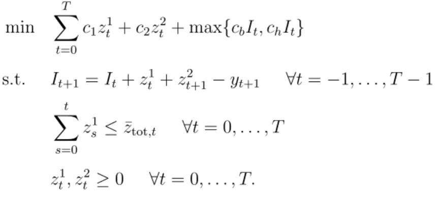
Consider a finite horizon, 𝑇 + 1 stage problem, in which the initial state, 𝑠0, is
known. We formulate the problem as follows: min 𝑧0∈𝑍0(𝑠0) 𝑔0(𝑧0) + E[ ˜𝑄1(𝑓0(𝑧0); 𝑌1))], (3.1) where ˜ 𝑄𝑡(𝑠𝑡; 𝑦𝑡) = min 𝑧𝑡∈𝑍𝑡(𝑠𝑡,𝑦𝑡) 𝑔𝑡(𝑧𝑡) + E[ ˜𝑄𝑡+1(𝑓𝑡(𝑧𝑡); 𝑌𝑡+1)]
for 𝑡 = 1, . . . , 𝑇 − 1, and ˜𝑄𝑇(𝑠𝑇; 𝑦𝑇) = min 𝑧𝑇∈𝑍𝑇(𝑠𝑇,𝑦𝑇)
𝑔𝑇(𝑧𝑇). The function ˜𝑄𝑡(𝑠𝑡; 𝑦𝑡)
is often called the value function or cost-to-go function. It represents the expected future cost that an optimal policy will incur, starting with a system in state 𝑠𝑡 with
realized uncertainty 𝑦𝑡. Of course, in practice it is impossible to solve this problem
because the distributions of 𝑌𝑡 are unknown. All that we know about the distribution
of 𝑌𝑡 comes from the available data.
A popular data-driven method for solving this problem is sample average approx-imation (SAA) [89]. In SAA, it is assumed that we have access to independent, iden-tically distributed (i.i.d.) training samples of 𝑌 , (𝑦1𝑖, . . . , 𝑦𝑇𝑖) for 𝑖 = 1, . . . , 𝑁 . The key idea of SAA is to replace the expectations over the unknown distributions of 𝑌 with empirical expectations. That is, we replace E[ ˜𝑄𝑇(𝑠𝑇; 𝑦𝑇)] with
1 𝑁 𝑁 ∑︀ 𝑖=1 ˜ 𝑄𝑇(𝑠𝑇; 𝑦𝑇𝑖).
With these known, finite distributions of the uncertain quantities, the problem can be solved exactly or approximately by various dynamic programming techniques. Addi-tionally, under certain conditions, the decisions obtained by solving the SAA problem are asymptotically optimal for (3.1) [86]. The basic SAA method does not incorpo-rate auxiliary data. In practice, this can be accounted for by training a generative, parametric model and applying SAA with samples from this model conditioned on the observed auxiliary data. However, this approach does not necessarily lead to asymptotically optimal decisions, so we instead focus on a variant of SAA that starts directly with the data.
3.1.2
Related Work
Multistage optimization under uncertainty has attracted significant interest from var-ious research communities. Bellman [6] studied these problems under the name dy-namic programming. For reference, see Bertsekas [11]. These problems quickly be-come intractable as the state and action space grow, with a few exceptions that admit closed form solutions, like linear quadratic control [46]. However, there exists a large body of literature on approximate solution methods (see, e.g., Powell [80]).
When the distribution of the uncertainties is unknown, but data is available, SAA is a common approach [87]. Alternative approaches include robust dynamic
programming [62] and distributionally robust multistage optimization [55]. Another alternative approach is adaptive, or adjustable, robust optimization (cf. Ben-Tal et al. [7], Bertsimas et al. [20]). In this approach, the later stage decisions are typically constrained to be affine or piecewise constant functions of past uncertainties, usually resulting in highly tractable formulations.
In the artificial intelligence community, reinforcement learning (RL) studies a sim-ilar problem in which an agent tries to learn an optimal policy by intelligently trying different actions (cf. Sutton and Barto [90]). RL methods typically work very well when the exact dynamics of the system are unknown. However, they struggle to in-corporate complex constraints that are common in OR problems. A vast literature also exists on bandit problems, which seek to find a series of decisions that balance exploration and exploitation (cf. Berry and Fristedt [10]). Of particular relevance is the contextual bandit problem (cf. Chapelle and Li [33], Chu et al. [38]), in which the agent has access to auxiliary data on the particular context in which it is operat-ing. These methods have been very effective in online advertising and recommender systems [70].
Recently, the single stage optimization problem with auxiliary data has attracted interest in the OR community. Ban and Rudin [3] studied a news-vendor problem in the presence of auxiliary data. Cohen et al. [40] used a contextual bandit approach in a dynamic pricing problem with auxiliary data. Ferreira et al. [49] used data on the sales of past products, along with auxiliary data about the products, to solve a price optimization problem for never before sold products. Bertsimas and Kallus [15] developed a framework for integrating predictive machine learning methods in a single-stage stochastic optimization problem. Recently, Ban et al. [4] developed a method to solve a multistage dynamic procurement problem with auxiliary data. They used linear or sparse linear regression to build a different scenario tree for each realization of auxiliary covariates. Their approach assumes the uncertainty is a linear function of the auxiliary covariates with additive noise. Our approach is more general because we do not assume a parametric form of the uncertainty.