Dealer Hoarding, Sales Push and Seed Returns: Characterizing the Interdependency between Dealer Incentives and Salesforce Management

MIT Sloan School Working Paper 4694-08

4/1/2008

Dealer Hoarding, Sales Push and Seed Returns: Characterizing the Interdependency between Dealer Incentives and

Salesforce Management

© 2008 Paulo Gonçalves

Paulo Gonçalves

All rights reserved. Short sections of text, not to exceed two paragraphs, may be quoted without

explicit permission, provided that full credit including © notice is given to the source.

Dealer Hoarding, Sales Push and Seed Returns:

Characterizing the Interdependency between Dealer

Incentives and Salesforce Management

Paulo Gonçalves

*

*

Paulo Gonçalves is a Visiting Assistant Professor at the MIT Sloan School of Management, 30

Wadsworth St. E53-339, Cambridge, MA, 02142. Phone (617) 253-3886. (Email: paulog@mit.edu). I am grateful to Karen Donohue and John Sterman for their valuable comments and insightful suggestions on earlier versions of the paper. I also thank the helpful comments from Hernan Awad, Joseph Johnson, Rogelio Oliva, Hazhir Rahmandad, Jeroen Struben, Stefan Wuyts and participants of the Behavioral Research in Operations Conference, the System Dynamics Winter camp, and the MIT Operations Management and System Dynamics Seminar.

Dealer Hoarding, Sales Push and Seed Returns:

Characterizing the Interdependency between Dealer Incentives and

Salesforce Management

Abstract

Hybrid seed suppliers experience excessive and costly rates of seed returns from dealers, who order in advance of grower demand realization and may return unsold seeds at the end of the season. Sales representatives know they must carefully gather information on grower demand for seed types and quantities to improve their demand forecast and better position their seeds. However, when pressured to

meet sales targets late in the sales cycle, salespeople abandon time-consuming seed positioning to push out dealers’ inflated orders. Such push effort leads to excessive returns, generating more inflated orders by dealers the following period and increasing the total sales that agents must achieve to meet their quota,

requiring them to push still more seed. Here we develop a formal dynamic model of the interaction of sales effort allocation and dealer hoarding behavior to understand the dynamics of corn seed returns through a model-based field study. Depending on the availability of sales resources, this biased sales effort allocation can generate a self-perpetuating stream of returns. While incentives to dealers solve the

dealer hoarding problem, they do not address pressured salespeople’s inadequate effort allocation to pushing seeds. Because decreased sales resources and overly-aggressive sales targets increase the pressure faced by salespeople, they also lead to higher seed returns. By understanding the causes of seed returns, our research informs us about the limitations of dealer incentives, shedding light on the important

roles of adequate sales resources management and of setting moderate sales targets.

Keywords: Salesforce management; sales resource allocation; dealer hoarding; dealer incentives; sales

1. Introduction

The hybrid seed industry experiences excessive and costly rates of seed returns (10% – 30%) from dealers. The demand for hybrid seeds such as corn is highly uncertain, heterogeneous, and deeply influenced by weather and current crop productivity. Year-to-year uncertainty in total corn planted area is high due to changes in prices and supplies (Westcott et al. 2003); planted area uncertainty by region and farm size is even higher. Hence, decisions about aggregate quantity to supply are difficult. Supply is also characterized by long product development and production delays. Suppliers offer hundreds of products, with several new seed hybrids each year. Short and unpredictable product lifecycles lead to rapid turnover of seed hybrids in the catalog. Decisions about what mix of corn-seed hybrids to produce are challenging and must occur months in advance of actual grower demand, leading to common short supply of specific hybrids. Due to uncertain demand and limited supply, dealers place their orders before grower demand is available and inflate them above demand expectations to hedge against shortages of possibly high performing hybrids. Dealer hoarding is a common feature of seed sales in the agribusiness industry.

Aware of dealer hoarding behavior, sales representatives gather information on grower demand for seed types and quantities to improve their demand forecast and better position their seeds. Such positioning effort improves sales forecasts and matches the supply of limited seed hybrids with uncertain demand, reducing seed returns this period. However, as the pressure to meet sales targets builds up late in the sales period, salespeople abandon time-consuming seed positioning to push out dealers’ inflated orders and quickly meet their sales targets. Pushing originally inflated orders that do not accurately match to grower demand leads to excessive returns this period. Clearly, the balance between the amounts of seeds positioned and pushed influences the total percentage of seeds returned this period. However, because salespeople must compensate for seed returned this period in the following one, seeds returned this period influence pressure on salespeople to meet sales targets in the next period. Hence, subsequent periods are interdependent. Sales returns in one period influences sales pressure and returns in future periods.

This research provides one example of an adaptation study (as defined by Gino and Pisano 2006) in behavioral operations management (Boudreau et al. 2003, Bendoly et al. 2006). In particular, we describe a field study and develop a formal mathematical model of the interaction of sales effort allocation and dealer hoarding behavior to understand the factors that contribute to the level of seed returns and how the dynamics of seed returns evolve over time. A descriptive field study based on semi-structured interviews and observations provided a number of potential hypotheses for the causes of the problem as well as a list of preferred courses of actions. Based on explicit assumptions elicited from the data and field study, we developed a prescriptive and structured dynamic theory represented in our mathematical model. In particular, we draw on our field work and interviews with managers at the supplier and dealers to develop the physical features (e.g., shipments, returns) of our model. On the behavioral side, we rely on research on cognitive psychology and human decision making (Hogarth 1987, Kahneman et al 1982, Plous 1993, Gersick 1988, Sterman 1989). To capture the interdependency and feedback processes between the physical and behavioral components, we rely on research on system dynamics (Forrester 1961, Morecroft 1985, Sterman 2000, Repenning 2001). Our research suggests that a key factor contributing to excessive seed returns is the unplanned allocation of sales resources to meet revenue quotas late in the sales cycle. In particular, we find that: (1) managerial pressure and sales representatives’ efforts to meet quotas coupled with dealer hoarding of scarce products can lead to high return rates, and (2) this mechanism is self-reinforcing.

Sales resource utilization plays a major role determining whether the system can present this self-reinforcing mechanism leading to a high-return equilibrium. Because salespeople must allocate effort between working hard (pushing seeds, i.e., improving performance by requesting dealers to take early delivery of seeds) and working smart (positioning seeds, i.e., generating a better forecast through information gathering on grower demand), a choice to allocate more effort to working hard is also a choice to allocate less effort to working smart. Task interdependence is particularly important when demand is highly uncertain and salespeople play a crucial role in generating better demand forecasts.

Since demand is highly uncertain in the agribusiness industry, pushing seeds contributes to excessive returns because it prevents salespeople from generating better forecasts through positioning.

While a traditional prescription to the problem described here would be to implement adequate incentives for dealers, our analysis shows that the effectiveness of dealer incentives depends on the adequacy of available sales resources. Our analysis shows that stronger penalties for dealer overordering reduce the fraction of returns (for a given salesforce size), however, a smaller salesforce increases the fraction of returns (for a given penalty level). Insufficient sales resources increase the pressure faced by salespeople tilting their time allocation toward pushing more seeds, which ultimately leads to more returns. While incentives to dealers solve the dealer over-ordering problem, they do not address pressured salespeople’s inadequate effort allocation to pushing seeds. Hence, both dealer incentives and sales resources must be managed together to ensure adequate system performance. Furthermore, because overly-aggressive sales targets also increase the pressure faced by salespeople, they too can lead to higher seed returns. By understanding the causes of returns, our research informs us about the limitations of dealer incentives, shedding light on the important roles of adequate sales resources management and of setting moderate sales targets.

The paper proceeds as follows. The next two sections present the literature review and describe the field study. Section 4 describes the main assumptions in the model. Section 5 develops a stylized model that captures the essential dynamics of returns in the seed supply chain. Section 6 shows the behavior of the model, proves that the system is characterized by multiple equilibria separated by a tipping point, and explores the interdependence between incentives and sales resources. We conclude with a discussion of our results, its implications, and opportunities for future research.

2. Literature Review

Two streams of literature are relevant to our work: the salesforce compensation and the product return policies literatures. Salesforce compensation schemes attempt to adequately reward salespeople for their efforts (Churchill, Ford and Walker 1981). Because monitoring salespeople’s effort is difficult and costly,

however, commissions are frequently used as a motivator due to its direct link between performance and financial rewards. Commissions, or incentive schemes, are widely used in sales environments to reward salespeople for their performance (Eisman 1993, Murphy and Sohi 1995). A number of papers shed light on the design of profit maximizing commission-only compensation schemes (e.g., Farley 1964, Weinberg 1975 and Srinivasan 198 1). While a commission-only scheme can inspire salespeople to work hard, it fails to engage salespeople in activities that are not linked to commissions (Basu et al. 1985, Cravens et al. 1993). Gonik (1978) suggests that good incentive schemes not only compensate salespeople for their effort, so as to motivate them to work hard, but also elicit “good and fresh field information on market potential for planning and control purposes.” A compensation scheme that combines a base salary with incentive pay (commissions) addresses the weakness of commission-only plans and accounts for approximately 73% of compensation plans used in practice (Peck 1982). These combined compensation schemes frequently pay commissions only if sales volume exceed a minimum sales threshold with commission levels progressing on a sliding scale until a maximum sales target. The salespeople in our field study received this type of compensation.

Much of the research on the use of sales quotas to motivate sales performance (Davis and Farley1971, Tapiero and Farley1975, Darmon 1979) is based on agency theory (Holmstrong 1979, Grossman and Hart 1983). In agency theory, a principal (firm) relies on an agent (salesperson) to act on the firm’s behalf but cannot observe the agent’s effort. Mantrala et al. (1994) and Mantrala et al. (1997) design incentive-compatible schemes where quotas can be effectively used to motivate salespeople. Two controlled experiments show that while higher quotas increase effort by salespeople (Winer 1973), sufficiently high quotas decrease effort (Chowdhury1993). Whereas such researchers focus on salespeople’s effort, Gaba and Kalra (1999) focus on riskiness to show that high quotas can induce salespeople to engage in high-risk behaviors.

Just like combined compensation schemes, product returns are also common in many different industries. Returns are frequently characterized as the cost of doing business, particularly in uncertain environments. Wood (2001) shows that lenient return policies increase product returns but also consumer

purchase probability, with a positive net sales effect. Pasternack (1985) shows it is suboptimal to offer a return policy giving retailers full credit for all unsold goods. Instead, a policy that offers partial refund for all returned goods can coordinate the supply chain in multi-retailer environments. A number of studies have investigated how to design adequate returns policies as well as control the level of returns (Padmanabhan and Png 1995, 1997; Pasternack 1985; Davis et al. 1995; Tsay 2001).

The literature on return policies also provides several examples of contracts that align retailer incentives with the manufacturers, leading to optimal supply chain profits (see Cachon 2003 for a review). Consider for instance contracts based on rebates. Webster and Weng (2000) find that a return policy that offers rebates for unsold goods at the end of the selling season encourages retailers to place larger orders and can increase manufacturer profits. However, when demand is lower than expected low profits can result from high rebate expenses. When retailer sales effort can influence customer demand, Taylor (2002) finds that a target rebate and returns contract, where the rebate is paid for each unit sold beyond a specified target threshold and unsold units can be returned, coordinates the supply chain. Ferguson, Guide and Souza (2006) propose a target rebate contract to induce the supply chain optimal amount of effort to reduce the number of false failure returns.

3. Field site

Our research rests on data gathered from a three-month in-depth study of a major U.S. supplier of hybrid corn and soybean seeds. Theoretical sampling (Glaser and Strauss 1967) was the motivation for site selection. The seed supplier faced excessive seed returns and provided an amazing opportunity for investigating its causes. Our research goals were twofold: to describe the dynamic behavior observed in the data and to develop theory that helped explain it and lead to improved performance. To develop our general theory of sales resource allocation, we followed standard methods for the development of grounded theory from case study research (Glaser and Strauss 1967, Eisenhardt 1989) and extended it with insights from the literature on judgment and decision making. Fisher (2007) describes a path to empirical research that is similar to the one we followed. Our starting point was descriptive and based on

semi-structured interviews and observations. This phase of the case study unearthed a number of potential hypotheses for the causes of the problem as well as a list of preferred courses of actions, all of which could be investigated later. The final product is a prescriptive and structured dynamic theory based on explicit assumptions elicited from the data.

Our field work included four site visits, weekly conference calls and approximately thirty semi-structured interviews with managers from the supplier and form dealers. Semi-semi-structured interviews allowed us to adapt to different contexts and individuals and to pursue new and unexpected cues suggested by early findings. Most interviewees (80%) were managers at the seed supplier working in different functional areas such as operations, logistics and supply chain management, quarterly initiatives, production planning, demand forecasting, sales and order processing. The remaining interviewees (20%) were managers working at dealers. We followed a joint collection, coding and analysis method for the case study. After site visits and specific interviews, we would revise recorded tapes, summarize field notes and follow up with clarifications or requests for further details. Model assumptions were grounded on the collected data and were verified regularly during weekly conference calls.

Two types of data were gathered and analyzed to ground the development of a system dynamics model of the problem: quantitative and qualitative data. Quantitative data indicated relationships that were initially not salient. For instance, the equation used for dealer hoarding was based both in an actual quote from a dealer, but was also incorporated in a spreadsheet file used by a manager at the seed supplier. Specific data on weekly seed requests by dealers and growers provided context on available information that dealers had when ordering from the supplier. Data on shipment rates, quarterly sales quotas, and fraction of such quotas met by salespeople at different times during the sales season permitted us to evaluate progression toward sales goals, evolving levels of sales pressure and also allowed us to verify the fit of our model behavior with that observed in the field study. Data on net sales and monthly returns could be cross checked against the other data. Qualitative data allowed us to understand the nature of

sales activities, the productivity and probability of returns associated with them, and also heuristics for effort allocation used by salespeople when facing sales pressure.

3.1. Problem description

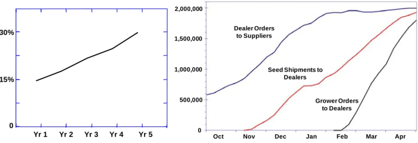
The major U.S. hybrid seed supplier that we studied experienced 30% of corn seed returns at the time of our intervention (Figure 1a). At that time, the direct costs (e.g., transportation, discards, obsolescence, retesting, reconditioning, repackaging) associated with corn returns at the field site reached 15% of net income. The indirect costs due to excess capacity were also large, since total production was 70% higher than net sales. Seed suppliers often produce in excess of sales and endorse some level of returns, encouraging dealers to overstock seeds to stimulate opportunistic sales or to limit competitors’ shelf space. While the benefits associated with additional sales do exist, the costs associated with excessive returns may, at times, far outweigh them.

2,000,000

1,000,000 1,500,000

500,000

Oct Nov Dec Jan Feb Mar Apr 0 Dealer Orders to Suppliers Seed Shipments to Dealers Grower Orders to Dealers

Figure 1. (a) Percent of corn-seed returns and (b) timing and volume of orders and shipments.

In the seed supply chain, the supplier sells seeds to dealers, who then resell them to growers. Grower demand for hybrid corn seeds is highly uncertain, heterogeneous, and deeply influenced by weather and current crop productivity. Growers place orders with dealers late in the sales season (at the beginning of the first quarter, Q1) and base their orders on hybrids that performed well in the current harvest (in the second half of the fourth quarter, Q4, of the previous year). Supply is characterized by long product development and production delays. Because corn-seed production decisions occur months in

0

Yr 1 Yr 2 Yr 3 Yr 4 Yr 5 30%

advance of grower demand, short supply of specific hybrids are common. Due to uncertain demand and limited supply, dealers place their orders before grower demand is available and inflate them above demand expectations to hedge against shortages of possibly high performing hybrids (Figure 1b). Shipments from the seed supplier to dealers also take place months in advance of demand.

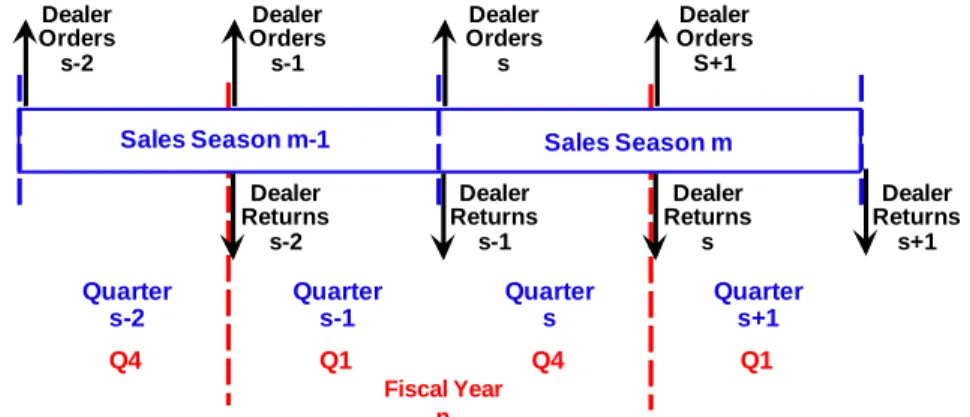
The seed supplier sales operations start at the beginning of the fourth quarter (Q4) and finish at the end of the first quarter (Q1) of every year. No dynamics contributing to sales or returns take place during Q2 and Q3; hence, these quarters are not modeled explicitly. Dealers place a large fraction of their orders at the beginning of the sales season (October) and returns occur at the end of the sales season (April). For computational convenience and simplicity, we account for orders as occurring at the beginning and returns at the end of each quarter. The quarterly orders and returns representation allows each quarter to be mathematically equivalent and can be interpreted as the fraction of orders and returns that have occurred in that quarter. Figure 2 provides an overview of the stylized seed sales process.

Dealer Orders s-2 Dealer Orders s-1 Dealer Orders s Dealer Orders S+1

Sales Season m-1 Sales Season m

Dealer Returns s-2 Quarter s-1 Quarter s Quarter s+1 Quarter s-2 Dealer Returns s-1 Dealer Returns s Dealer Returns s+1 Fiscal Year n Q1 Q4 Q1 Q4

Figure 2. Overview of seed sales process.

4. Model Assumptions

Five main assumptions are central to the dynamics of our model. The first describes the heuristic used by dealers to determine their order level. The second and third assumptions explain the productivity and probability of returns associated with sales activities available to salespeople. The fourth describes how sales pressure influences sales people effort allocation between different activities. The last assumption explains the sources of pressure that salespeople bear.

4.1. Dealer hoarding behavior

The first key assumption captures dealers’ hoarding behavior. Dealers place large orders early to hedge against the possibility of shortages. As one seed dealer expressed:

“We base our orders on last year’s sales and typically increase by 10-20% … [placing] 50% of total orders early in the season… We would order more than that, if we knew that supplies were short… If my sales rep would tell me that a certain variety is on short supply, I would order as much as I could, or as much as my rep would allow.”

Dealers’ initial orders are largely determined by the fraction of seeds returned the previous year. A large fraction of returns in one year leads to large expected returns in the following, causing dealers to inflate their orders to compensate for them. For instance, suppose a dealer orders the exact number of units to meet grower demand (G). Because of unpredictable weather conditions and imperfect knowledge of grower preferences, the dealer sells only a fraction of their order, (1-r)G, returning the rest (rG). The following quarter, to be able to sell G units and meet grower demand, dealers must order G/(1-r). For simplicity we assume that dealers have a good estimate of the underlying aggregate grower demand (G); poor estimates of grower demand would further amplify dealer hoarding and would strengthen the results reported here.

(

1

−

−1

)

=

S S

r

G

O

(1)

where rS-1 is the amount of returns, r, in the previous quarter, S-1.

4.2. Sales activities

During the sales season, salespeople must perform two (very different) types of tasks: position seeds with dealers or push seeds to them. Positioning means salespeople gather information on grower demand, before it is realized. Through field trips and interviews with growers and dealers, salespeople seek to understand which hybrids used in the previous season were high performing (similar hybrids will likely be in high demand this season); explore growers’ intentions to maintain planted areas or to rotate between crops; review the previous season’s hot selling hybrids; and survey dealers’ intentions to gain market share. Positioning seeds is a time intensive task. However, salespeople’s positioning effort leads to an

improved sales forecast, more effectively matching the supply with the highly heterogeneous demand. In contrast, pushing seeds to dealers does not improve the order forecast. Pushing seeds is comparatively quick and involves making phone calls to request dealers to take delivery of early inflated orders placed. By pushing seeds, salespeople increase their revenue contribution, rapidly closing the gap to their quarterly revenue targets.

4.2.1. Productivity of sales activities

While both activities consume the same resource, salespeople’s hours (H) averaging about 50 hours/week, our interviews with sales managers suggest that the time required to position (TA) a certain quantity of seeds is substantially higher than the time necessary to push (TB) the same amount. The time to position a load (L) of 40 bags of corn at dealers is on average 5 hours, whereas the time to push the same amount is on average 1 hour. Average times to position and push corn seeds were estimated using one year of seed shipment data and interviews with sales managers that identified periods where seeds were positioned or pushed. Assuming a constant number of salespeople in the workforce (W), we obtain the positioning rate (A) and pushing rate (B), in number of bags of corn/week, from the ratio of the total number of salespeople’s hours to the time to place (position or push) them at dealers.

A

T

L

H

W

A

=

⋅

⋅

and

B T L H W B= ⋅ ⋅

(2)

Since the time required to position (TA) is much greater than the time required to push (TB) the same amount of seeds, the positioning rate (A) is much slower than the pushing rate (B), i.e., because TA >> TB it follows that A << B.

4.2.2. Probability of returns due to sales activities

An important aspect of both sales activities is the impact they have on the probability of this period’s returns. Since salespeople’s positioning effort results in a better forecast of grower demand, it allows them to better align supply availability with specific dealers’ needs, thereby reducing the probability of returns. In contrast, since salespeople’s pushing effort results in shipping inflated dealers’ orders, it does

not align supply to demand leading to a higher probability of returns. We assume a fixed low probability of returns, PL, when salespeople position seeds and a high probability of returns, PL+PH, when salespeople push them. PL is the probability of returns that cannot be avoided by gathering demand information through positioning; and, PH is the probability of returns that can.

4.3. Sales effort allocation

The fourth assumption specifies the mechanism by which salespeople allocate their time between positioning and pushing seeds. First, for simplicity, we assume that salespeople do not shirk, so the total amount of salespeople’s hours available for positioning and pushing is fixed at 50 hours/week. While the goal-gradient hypothesis – originally proposed by Hull (1934) and recently revisited by Kivetz, Urminsky, and Zheng (2006) – suggests that proximity to the goal (deadline) leads to a stronger tendency to approach the goal (more salespeople’s hours/week), relaxing the fixed effort assumption would intensify the effectiveness of push efforts and strengthen the results presented here. The a fortiori assumption of fixed effort provides a more stringent test of our theory.

The formulation for salespeople’s allocation of effort between positioning and pushing seeds is based on our field study and also on research on motivation (Steel and König 2006) and work teams (Gersick 1988, Gersick and Hackman 1990). Our interviews suggest that salespeople initially devote time to positioning activities, but eventually they shift to pushing activities. According to a sales representative:

“We start out really trying to load toward true grower demand. Everybody makes an honest effort of positioning seeds. But when it gets down to crunch time … you are just shipping what you can get, where you can get it, and when you can get it.”

We aggregate salespeople, capturing their mean response over the distribution of possible response strengths. While the intensity of individual responses follow a distribution, our interviews suggest that salespeople respond similarly to the same stimuli. All salespeople interviewed characterized that they faced a “crunch time” during which they pushed seeds, expediting dealer orders. We implement the effort allocation shift from positioning to pushing activities as taking place when pressure to meet

revenues (p) is greater than a pressure threshold (pT). Combining the mechanism by which salespeople allocate effort between positioning and pushing activities and their associated return probabilities, we can determine the overall probability of returns. When sales pressure to meet quarterly goals (p) is below the threshold (pT), salespeople position seeds with the minimum unavoidable probability of returns (PL). When sales pressure exceeds the threshold (pT), salespeople push seeds with the maximum probability of returns (PL+PH ). The Overall Probability of Returns (PW) is:

(

)(

L H

)

L W P P P P =

α

+ 1−

α

+ and (3)

⎩

⎨

⎧

≥

<

=

T T

p

p

if

,

p

p

if

,

0

1

α

where α is the fraction of resources allocated to positioning seeds.

This formulation is supported by our field work which suggests, as illustrated by the quote above, that the switch from positioning to pushing takes place quickly. This sharp switch happens as salespeople realize that there are only few weeks left in the quarter to meet the revenue quota. This sharp reversal between activities is consistent with a number of theories of motivation (Steel and König 2006). Also, research on work teams (Gersick 1988, Gersick and Hackman 1990) suggests that the behavior of groups on tasks tends to shift to greater focus on completing the task about halfway through the time allotted. Similar results are obtained if the shift from positioning to pushing activities takes place linearly over time (for details see the derivation in Appendix 1).

4.4. Sales pressure

We model the pressure to meet quarterly revenue goals (p) as the fractional revenue required to meet the quota relative to the fraction amount of time remaining to do so. Specifically, the pressure is the ratio of the revenue gap fraction (RG) to the time remaining fraction (TG). The proposed pressure formulation leads to a pattern of behavior that is consistent with the explanations obtained from the value function of Prospect Theory (Kahneman and Tversky 1979) for empirical results in the goal literature on effort (Heath, Larrick and Wu 1999).

( )

_{( )}

( )

t TG t RG t p S S S = (4)

where quarters are discrete and characterized by the subscript S; time within a quarter is continuous and indexed by t; and, pS(t) is the pressure in quarter s at time t.

The fractional revenue gap measures the fraction of the original distance remaining to the revenue goal. Hanssens and Levien (1983) and Carroll et al. (1985) have used a similar construct to measure recruiter pressure in navy enlistment programs. More recently, Kivetz, Urminsky, and Zheng (2006) named it the goal-distance model and used it to describe the rate at which customers allocate effort as a function of the fractional distance remaining to the goal. Here, the fractional revenue gap (RG) is modeled as the difference between the target revenue (R*) plus lost revenues from previous quarter returns (RLS-1) and current accumulated gross revenues (GRS), normalized by the target revenue (R*) and last quarter lost revenues (RLS-1). That is, to meet the quota this period the salesperson must achieve revenues of R* plus enough revenues to cover the cost of returns from last period.

( )

(

₍

)

₎

( )

1 * 1 * − −

+

−

+

=

S S S S S S

RL

R

t

GR

RL

R

t

RG

(5)

While the time remaining to make a decision is not traditionally incorporated in many marketing models, research applying regret theory to model the impact of coupon expiration date on consumer behavior suggests that high redemption rates take place just prior to the expiration date (Inman and McAlister 1994). In addition, time remaining is a major component of hyperbolic discounting theory, a theory that helps to describe choice behavior over time (Ainsle and Haslam 1992). The fractional time remaining in the quarter (TG) is given by the ratio of the time remaining to the total time available in the quarter, T (13 weeks), where the time remaining is given by the total time in the quarter (T) minus the time elapsed (t).

( )

T t T t TG_S = − (6)

As time to meet revenue quotas elapses, the fractional time remaining approaches zero and salespeople pressure rocket toward infinitum. It is possible to improve on the formulation above by adding a constant, τ, characterizing the minimum fractional time required to complete the simplest task. This more robust formulation is consistent with Mazur (1987), but unnecessary here. In our hybrid discrete-quarters continuous-time model, model parameters are reinitialized at the beginning/end of each quarter and the maximum sales pressure is inversely proportional to the time step of integration.

5. Model Structure

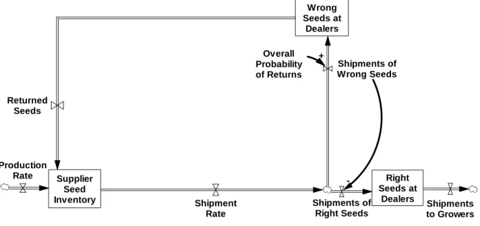
Figure 3 provides a more detailed view of the central structure in a system dynamics model of the corn-seed supply chain. Stocks, represented by rectangles, correspond to accumulations of corn-seeds. Stocks are mathematically equivalent to integrals. Flows, represented by arrows with valve symbols, correspond to actions, such as shipments. Flows are mathematically equivalent to derivatives. Solid arrows capture the influence of other variables on the flows.

Supplier Seed Inventory Production Rate Shipment Rate Wrong Seeds at Dealers Right Seeds at Dealers Shipments of Right Seeds Shipments of Wrong Seeds Returned Seeds Overall Probability of Returns + Shipments to Growers

-Figure 3. Stock-and-flow diagram for seed supplier shipments.

At the beginning of each quarter, the Production Rate and Returned Seeds from the previous quarter replenish the stock of Seed Supplier Inventory. Sales effort to position or push seeds determines

the Shipment Rate, according to the positioning and pushing rates given by equation 2. Shipments decrease the supplier inventory. The probability of having the “right” (or “wrong”) seeds, i.e., seeds with (or without) corresponding grower demand, reaching dealers follows equation (3) and depends on sales effort allocation to positioning or pushing seeds. The quantity of Wrong Seeds at Dealers accumulates over the quarter at a rate given by the product of the Shipment Rate and the Overall Probability of Returns (PW). Wrong seeds accumulated at dealers return to the supplier inventory at the end of the quarter and are accounted as Lost Revenues from Returns. The quantity of Right Seeds at Dealers accumulates over the quarter at a rate given by the Shipment Rate minus Shipments of Wrong Seeds. Right seeds accumulated at dealers are shipped to growers.

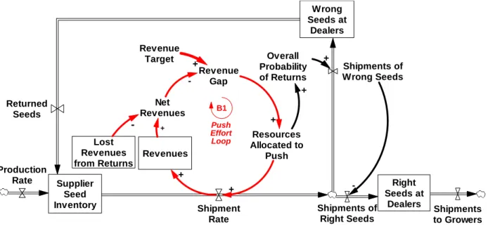
Supplier Seed Inventory Production Rate Shipment Rate Wrong Seeds at Dealers Right Seeds at Dealers Shipments of Right Seeds Shipments of Wrong Seeds Returned Seeds Overall Probability of Returns + Lost Revenues from Returns Net Revenues Revenues Revenue Gap -+ -+ Resources Allocated to Push + + B1 Push Effort Loop + Revenue Target + -Shipments to Growers

Figure 4. Push effort balancing feedback loop.

Figure 4 incorporates an important feedback loop capturing salespeople’s heuristic for pushing seeds. The push effort loop (B1) is a balancing (or negative) feedback mechanism that regulates the revenue gap by adjusting the amount of effort allocated to pushing seeds. A large discrepancy (Revenue

Gap) between the Revenue Target and Net Revenues leads to high pressure to meet quarterly revenue

goals. While sales pressure is below the threshold, salespeople allocate resources to positioning seeds, shipping seeds to dealers with the positioning rate, A, and a probability of shipping wrong seeds, PL.

However, once sales pressure rises above the threshold, salespeople start pushing seeds, shipping seeds to dealers with the faster pushing rate, B, and a higher probability of shipping wrong seeds, PL+PH. As salespeople push seeds, they accumulate Revenues more rapidly in the quarter, closing the revenue gap and easing the pressure to meet quarterly revenue quotas.

Supplier Seed Inventory Production Rate Shipment Rate Wrong Seeds at Dealers Right Seeds at Dealers Shipments of Right Seeds Shipments of Wrong Seeds Returned Seeds Overall Probability of Returns + Lost Revenues from Returns Net Revenues Revenues Revenue Gap -+ + -+ Resources Allocated to Push + + B1 Push Effort Loop R1 Returns Loop + Revenue Target Delay + -Shipments to Growers

Figure 5. Returns reinforcing feedback loop.

Figure 5 incorporates a reinforcing (or positive) feedback mechanism, the returns loop (R1), capturing the impact of seed returns in the system. The reinforcing loop can operate in a vicious or virtuous way. If sales resources are sufficient to position a large quantity of seeds, pressure to meet revenue goals remains below the pressure threshold for most of the quarter, resulting in a small amount of seeds pushed and consequently a small amount of returns. The following quarter, dealers do not need to inflate orders as much and sales resource requirements are even lower, requiring salespeople to push an even smaller amount of seeds, leading to even lower returns. As described here, the reinforcing loop behaves in a virtuous way. In contrast, if sales resources are insufficient to position a sufficiently large quantity of seeds, pressure to meet revenues goals will mount. After pressure increases above the threshold, salespeople will push more seeds, leading to a higher probability of shipping seeds to dealers with inadequate grower demand and resulting into a large fraction of returns. Higher returns result in lost

revenues; increase the following quarter’s revenue gap and the pressure on salespeople; and raise resource requirements for the following quarter, compelling salespeople to push even more seeds. The loop works in a vicious way, leading to high returns and poor salesforce performance.

Perfectly rational salespeople (or firm managers) would not allow such a vicious cycle to occur. But properly assessing the costs and benefits of pushing and seeing how pushing today hurts revenue tomorrow is difficult. The benefits of pushing seeds are recognized immediately – salespeople get rewarded (they receive a cash bonus) for meeting the quarterly revenue target, but the costs associated with returns occur only much later. Also, while the benefits of pushing seeds are financial, the costs of returns to salespeople are not. When returns occur at the end of the quarter, the associated lost revenues are accounted for in the following quarter, increasing the revenue gap, raising pressure to meet the quarterly goals and compelling salespeople to push even more seeds.

6. Model Behavior and Analysis

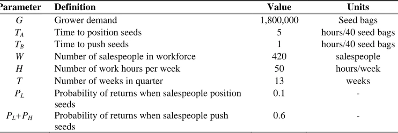
Table 1 presents the base case parameters for the model. Since the important activity with respect to seed sales occur in the first and fourth quarters, our model, without loss of generality, captures two quarters in each simulated year (Q4 and Q1). Base case results are shown in Figures 6 and 7. Without an exogenous (external) shock, system behavior in the base case scenario is the same in each quarter. To explore the internal dynamics of the modeled system, we study its operation without external random shocks; instead exploring how a single perturbation may trigger an endogenous increase in returns. We discard the first five years of each simulation to avoid initial transient behavior.

TABLE 1–BASE CASE PARAMETERS

Parameter Definition Value Units

G Grower demand 1,800,000 Seed bags

TA Time to position seeds 5 hours/40 seed bags

TB Time to push seeds 1 hours/40 seed bags

W Number of salespeople in workforce 420 salespeople

H Number of work hours per week 50 hours/week

T Number of weeks in quarter 13 weeks

PL Probability of returns when salespeople position seeds

0.1 -

PL+PH Probability of returns when salespeople push seeds

0.6 - Note: Base case parameters are motivated by values obtained through interviews with the seed supplier. Parameter values for PL and PH are difficult to assess for the real supplier. Here, their choice is arbitrary. The behavior of the system would be similar for a large range of values (e.g., higher PL and lower PH).

6.1. Base case

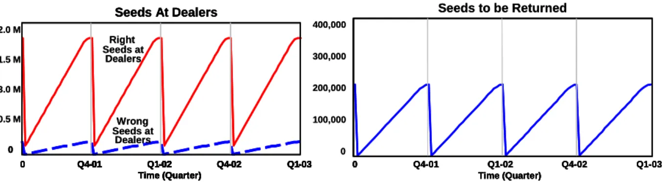
Early in the quarter salespeople have plenty of time to sell, pressure to meet the revenue target is low (Figure 6a) and salespeople allocate effort to positioning seeds (Figure 6b). Shipments to dealers take place at the positioning rate, A. Since the probability of shipping seeds without corresponding grower demand is small, PL, the amount of “right” seeds at dealers, increases rapidly (Figure 7a). If sales resources are insufficient to position all seeds and meet the revenue targets, pressure increases as the end of the quarter approaches (Figure 6a).

Sales Pressure 3.0 1.5 0 0 Q4-01 Q1-02 Q4-02 Q1-03 Time (Quarter) Pressure Threshold 0 Q4-01 Q1-02 Q4-02 Q1-03 Time (Quarter) - - - -Sales Pressure Sales Pressure 3.0 1.5 0 0 Q4-01 Q1-02 Q4-02 Q1-03 Time (Quarter) Pressure Threshold 0 Q4-01 Q1-02 Q4-02 Q1-03 Time (Quarter) - - - -Resource Allocation 28,000 21,000 14,000 7,000 0 Resources Allocated to Position Resources Allocated to Push 0 Q4-01 Q1-02 Q4-02 Q1-03 Time (Quarter) 0 Q4-01 Q1-02 Q4-02 Q1-03 Time (Quarter) - - - -Resource Allocation 28,000 21,000 14,000 7,000 0 Resources Allocated to Position Resources Allocated to Push Resources Allocated to Push 0 Q4-01 Q1-02 Q4-02 Q1-03 Time (Quarter) 0 Q4-01 Q1-02 Q4-02 Q1-03 Time (Quarter) - - - -Sales Pressure

Figure 6. (a) Sales pressure and (b) resource allocation.

When the pressure reaches a threshold, salespeople shift resource allocation from positioning to pushing seeds (Figure 6b). During these high-pressure “crunch” periods, seed shipments take place at the much faster pushing rate, B, and the higher probability of returns, PL+PH (Figure 7a). The increased

shipment of wrong seeds accumulates over time, leading to higher returns to the seed supplier at the end of the quarter (Figure 7b).

Seeds At Dealers 2.0 M 1.5 M 3.0 M 0.5 M 0 Seeds at Right Dealers Seeds at Wrong Dealers 0 Q4-01 Q1-02 Q4-02 Q1-03 Time (Quarter) 0 Q4-01 Q1-02 Q4-02 Q1-03 Time (Quarter) -01 02 - -Seeds At Dealers 0 0 Q4-01 Q1-02 Q4-02 Q1-03 Time (Quarter) 0 Q4-01 Q1-02 Q4-02 Q1-03 Time (Quarter) -01 02 - -Seeds At Dealers 2.0 M 1.5 M 3.0 M 0.5 M 0 Seeds at Right Dealers Seeds at Wrong Dealers 0 Q4-01 Q1-02 Q4-02 Q1-03 Time (Quarter) 0 Q4-01 Q1-02 Q4-02 Q1-03 Time (Quarter) -01 02 - -Seeds At Dealers 0 0 Q4-01 Q1-02 Q4-02 Q1-03 Time (Quarter) 0 Q4-01 Q1-02 Q4-02 Q1-03 Time (Quarter) -01 02 - -Seeds to be Returned 400,000 300,000 200,000 100,000 0 0 Q4-01 Q1-02 Q4-02 Q1-03 Time (Quarter) 0 Q4-01 Q1-02 Q4-02 Q1-03 Time (Quarter) - - - -Seeds to be Returned 400,000 300,000 200,000 100,000 0 0 Q4-01 Q1-02 Q4-02 Q1-03 Time (Quarter) 0 Q4-01 Q1-02 Q4-02 Q1-03 Time (Quarter) - - -

-Figure 7. (a) Seed stocks at different dealers and (b) shipments to wrong dealers.

In the base case, the simulated supplier allocates most resources to positioning seeds, and pushes only a modest amount of wrong seeds to dealers, so total returns are relatively small. While dealers’ orders in the following quarter compensate for the fraction of seeds returned in the previous one, the small amount of returns allows salespeople to allocate most of their time to positioning seeds, thereby limiting future returns. Contrasting the base case behavior with observations from the field study, we note that seed stocks accumulated at regional dealers follow closely the pattern in the model. However, sales pressure increases earlier in the quarter, a significant amount of sales effort is devoted to pushing seeds, and the fraction of returns is considerably higher.

6.2. Demand shocks

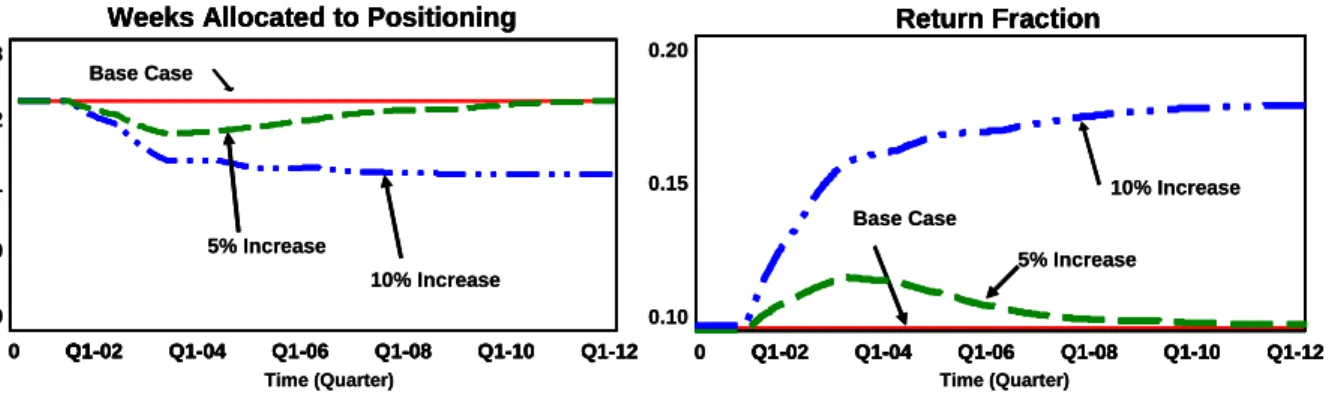
Given the desired mode of operation in the base case, it is important to explore whether the modeled system can generate the excessive returns observed in the seed supplier as well as what factors may contribute to it. Two simulation experiments provide insight into these questions. In these simulations, we temporarily increase grower demand (and sales quotas) in the first quarter, by 5 percent and 10 percent respectively, returning them to base case levels during the remaining quarters. This transient increase in demand might arise due to a rise in the price growers can get for their corn or an increase in government subsidies.

With fixed sales resources and increased dealer orders, salespeople are unable to position all seeds and must increase their dependence on pushing seeds to dealers. In both simulations, following the increase in grower demand, the fraction of time salespeople allocate to positioning falls (Figure 8a). As more seeds are pushed, the probability of sending the wrong seeds increases, leading to more returns (Figure 8b). In the case of the 5% increase, the fraction of time allocated to positioning begins to recover and the fraction of seeds returned falls after a while. Though the demand shock increases the fraction of returns temporarily, the system is able to recover and goes back to the desired operation mode where salespeople position their seeds most of the time.

Weeks Allocated to Positioning 13 11 9 10% Increase Base Case 5% Increase

Weeks Allocated to Positioning

12

10

0 Q1-02Q1- Q1-04- Q1-06- Q1-08- Q1-10- Q1 12

-Time (Quarter)

Weeks Allocated to Positioning 13 11 9 10% Increase Base Case 5% Increase

Weeks Allocated to Positioning

12 10 0 Q1-02Q1- Q1-04- Q1-06- Q1-08- Q1-10- Q1 12 -0 Q1-Q1-02Q1-Q1-02 Q1-04Q1-04-- Q1-06Q1-06-- Q1-08Q1-08-- Q1-10Q1-10-- Q1 12Q1 12- -Time (Quarter) Return Fraction 0.20 0.15 0.10 10% Increase Base Case 5% Increase Return Fraction 0 Q1-02Q1- Q1-04- Q1-06- Q1-08- Q1-10- Q1 12 -Time (Quarter) Return Fraction 0.20 0.15 0.10 10% Increase Base Case 5% Increase Return Fraction 0 Q1-02Q1- Q1-04- Q1-06- Q1-08- Q1-10- Q1 12 -0 Q1-Q1-02Q1-Q1-02 Q1-04Q1-04-- Q1-06Q1-06-- Q1-08Q1-08-- Q1-10Q1-10-- Q1 12Q1 12- -Time (Quarter)

Figure 8. (a) Weeks allocated to positioning and (b) return fraction.

The behavior resulting from a 10% increase in demand, however, is quite different. Here, the fraction of time allocated to positioning does not recover after grower demand returns to normal levels. As more seeds are pushed to dealers, a larger fraction is returned, requiring even more pushing the following quarter. Following the transient increase in demand, the system settles in a new operation mode, in which a large fraction of salespeople’s effort is allocated to pushing seeds and the fraction of seeds returned is permanently high. In this case, the demand shock is sufficient to bring the system to a high-return operation mode.

6.3. Phase plot analysis

To understand why different size shocks generate such divergent behavior, we follow an analysis procedure developed by Repenning (2001). First, we reduce the high order nonlinear structure of the

system to a one-dimensional map, by studying the system dynamics between quarters. Since dealer orders in a quarter depend on seeds returned in the previous quarter, and since the system is integrable, we can capture the dynamics of returns as a discrete time map in which returns this quarter, r S, are a function of returns last quarter, rS-1, that is, rS = f(r S-1); see, e.g., Ott (1993). Second, we use the map to characterize the conditions required for the different operating modes of the system to emerge. Resource availability and the positioning and pushing rates in the sales organization play an important role in determining the operating mode of the system. To derive the map, we begin with the determination of returns as a function of salesforce effort (see appendix 1 for details on this derivation):

(

)

(

)

⎟⎟

_⎠

⎞

⎜⎜

⎝

⎛

−

+

−

+

=

C F C C F H L S

t

T

B

At

t

T

B

Max

P

P

r

0

,

(7)

where A is the positioning rate, B is the pushing rate, tC is the critical time when salespeople shift from positioning to pushing (associated with the pressure threshold, pT), and TF is the time that shipments end (which may occur before the end of the quarter, T.) If TF=T, the supplier may or may not be able to ship

all dealer orders. Note that pushing seeds has the positive effect of allowing the supplier to ship a greater fraction of dealer orders. The additional amount of seeds that can be shipped while pushing is given by . However, pushing has the negative impact of leading to a higher probability of returns. In particular, pushing leads to returns of

(

B

−

A

)(

T

F

−

t

C

)

(

)

[

B

P

L

+

P

H

−

AP

L

]

(

T

F

−

t

C

)

. For the parameter values established in table 1 (TA=5, TB=1, PL=0.1, PH=0.5), the positive effect of shipping more seeds is higher (by almost 50%) than the negative impact of returns. Therefore, we make an a priori assumption that the net impact of pushing is advantageous to the company.

The equation for the return fraction (7) has an intuitive interpretation. The minimum return fraction, PL, takes place when the critical time to switch from positioning to pushing is sufficiently high ( ). When rS = PL, salespeople only position seeds and never push. The maximum return fraction, PL +PH, occurs when tC equals zero (tC = 0). If the critical time to switch to pushing is zero, salespeople will push seeds from the beginning of the quarter and returns will be given by the maximum

T t T_F ≤ _C ≤

probability of shipping wrong seeds (PL +PH). Between these extreme conditions, the degree of excess returns, PH, is given by:

(

)

(

)

⎟⎟

_⎠

⎞

⎜⎜

⎝

⎛

−

+

−

C F C C F

t

T

B

At

t

T

B

(8)

Since the numerator in equation (8) provides the total amount of seeds pushed to dealers and the denominator gives the total amounts of seeds shipped, the ratio suggests that the degree of excess returns is proportional to the fraction of seeds pushed to dealers. Moreover, it is possible to characterize the critical time (tC) from the definition of pressure in equation (3) and after we introduce tC in the equation above, the return fraction can be expressed as (see appendix 2 for details on this derivation):

(

)

(

)

(

)

⎟

⎟

⎟

⎟

⎠

⎞

⎜

⎜

⎜

⎜

⎝

⎛

⎟

⎟

⎟

⎟

⎠

⎞

⎜

⎜

⎜

⎜

⎝

⎛

−

+

−

−

⋅

−

−

⋅

+

=

− − −

T

T

r

r

G

AT

p

p

Min

r

G

A

Max

P

P

r

S S T T S H L S

,

1

1

1

1

1

,

0

1 1 1 (9)

This equation captures the dynamics of product returns in a multi-activity sales environment system by relating the fraction of seeds returned in a quarter, rS, to the amount of seeds that can be positioned in a quarter (AT), the quarterly grower demand (G), the pressure threshold for pushing (pT) and the return fraction in the previous quarter rS-1. A phase plot relating the current return fraction, rS, to the previous quarter return fraction, rS-1, provides a graphical representation of the return map in equation (9). Repenning (2001) provides an interesting application of an analogous phase plot to understand the emergence and persistence of fire-fighting in multi-product development systems.

L

0 0.2 0.4 0.6 0.8 0 0.2 0.4 0.6 0.8 1 r r

M

H

1 S-1 S

Figure 9. Phase plot for return fraction.

Note: Solid circles (fixed points) represent equilibria. The return fraction in the low (L) and high (H) equilibria are stable – once reached the system will remain there. The middle (M) equilibrium is unstable. A system starting close to (M) will follow the arrows toward one of the two stable equilibria.

To interpret the dynamics represented by the phase plot, shown in figure 9, start with a point in the x-axis, referring to the return fraction in the previous quarter, rS-1, and through the phase function find the associated value on the y-axis, the current return fraction, rS. To find the return fraction in the next quarter, rS+1, start with the value obtained for rS on the x-axis. Repeating the process allows us to obtain a summary of the evolution of the return fraction in the system. Note that any time the phase plot crosses the forty five degree line, the return fraction in the previous quarter will equal the current return fraction (rS = rS-1). Since the system is a one-dimensional map, these are the fixed points where the system is in equilibrium. Fixed points where the phase plot has a slope less than 1 are stable (e.g., the low (L) and high (H) equilibria.) Balancing feedbacks dominate the dynamics of the system such that departures from equilibrium are counteracted. Once these fixed points are reached, the system will remain there. In contrast, fixed points where the phase plot has a slope greater than 1 are unstable (e.g., the middle (M) equilibrium). Positive feedbacks dominate the dynamics around unstable equilibria; departures from these fixed points are reinforced, following the trajectory indicated by the arrows on the phase plot. Hence, if the system starts with a return fraction (rS-1) below the unstable equilibrium, the positive loop will operate in a virtuous way moving the system toward the equilibrium with a low return fraction (L). If instead, the system starts with a return fraction (rS-1) above the unstable equilibrium, the positive loop will operate in a

vicious way moving the system toward the equilibrium with a high return fraction (H). The unstable

equilibrium, or tipping point, determines the position where the positive returns loop changes direction, or

tips, from a virtuous operation mode to a vicious one, and vice-versa.

There are important implications of these insights. First, the existence of an unstable equilibrium that allows for a tipping point suggests that even when the system starts in the desired operation mode, there is no guarantee that it will remain there. This insight explains the difference in the dynamic behavior observed in the two simulation experiments above. In the base case, the system operates in a desired operation mode with a low return fraction. While the five percent increase in grower demand leads to a higher return fraction in the current year, it is insufficient to push the system beyond the tipping point, so the system returns to the original equilibrium. However, the ten percent increase in grower demand is large enough to push the system beyond the unstable equilibrium, taking the system to the equilibrium with high return fraction. Finally, the existence of the stable equilibrium with high returns (rS= PL+PH) suggests that the problem of high returns can be a steady-state phenomenon to seed suppliers.

6.4. Characterizing possible system phase plots

The analysis above provides an explanation of how a sufficiently large shock can push the system beyond the tipping point, leading to an undesired mode of operation with a high return fraction. Here, we characterize the conditions under which the unstable equilibrium arises in the system. The conditions that contribute to the existence of a tipping point are obtained through analysis of equation (9). When the maximum constraint binds at zero, the equilibrium return fraction is simply rS = PL, indicating that a single equilibrium with low returns exists. To analyze which conditions allow the maximum constraint to bind at zero, we must first look at the minimum constrain. The minimum constraint will bind at the value of T, only if the number of seeds that can be positioned in the quarter (AT) is larger than the total seeds that the supplier must ship out

(

G

(

1

+

r

_S−1

) (

1

−

r

_S−1

)

)

, consisting of the sum total dealer orders

(

)

(

G

1

−

r

_S−1

)

and the amount of prior-quarter returns

(

Gr

_S−1

(

1

−

r

_S−1

)

)

. When the condition above holds, salespeople’s choice of the pressure threshold (pT) does not matter and the maximum constraint binds if

the number of seeds that can be positioned in the quarter (AT) is larger than total dealer orders

(

)

(

G

1

−

r

S−1

)

))

. Since the latter follows from the requirements for the minimum constraint to bind, we find that salespeople must have sufficient resources to position all desired shipments to dealers, regardless of the previous quarter returns

(

)

. In the worst case scenario, the fraction of previous quarter returns

would equal (PL+PH). Figure 10 shows the phase plot for the single equilibrium at = PL when

1 − S

r

(

S

r

(

)

(

P

L

P

H

)

(

P

L

+

P

H

G

AT

>

1

+

+

1

−

. Intuitively, if sales resources are sufficient to enable all seeds to be positioned at all times no matter how high returns are, the system will always recover to a high performance equilibrium with the low return rate. Such a situation is highly unlikely, as the salesforce needed and the resulting costs would be prohibitive. A firm finding itself with so much sales capacity would almost surely downsize the sales organization to eliminate the excess capacity.

In contrast, when the positioning capacity (AT) is close to zero, which can happen if the time to position seeds (TA) is extremely high, or the salesforce is so small that salespeople never position seeds, then the equilibrium return fraction is simply ≅ PL+PH. (The phase plot associated with this equilibrium is not shown.) Because salespeople have insufficient resources to position any seeds, they must push all of them to dealers. This high equilibrium return fraction = PL+PH is equivalent to the one obtained if the pressure threshold for pushing (pT) is one (equivalent to a critical time, tC, equal to zero). Intuitively, when there are so few resources relative to the workload requiring salespeople to push all the time, the system will always evolve to the high-return equilibrium even if demand temporarily falls. Firms would normally not reduce their salesforce capacity so much relative to the workload, forcing the sales system to always be in push mode. We therefore expect that this extreme condition is also likely to be rare (if for no other reason than that such a firm will have an uncompetitive rate of returns and either add sales resources or go out of business).

S

r

S

Three other general cases for the phase plots remain. Since in equilibrium , we solve for the fixed points by substituting for in equation (9), yielding a quadratic equation in .The equilibrium values of are given by the roots of:

1 −

=

S S

r

r

S

r

r

S−1

r

S S

r

(10)

0

2

+

+

=

c

br

ar

_{S S} where:

a

=

p

_T

G

+

AT

(

1

−

P

_H

(

p

_T

−

1

)

)

(

)

(

L H

)

(

(

L H

)

)

T

G

P

P

AT

P

P

p

b

=

1

+

+

−

1

−

+

(

+

)

−

(

(

+

)

+

(

−

1

)

)

=

p

_T

G

P

_L

P

_H

AT

P

_L

P

_H

P

_H

p

_T

c

The roots are: r_S

(

b b2 4ac

)

2a

(

b

)

2a 2

,

1 = − ± − = − ±Δ

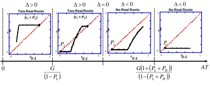
Depending on the seed positioning capacity (AT), grower demand (G), the pressure threshold for pushing (pT), and the probabilities (PL, PH), equation (10) may have zero roots (if Δ < 0), one root (if Δ = 0), or two real roots (if Δ > 0), equivalently generating the same number of equilibria. Figure 10 shows

these three general cases (and the previously mentioned case of a single low return equilibrium) as a function of the company’s available resources for positioning seeds (AT). As the diagram suggests, as the company increases positioning capacity (AT) the shape of the phase plot changes from a system with a single low performance equilibrium (at PL+PH), to one with three equilibria – two stable (one low-return at PL and one high-return) and one unstable – and then to one with a single high performance equilibrium (at PL). (Note that the phase plot case with Δ = 0 is not shown.)

r r r r L

P

r r L

P

0

>

Δ

0

>

Δ

Δ

<

0

Two Real Roots (r1< PL)

Two Real Roots (r1> PL) No Real Roots

AT

(

)

(

)

(

)

(

L H

)

H L

P

P

P

P

G

+

−

+

+

1

1

r r L

P

1 1 0 0 1 1 0 0 1 1 0 0 1 1 0 0

0

=

Δ

(

P

L

)

G

−

1

0

0

<

Δ

No Real Roots S-1 S S-1 S-1 S-1 S S S

Figure 10. The system’s phase plots.

The first case occurs when the supplier has insufficient resources to position the lowest possible amount of seeds demanded by dealers

(

AT

<

G

(

1

−

P

_L

)

)

. Here, the quadratic equation has two real roots (Δ>0) but one of them lies below the minimum return fraction (rS1 < PL). This situation can arise for different values of the pressure threshold for pushing (pT). Here, the system has a single stable low-performance equilibrium with a high probability of returns and the positive loop of returns always works as a vicious cycle. Returns will be high but lower than PL+PH, because that can only be achieved if no seeds are positioned in the quarter. The second case arises when the supplier has sufficient resources to position the lowest possible amount of seeds demanded by dealers,

(

AT

>

G

(

1

−

P

_L

)

)

, insufficient resources to position the maximum amount of seeds required by dealers,

(

)

(

P

L

P

H

)

(

(

P

L

P

H

))

G

AT

<

1

+

+

1

−

+

, and the quadratic equation has no real roots (Δ<0). This

situation arises when the pressure threshold (pT) is high, allowing salespeople to use the available resources to position seeds. Here, the system has a single stable equilibrium at the low probability of returns (rS=PL), determined by the maximum function in equation 9 and not by the roots of the quadratic equation. In this situation, the positive loop of returns always works as a virtuous cycle. The final case arises when the supplier has sufficient resources to position the lowest possible amount of seeds demanded by dealers,

(

AT

>

G

(

1

−

P

_L

)

)

, insufficient resources to position the maximum amount of