Protein secondary structure assignment revisited: a detailed analysis of different assignment methods.

HAL Id: inserm-00090199

https://www.hal.inserm.fr/inserm-00090199

Submitted on 29 Aug 2006

HAL is a multi-disciplinary open access

archive for the deposit and dissemination of

sci-entific research documents, whether they are

pub-lished or not. The documents may come from

teaching and research institutions in France or

abroad, or from public or private research centers.

L’archive ouverte pluridisciplinaire HAL, est

destinée au dépôt et à la diffusion de documents

scientifiques de niveau recherche, publiés ou non,

émanant des établissements d’enseignement et de

recherche français ou étrangers, des laboratoires

publics ou privés.

detailed analysis of different assignment methods.

Juliette Martin, Guillaume Letellier, Antoine Marin, Jean-François Taly,

Alexandre de Brevern, Jean-François Gibrat

To cite this version:

Juliette Martin, Guillaume Letellier, Antoine Marin, Jean-François Taly, Alexandre de Brevern, et

al.. Protein secondary structure assignment revisited: a detailed analysis of different assignment

methods.. BMC Structural Biology, BioMed Central, 2005, 5 (17), pp.17. �10.1186/1472-6807-5-17�.

�inserm-00090199�

Open Access

Research article

Protein secondary structure assignment revisited: a detailed

analysis of different assignment methods

Juliette Martin*

_{, Guillaume Letellier}

_{, Antoine Marin}

_{, Jean-François Taly}

_,

Alexandre G de Brevern

_{and Jean-François Gibrat}

Address: 1_{INRA, Unité Mathématiques Informatique et Génome, Domaine de Vilvert, 78352 Jouy en Josas Cedex, France and} 2_{INSERM U726,} Equipe de Bioinformatique Génomique et Moléculaire, Université Paris 7, case 7113, 2 place Jussieu, 75251 Paris cedex 05, France

Email: Juliette Martin* - juliette.martin@jouy.inra.fr; Guillaume Letellier - guillaume.letellier@jouy.inra.fr; Antoine Marin - antoine.marin@jouy.inra.fr; Jean-François Taly - jean-francois.taly@jouy.inra.fr; Alexandre G de Brevern - debrevern@ebgm.jussieu.fr; Jean-François Gibrat - jean-francois.gibrat@jouy.inra.fr

* Corresponding author

Abstract

Background: A number of methods are now available to perform automatic assignment of

periodic secondary structures from atomic coordinates, based on different characteristics of the secondary structures. In general these methods exhibit a broad consensus as to the location of most helix and strand core segments in protein structures. However the termini of the segments are often ill-defined and it is difficult to decide unambiguously which residues at the edge of the segments have to be included. In addition, there is a "twilight zone" where secondary structure segments depart significantly from the idealized models of Pauling and Corey. For these segments, one has to decide whether the observed structural variations are merely distorsions or whether they constitute a break in the secondary structure.

Methods: To address these problems, we have developed a method for secondary structure

assignment, called KAKSI. Assignments made by KAKSI are compared with assignments given by DSSP, STRIDE, XTLSSTR, PSEA and SECSTR, as well as secondary structures found in PDB files, on 4 datasets (X-ray structures with different resolution range, NMR structures).

Results: A detailed comparison of KAKSI assignments with those of STRIDE and PSEA reveals that

KAKSI assigns slightly longer helices and strands than STRIDE in case of one-to-one correspondence between the segments. However, KAKSI tends also to favor the assignment of several short helices when STRIDE and PSEA assign longer, kinked, helices. Helices assigned by KAKSI have geometrical characteristics close to those described in the PDB. They are more linear than helices assigned by other methods. The same tendency to split long segments is observed for strands, although less systematically. We present a number of cases of secondary structure assignments that illustrate this behavior.

Conclusion: Our method provides valuable assignments which favor the regularity of secondary

structure segments.

Published: 15 September 2005

BMC Structural Biology 2005, 5:17 doi:10.1186/1472-6807-5-17

Received: 26 May 2005 Accepted: 15 September 2005 This article is available from: http://www.biomedcentral.com/1472-6807/5/17

© 2005 Martin et al; licensee BioMed Central Ltd.

This is an Open Access article distributed under the terms of the Creative Commons Attribution License (http://creativecommons.org/licenses/by/2.0), which permits unrestricted use, distribution, and reproduction in any medium, provided the original work is properly cited.

Background

In 1951, Pauling and Corey predicted the existence of two periodic motifs in protein structures: the α-helix [1] and the β-sheet [2] which turned out to be major features of protein architecture. Secondary structures, because they allow a simple and intuitive description of 3D structures, are widely employed in a number of structural biology applications. For instance, they are used for structure com-parison [3] and structure classification [4,5]. They also provide a natural frame for structure visualization [6,7]. In recent years, secondary structures have come to play a major role in a number of methods aiming at predicting protein 3D-structures. Indeed, being able to predict accu-rately secondary structure elements along the sequence provides a good starting point toward elucidating the 3D-structure [8,9]. Current algorithms for predicting the sec-ondary structure provides accuracy rates of about 80% for a 3 state prediction: α-helix, β-strand and coils [10-12], using neural networks and evolutionary information. The maximum achievable prediction has been estimated to lie in the range 85% [13] to 88% [14].

The divergence between observed and predicted second-ary structure has been noticed early [15]. It took more time, though, for the structuralist community, to realize that obtaining an accurate and objective secondary struc-ture assignment was not a trivial task, due to the variations observed in secondary structures when compared to ideal ones. As noted by Robson and Garnier [16]: "In looking at a model of a protein, it is often easy to recognize helix and to a lesser extent sheet strands, but it is not easy to say whether the residues at the ends of these features be included in them or not. In addition there are many dis-torsions within such structures, so that it is difficult to assess whether this represents merely a distortion, or a break in the structure. In fact the problem is essentially that helices and sheets in globular proteins lack the regu-larity and clear definition found in the Pauling and Corey models." For instance, as found by Barlow and Thornton [17] and Kumar and Bansal [18,19], a majority of α -heli-ces in globular proteins are smoothly curved. Therefore, a group of experts (NMR spectroscopists and crystallogra-phers), asked to assign the secondary structure of a partic-ular protein, is likely to come up with different assignments.

To cope with this problem, as well as the increase in the number of experimentally solved 3D structures, the need for automatic secondary structure assignment programs was felt in the mid seventies. Such programs are intended to embody expert's knowledge and to provide consistent and reproducible secondary structure assignments. Peri-odic secondary structures generate regularities that can be used as criteria to define them, e.g., Cαdistances, dihedral

angles, like αangles or pairs of (Φ/Ψ) angles, and specific patterns of hydrogen bonds. Along the years, various methods using these criteria have been proposed. The first implementation of such methods, allowing automatic secondary structure assignment from 3D coordinates, was done by Levitt and Greer [20]. The algorithm was mainly based on inter-Cα; torsion angles.

A few years later, Kabsch and Sander developed a method called DSSP [21] that still remains one of the most widely-used program for secondary structure assignment. The DSSP algorithm is based on the detection of hydrogen-bonds defined by an electrostatic criterion. Secondary structure elements are then assigned according to charac-teristic hydrogen-bond patterns. This methodology has been widely accepted as the gold standard for secondary structure assignment. A number of software packages make use of DSSP when they need to assign secondary structures. For instance rasmol [6], the most widely dis-tributed visualization software, assigns the repetitive structures with a fast DSSP-like algorithm. Similarly GROMACS analysis tools use the DSSP software [22]. STRIDE [23] is a software related to DSSP. It makes a very similar use of hydrogen-bond patterns to what is done in DSSP, although the definition of hydrogen-bonds is slightly different. In addition STRIDE takes into account (Φ/Ψ) angles to assign secondary structures. STRIDE is used by the visualization tool VMD [7] to assign second-ary structures.

SECSTR [24] belongs to the same family of methods. It has been developed specifically to improve the detection

of π-helices. Indeed, SECSTR's authors found dssp and

STRIDE unable to detect several π-helices they were able to characterize with their method.

Other methods have been developed that use different cri-teria to assign secondary structures. DEFINE [25] relies on

Cαcoordinates only and compares Cαdistances with

dis-tances in idealized secondary structure segments. It also provides a description of super-secondary structures. P-CURVE approach [26] is based on the definition of heli-coidal parameters for peptide units and generates a global

peptide axis. PSEA [27] only considers Cα atoms. It is

based on distance and angle criteria. XTLSSTR [28] has been developed to assign secondary structures " in the same way a person assigns structure visually", from dis-tances and angles calculated from the backbone geometry. It is concerned with amide-amide interactions. The most recent method, to the best of our knowledge, is VoTAP [29] which employs the concept of Voronoi tessellation, yielding new contact matrices.

Let us notice that structure files provided by the Protein Data Bank (PDB) [30] contain secondary structure descriptions in the HELIX, SHEET and TURN fields (see the PDB Format Description Version 2.2 [31]). These sec-ondary structure descriptions are either provided by the depositor (optional) or generated by DSSP. Approxi-mately 90% of the PDB files do have secondary structure fields. However, even though these fields are used, it may happen that only a few secondary structure elements, of interest for the depositor, are described, the others being ignored.

The variety of available methods illustrates the fact that there are several legitimate ways to define secondary struc-tures. It is hardly surprising that these different methods provide different assignments, especially at the edges of secondary structure segments. For example, Colloc'h and co-workers [32] showed that the percentage of agreement is only 63% between DSSP, P-CURVE and DEFINE and that DEFINE tends to assign too many repetitive second-ary structure segments. XTLSSTR authors noted that DSSP

assigns more β-strands than XTLSSTR does [28]. SECSTR

is logically more sensitive for π-helix detection than DSSP or stride [24].

In this paper we want to focus on how well some of the above methods handle the secondary structure irregulari-ties mentioned by Robson and Gamier [16]. We are par-ticularly interested in the way these different methods process the edges of secondary structure elements and deal with the various structure distorsions occurring in proteins. For structures solved by X-ray diffraction, it is well known that the resolution has a direct effect upon the quality of the resulting model. One expects the secondary structure assignment to be less accurate for low resolution structures [23]. It is thus interesting to assess the effect of the resolution upon the secondary structure assignment proposed by the different methods. It is also worth com-paring secondary structure assignments for structures solved by X-ray crystallography and by NMR techniques. Structures solved by NMR correspond to proteins in solu-tion and provide a more "dynamic" representasolu-tion of the protein conformation than X-ray structures do. NMR structures are therefore more prone to local distorsions and constitute difficult, and interesting, cases for second-ary structure assignment methods.

In the following we present a new method for secondary structure assignment, called KAKSI (KAKSI means "two"

in Finnish) based on Cα distances and (Φ/Ψ) angles.

These characteristics are intuitively used when examining visually a 3D structure. Our main purpose in developing this method was to deal, in a satisfactory way, with the structure irregularities. For instance we consider that regions of the polypeptide chain that show an abrupt

change in their curvatures (such as kinks in a helices) should be considered as breaks in periodic secondary structures. The objective of an assignment method is to provide accurate and reliable assignment. Demonstrating that our methodology is an improvement over existing methods would be difficult since there is no standard of truth to benchmark methods with. We then carry out comparisons of the assignments of this new method with a number of other methods that use different criteria to define secondary structures: DSSP, STRIDE, SECSTR, XTLSSTR and PSEA, as well as with the descriptions found in PDB files. These comparisons are performed on 4 dif-ferent datasets: 3 X-ray datasets with, respectively, high, medium and low resolution and an NMR dataset. This allows us to evaluate the effect of the resolution and experimental method upon the different secondary struc-ture assignment methods.

We address the problem of inclusion of residues at the edges of helices and strands by examining the length of segments assigned by different methods. We also study the problem of correctly defining segments in case of dis-tortions. More specifically, for helices, we appraise the geometry of helical segments using HELANAL [33], a soft-ware dedicated to this task.

Finally, we illustrate how KAKSI deals with distorted sec-ondary structures by comparing its assignments with STRIDE assignments for a number of difficult cases.

Results and discussion

KAKSI parameters

In KAKSI secondary structure detection depends on a number of parameters (see Method section).

To test the robustness of the method to the choice of these parameters, we examined the effect of changing ε_H, ε_b and

σ_b upon the secondary structure contents of the comparison

sets. We let ε_H and ε_b vary in the range 1.29 to 3.30, and σ_b

in the range 3 to 6. Each parameter is tested separately, while keeping other parameters to the selected values given in Methods section.

The effects are similar on all sets of structures. The decrease of ε_H below 1.96 results in a moderate diminu-tion of the percentage of α-helix, whereas this percentage slightly increases when ε_H is greater than 1.96. Fewer β -sheets are assigned when ε_b, is lower than 2.58. On the contrary, the percentage of β-sheets increases when ε_b, is

greater than 2.58. Slightly more β-sheets are assigned

when σ_b is lower than 5, and there is a diminution of β -sheets assignment when σ_b is greater than 5.

Two different behaviors are observed: KAKSI assignments are not very sensitive to variations of α-helix detection

thresholds, but quite sensitive to variations of β-sheets detection thresholds. This is easily explained by the detec-tion heuristic: the detecdetec-tion of α-helix is achieved by the distance or the angle criteria, moderate changes of ε_H are balanced by other criteria. On the contrary, the β-sheet detection is achieved by the satisfaction of both, distance and angle, criteria.

The two criteria implemented in KAKSI for kink detection

in α-helices, K1 based on (Φ/Ψ) angles and K2 based on

axes, are also tested. To evaluate the efficiency of each cri-terion, we analyze the geometry of kinked helices with the HELANAL software. We monitor the fraction of helices classified as kinked by HELANAL. This fraction is reduced when each criterion is used separately showing that both

criteria are able to detect kinks (data not shown). Results obtained with K1 agree better with HELANAL results than those obtained with K2. However the best agreement with HELANAL is obtained when criterion K1 and K2 are used sequentially. Hereafter, KAKSI assignments are obtained with the parameter values given in Material and Methods and both criteria K1 and K2 applied for kink detection.

Secondary structure content

The secondary structure content is used to assess the sen-sitivity of different assignment methods to the structure resolution. Table 2 shows the secondary structure content in all our comparison sets, according to five available assignment softwares, KAKSI and the PDB description.

There is no absolute consensus, even for the HRes set, about secondary structure content according to different methods. STRIDE and DSSP figures are very close, as expected due to the similarity of these methods [21,23]. PSEA systematically assigns less helices and more strands than other methods. PDB assignments are always richer in

α-helix than any automatic procedure. KAKSI assigns a

fraction of periodic secondary structures comparable to STRIDE and DSSP on the HRes set.

Secondary structure contents in the HRes and the MRes sets are similar according to different methods. Assignments on the LRes and the NMR sets result in smaller contents in regular secondary structures. This is true for every assign-ment methods, but more or less marked, depending on

the method. β-assignment is lower on the LRes set for a

majority of methods. Only PSEA assignments show a pro-portion of βcomparable for all datasets. It must be noted that this method consistently assigns more β-strands than all other methods, whatever the dataset considered. Over-all, though, the influence of the resolution upon the assignments of the methods is moderate. The type of

tech-nique use to solve the structure (X-ray vs NMR) appear to have a more pronounced effect.

The decrease in β-sheets assignment on the LRes and NMR

sets indicates that less stringent parameter values are required when dealing with structures belonging to these sets. For example, KAKSI assignment on the LRes set with

σ_b = 3 result in a proportion of 22.3% residues in β-sheet

and 20.7% with σb = 3.30 (data not shown). In the same

way, the percentage of β-sheet residues in the NMR sets is about 17.7% with σ_b = 3 or ε_b = 3.30. Consequently, we

suggest to adapt the β-sheet detection parameters when

dealing with low resolution and NMR structures.

Measures of global agreement between methods

C3 scores

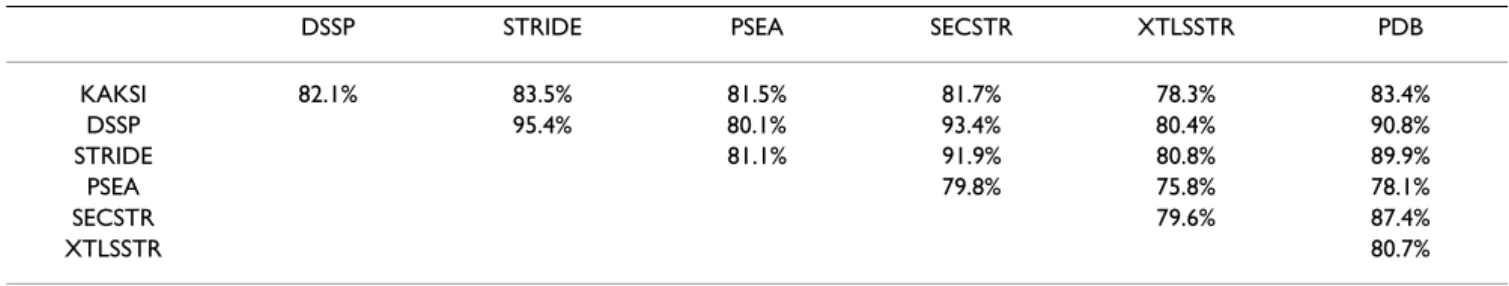
Table 3 shows the C3 scores obtained for the HRes set (the

overall agreement between the different assignment meth-ods show the same tendencies for the different comparison

sets, [see Additional file 1]). A group of methods shows a

strong agreement: C3 scores within the group DSSP,

STRIDE, SECSTR and PDB are all in the range 87.4% (SECSTR versus PDB) to 95.4% (STRIDE versus DSSP).

Table 2: Secondary structure content according to different assignment methods. %H: percentage of residues assigned in α-helix. %b: percentage of residues assigned in β-strand. See the text for β-strand assignment with kaksi using different parameter values on the

LRes and the NMR sets.

Dataset HRes set MRes set LRes set NMR set

Method %H %b %H %b %H %b %H %b KAKSI 36.8 22.0 38.0 22.5 35.1 19.0 33.5 15.2 PDB 40.5 20.3 41.7 20.9 39.3 18.2 35.5 17.3 DSSP 35.9 22.5 37.3 22.9 35.4 20.4 32.2 17.3 STRIDE 36.4 22.6 38.6 23.3 36.3 21.2 33.7 18.8 PSEA 32.1 23.7 34.2 25.0 33.0 24.4 30.6 22.8 SECSTR 37.2 20.1 38.5 20.4 37.0 18.6 33.3 16.3 XTLSSTR 40.4 19.7 40.9 19.6 35.9 14.4 34.3 14.8

The strong similarity between DSSP and STRIDE assign-ments, which both used a hydrogen-bond criterion, has been noted in previous studies [27,29,34]. The SECSTR method is strongly related to the DSSP algorithm and log-ically belongs to this group. As was expected, PDB descrip-tions are very close to DSSP assignments due to the way secondary structure assignments are performed.

Assignments given by XTLSSTR are the most different

from others: C3 scores with DSSP, STRIDE, SECSTR and

PDB are all below 81%. KAKSI and PSEA show an inter-mediate behavior of the other methods [see Additional file 2]. The C3 scores are all in the same range, between

81.5% (KAKSI/PSEA) and 83.5% (KAKSI/STRIDE), excluding XTLSSTR (78.3%).

SOV criterion

The SOV criterion is usually employed for secondary structure prediction evaluation, whereas here, compari-sons are made between alternative structure assignments. SOV values depend on which structure ischosen as refer-ence. To allow comparison, KAKSI is taken as referrefer-ence. Table 4 shows SOV values computed from the HRes set for helices and strands, between KAKSI and other methods. SOV values for other datasets are available, [see Addi-tional file 3].

For helical segments, the highest SOV with KAKSI assign-ment is obtained with DSSP (91.7%). It lies in the same range for STRIDE. It is slightly lower for other methods but remains above 87%. For the strands, a good agree-ment is seen with DSSP, STRIDE and PDB (SOV scores about 90%). Lower SOV (about 83%) are found with PSEA and SECSTRC. Moderate agreement is seen with

XTLSSTR (75.8% only). C3 score between XTLSSTR and

KAKSI is only 78.3%(see table 3). SOV values are high for helices and slightly lower for strands, showing that

differ-ences between both methods mainly concern β-sheets

assignments. Hereafter we will restrict our comparisons to KAKSI, STRIDE, and PSEA assignments on the HRes set. STRIDE is a widely-used method whose results are very

similar to DSSP and PDB, as shown by the C3 scores.

STRIDE is chosen because it exhibits the largest C3 score

with KAKSI. PSEA is chosen because its algorithm fairly differs from other methods, but SOV values remain con-sistent when compared to KAKSI'S.

Segment length distribution

The length distributions of helices and strands assigned by KAKSI, PSEA and STRIDE on the HRes set are shown on Figure 3.

In helix distributions, three zones can be distinguished. (i) For helices shorter than 8 residues, the distributions are very different: STRIDE assigns many 3 residue long

Table 3: C3 scores between different methods on the HRes set

DSSP STRIDE PSEA SECSTR XTLSSTR PDB

KAKSI 82.1% 83.5% 81.5% 81.7% 78.3% 83.4% DSSP 95.4% 80.1% 93.4% 80.4% 90.8% STRIDE 81.1% 91.9% 80.8% 89.9% PSEA 79.8% 75.8% 78.1% SECSTR 79.6% 87.4% XTLSSTR 80.7%

Table 4: SOV measures between kaksi and other methods on the HRes set. SOV_H: SOV for α-helix. SOV_b: SOV for β-strand. KAKSI is taken as reference.

Method SOV_H SOV_b

DSSP 91.7% 92.1% STRIDE 91.2% 91.9 % SECSTR 89.0% 83.9% PSEA 87.5% 82.7% XTLSSTR 89.3% 73.4% PDB 88.4% 89.4%

Length distribution of helices and strands assigned by stride, psea and kaksi

Figure 3

Length distribution of helices and strands assigned by stride, psea and kaksi. Length distribution of helical (top) and

extended (bottom) segments assigned by STRIDE (plain line and crosses), PSEA (dashed line and open circles), and KAKSI (dot-ted line and filled circles), on the HRes set. The STRIDE assignment generates a large number of 3 residue-long helices (1238 segments) and 1 residue-long strands (corresponding to 1800 β-bridges).

Helices

length

frequency

0

4

8

12

16

20

24

28

0

100

300

500

700

Strands

length

frequency

0

4

8

12

16

20

0

200

600

1000

1400

helices, whereas PSEA and KAKSI do not assign helices shorter than 5 residues. PSEA assignments results in slightly larger number of short helices than STRIDE. KAKSI distribution shows a very high peak at 7 residues. (ii) In the range 8 to 15 residues, small differences are observed: KAKSI distribution shows a peak about 12 resi-dues, unlike PSEA and STRIDE distributions. (iii) For hel-ices longer than 15 residues, distributions are similar. Similarly, 3 distinct zones appear in the strand distribu-tions. (i) Up to 6 residues, PSEA and KAKSI curves show larger peaks than STRIDE distribution, at 3 to 5 residues for KAKSI, and 4 and 5 residues for PSEA. PSEA and KAKSI do not assign strands shorter than three residues, whereas STRIDE assignment result in a large number of 1-residue long strands. These segments are isolated β-bridges (state b in stride assignments). (ii) Between 6 and 9 residues, psea and KAKSI segments are more numerous than STRIDE segments. (iii) After 9 residues, the distributions are identical.

Global measures, such as C3 and SOV scores, show that

KAKSI assignments are globally consistent with those given by other existing methods. The length distributions of helices and strands indicates that segment distribution is also roughly similar across methods. This broad consen-sus was expected. In the following sections we now turn toward the study of details of the assignments, in particu-lar, as mentioned in the introduction, we compare the way different methods deal with the edges of secondary structures and cope with local distorsions.

Detailed comparison Pair length

The SOV criterion is a measure of the global overlapping of secondary structure segments. It gives no information about the effect of length of segments or about the respec-tive length of facing segments. Figure 4 shows the plot of lengths for pair of corresponding repetitive structure seg-ments between STRIDE and KAKSI, and PSEA and KAKSI assignments. The pairs are those used for the SOV compu-tation: a pair is considered when there is at least one resi-due in the same state for the two assignments. Unpaired segments are ignored.

Taking KAKSI assignment as our reference, three different cases occur: (i) One segment according to KAKSI corre-sponds to a single segment in another method assign-ment: these are one-to-one events. (ii) One segment assigned by KAKSI corresponds to two or more segments in another method assignment. We call this a fusion event. (iii) The symmetric case, several segments in KAKSI assignment corresponding to a single segments in another method assignment, is called a division event. The three

cases are available plotted on separate graphs [see Addi-tional file 4].

Helix length

The strong accumulation of points along the diagonal, on both plots (KAKSI versus STRIDE and KAKSI versus PSEA) and for every segment lengths shows that KAKSI often agrees with other methods about the length of helices. There are more points below the diagonal than above, indicating that KAKSI tends to assign slightly longer seg-ments than STRIDE and PSEA (one or two residue longer). This occurs for all segment lengths, but it is more striking on the PSEA/KAKSI comparison.

The points appearing far from the diagonal correspond to

division and fusion events, as shown by the squared correla-tion coefficients r2_{. Correlations are calculated on the}

pairs (PSEA or STRIDE length/KAKSI length) and are used as indicators for the dispersion about the diagonal. On the

KAKSI/STRIDE comparison, r2 _{= 0.28 for all the 5146}

pairs, but reaches 0.88 when only the 3755 one-to-one

events are considered. The remaining pairs correspond to 142 cases of fusion and 1249 cases of division events.

Divi-sion events are responsible for the numerous observations of pairs of short helices in KAKSI assignment (5 to 9 resi-dues) with longer helices in PSEA and STRIDE assign-ments (10 to 20 residues).

Similarly, for the KAKSI/PSEA comparison there are 4762 pairs (r2 _{= 0.23), distributed in 3443 one-to-one events (r}2 ₌

0.85), 150 fusion and 1169 division events. Numerous cases of divisions appear on the plot as pairs of 5 to 9 residue helices for KAKSI and 10 to 20 residue helices for PSEA. For both comparisons (KAKSI/STRIDE and PSEA/KAKSI), the number of division events is greater than the number of

fusion events, showing that KAKSI tends to split long segments into shorter ones. This is a direct consequence of the kink detection mechanism used in KAKSI. It also explains why short helices are more abundant in KAKSI assignments than in STRIDE and PSEA. Some examples of this phenomenon are illustrated in Fig 5.

Strand length

The situation is less clear than for helices. The points are more dispersed and there is no clear accumulation of points accounting for division events. In the KAKSI/STRIDE comparison, the 5974 pairs yield a r2 _{equal to 0.35. This}

value increases to 0.69 when only the 5403 one-to-one

events are considered. Amongst the remaining pairs 214 correspond to fusion events, and 357 to division events. The splitting of long segments is thus less systematic than for helices. This makes senses since there is no mechanism similar to the kink detection in helices for β-strands. 52% of the one-to-one events fall above the diagonal (longer

segments in KAKSI assignment) and 22 % fall below the diagonal (shorter segments in KAKSI assignment). The

remaining 26% are on the diagonal. It shows that KAKSI tend to assign longer strands than STRIDE.

Length for pair of segments assigned by stride vs kaksi and psea vs kaksi

Figure 4

Length for pair of segments assigned by stride vs kaksi and psea vs kaksi. Length for pair of helices (upper part) and

strands (lower part) when comparing STRIDE and KAKSI assignments, and PSEA and KAKSI assignments. We report a pair when we found at least one residue in the same state in both assignments. Data are shown as a "sunflower plot": a point stands for a single observation, then the number of "leaves" is proportional to the number of additional observations. The diagonal x = y (same length for two assignments) is shown.

In the KAKSI/PSEA comparison, r2 _{equals 0.23 on the}

5041 pairs and 0.44 on the 4694 one-to-one events. There are 214 fusion events and 133 division events. The numbers of division and fusion events are close, indicating that there only a slight splitting effect. 27% of the one-to-one events are on the diagonal, 50% are above (greater length in PSEA assignment) and 23% are below (greater lenght in

kaksi assignment). In a majority of case, KAKSI assigns shorter strand segments concerning one-to-one events. For both kind of segments and both comparisons, we also checked for the existence of systematic shifts of the seg-ments toward the N-ter or C-ter termini of the secondary

structure elements. No such systematic bias was found (data not shown).

Helix geometry analysis with HELANAL

In KAKSI we pay a special attention to the detection of kinks in α-helices by applying angle and axis criteria. This motivates the study of the geometry of helices with an external tool, according to alternative definitions of helix locations. We check the geometry of helices assigned by the different assignment methods with the HELANAL software. We are interested in the distribution of helices into the three classes: linear (L), curved (C) or kinked (K). Unclassified helices represent less than 1% in our datasets.

Examples of disagreement between kaksi and stride

Figure 5

Examples of disagreement between kaksi and stride. The divergent assignments are drawn in cartoon representation

and highlighted in purple (helix and strand) and cyan (coil assigned by KAKSI). Images are generated with Molscript [46]. Aver-age bending angles (AverBA) between local axes computed by HELANAL in long helices are reported, (a): hemoglobin I from the clam Lucina pectinata, PDB code:1b0b, resolution 1.43 Å. STRIDE assignment: α-helix from residues 4 to 35, AverBA = 15.4°. KAKSI assignment: two helices from 4 to 19, AverBA = 3.84° and 21 to 34, AverBA = 9.0°. (b): chain A of L(+)-mandelate dehydrogenase from Pseudomonas putida, PDB code: 1p4c, resolution 1.35 Å. STRIDE assignment: helix from 308 to 340,

AverBA = 24.7°. KAKSI assignment: two helices from 308 to 315 and 320 to 341, AverBA = 4.3°. (c): chain B of C-phycocyanin

from the thermophylic cyanobacterium Synechococcus elongatus, PDB code: 1jbo, resolution: 1.45 Å. STRIDE assignment: helix from residues 21 to 62, AverBA = 13.1°. KAKSI assignment: 3 helices from 21 to 33, AverBA = 4.5°, 35 to 46, AverBA = 3.0°, and 48 to 61, AverBA = 6.6°. (d): chain A from endo-xylanase from Clostridium stercorarium, PDB code: 1od3, resolution: 1 Å. STRIDE assignment: two β-strands from 61 to 82 and 116 to 135. KAKSI assignment: four β-strands from 61 to 69, 75 to 83, 115 to 122, and 128 to 136. (b) STRIDE (b) KAKSI KAKSI STRIDE (a) (d) STRIDE KAKSI KAKSI STRIDE (c)

When analyzed by HELANAL, helices assigned by all methods show a high proportions of kinks. On the HRes

set, for example, about 20% (DSSP, STRIDE, KAKSI) up to

30% (SECSTR, XTLSSTR) helices appear classified as kinked. This ratio is 16% only for the PDB assignments, and less than 10% for PSEA. When the resolution gets worse, this proportion increases [see Additional file 5]. On the NMR set, we observe as much as 40% kinked heli-ces for PSEA assignment and more 50% kinked heliheli-ces for STRIDE, SECSTR and PDB.

This high ratio of irregular helices (curved or kinked) is in agreement with previously published results [17]. How-ever, the high ratio of kinked helices found here is larger than previously reported by Kumar and Bansal [19]. There is a difference between Kumar and Bansal's work and our study: they modified helix assignment given by DSSP before submission to HELANAL. Using distance and axis

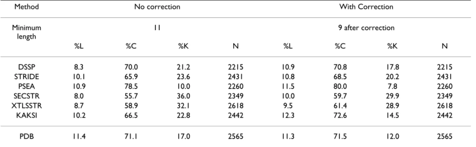
criteria, they corrected helix boundaries to avoid distor-tions at the termini. Consequently, the high ratio of kinked helices is likely due to these terminal residues. Rather than applying the correction used by Kumar and Bansal, we apply a systematic correction before submitting helices to HELANAL, i.e., one residue is removed at each helix terminus. The reason for applying a systematic correction rather than a correction based on geometrical criteria is that we want to make a statistical comparison of helices assigned by various softwares. The goal is not to correct potentially wrong helices bounda-ries. We want to evaluate the assignments as they are pro-duced by the softwares and used in later applications. Table 5 shows the results obtained on the HRes set, before and after correction, for helices defined by the seven methods. Results for other datasets are available [see Additional file 5].

As HELANAL can handle only helices longer than nine residues, we restrict our analysis to helices longer than eleven residues. When removing the first and last residues of helices, the ratio of kinked helices decreases, showing that part of the kinks are due to distortion at the termini. After correction, the geometry of helices assigned by KAKSI (14.5% of kinked helices) is the closest to the geometry of helices described in the PDB (12% kinked helices). The KAKSI method also assigns the highest ratio of linear helices (12.3%). PSEA has only 7.8% kinked hel-ices but it should be noted that the number of helhel-ices sub-mitted to analysis is slightly lower.

It is interesting to investigate the geometry of helices when KAKSI assigns several helices in a region where STRIDE assign a single long helix, i.e., the division events. If we

con-sider the division events involving pair of helices longer than nine residues, we find 128 pairs where a kinked helix assigned by stride corresponds to curved or linear helices assigned by KAKSI. The symmetric case, kinked helices in KAKSI assignment paired with a curved or linear helices in STRIDE assignment concerns only 7 cases. This indicates that splitting long helices into several short ones helps to define helices devoid of kink.

All these observations suggest that the kink detection implemented in KAKSI is efficient and leads to more reli-able helix locations. The major feature of KAKSI assign-ments is then the geometry of α-helices: while assigning slightly longer helices than stride, the global geometry of helices remains satisfactory, with more linear helices than other assignments and a limited ratio of kinked helices,

Table 5: Helix geometry analyzed by HELANAL on the HRes set. Correction: assignments are corrected by shortening each helix by one residue at each terminus. %L: percentage of helices that are linear according to HELANAL. %C: percentage of helices that are curved according to HELANAL. %K: percentage of helices that are kinked according to HELANAL. N: number of helices submitted to HELANAL.

Method No correction With Correction

Minimum length 11 9 after correction %L %C %K N %L %C %K N DSSP 8.3 70.0 21.2 2215 10.9 70.8 17.8 2215 STRIDE 10.1 65.9 23.6 2431 10.8 68.5 20.2 2431 PSEA 10.9 78.5 10.0 2260 11.5 80.0 7.8 2260 SECSTR 8.0 55.7 36.0 2349 10.0 59.7 29.9 2349 XTLSSTR 8.7 58.9 32.1 2618 9.5 61.4 28.9 2618 KAKSI 10.2 66.5 22.8 2442 12.3 72.6 14.5 2442 PDB 11.4 71.1 17.0 2565 11.3 71.5 12.0 2565

very close to PDB assignments. This is accomplished by dividing long distorted helices when appropriate. Some examples are shown in the following section.

Some examples of assignment disagreements

Figure 5 shows some interesting examples of disagree-ment between STRIDE and KAKSI assigndisagree-ments. The first three examples in Figure 5 concern disagreement about helix assignments. In example (a), the long helix assigned by STRIDE shows a sharp kink. In KAKSI assignment it is replaced by two helices from residues 4 to 19 and 21 to 34. The first helix is classified as curved by HELANAL. The second one is classified as kinked, but it becomes linear after removal of terminal residues. The angle between two global axes fitted in these two helices is 83°. The second example (b), is even more striking: a 33-residue long helix defined by STRIDE from residues 308 to 340 exhibits a reverse turn near its N-terminal edge. The definition given by KAKSI is two helices from 308 to 315 and 320 to 341. The first helix is too short to be analyzed by HELANAL and the second one is classified as linear. The third exam-ple is the case of a division of a long helix assigned by STRIDE into three segments in KAKSI assignment. Although less marked than for the first two examples, the kinks are well apparent. The three helices defined by KAKSI are all classified as curved by HELANAL, with their global axes making angles equal to 135 and 120° between the first and the second, and the second and the third helix respectively.

The last example 5(d) is an example of disagreement on a

β-strands assignment. β-strands assigned by STRIDE are

fairly curved, allowing a change of direction of the back-bone. No specific routine is implemented in KAKSI to split distorted strands, as it is done for helices. Nonethe-less, the criteria of β-sheet assignment being fairly strict, some cases of division in long β-strands can also occur. These examples illustrate the fact that a small disagree-ment on a per-residue basis can result in a radical change in the structure description. In the examples shown on Fig. 5 we believe that KAKSI assignments provide a more pertinent description of the protein structure.

Conclusion

We have developed a new automatic procedure to assign secondary structures from 3D coordinates. Our method,

KAKSI, uses Cαdistances and (Φ/Ψ) angles and pay a

spe-cial attention to kink detection in helices. Like other methods (except PSEA), it is sensitive to the resolution, and the type of experimental technique used to solve the structure. Consequently, we propose to choose detection parameters according to the structure resolution or tech-nique and the nature of the secondary structure, since β -sheets are more difficult to detect. The careful comparison of KAKSI assignments with assignments produced by five

available methods and the description provided by the PDB highlights the similarities and differences between the different methods. Good general agreement are

observed between methods, especially on α-helices. The

length of α-helices and β-strands, in case of agreement on the number of segments, are very similar when compared to STRIDE and PSEA. When different lengths are assigned, we observe slightly longer α-helices and β-strands than the STRIDE definition. When two methods disagree on the number of segments, we observe more division events than fusions, i.e., several short helices assigned by KAKSI in front of a unique long helix assigned by STRIDE or PSEA.

Division events are also slightly predominant in the

com-parison of β-strand length with STRIDE and PSEA. The

study of α-helix geometry with an external tool reveals

that KAKSI helices are less kinked that helices assigned by other methods, except PSEA. KAKSI is also the method that assigns helices with geometrical characteristics in best agreement with helices described in the PDB, and, maybe more important, the highest proportion of linear helices. As stated by Andersen and co-workers [35], each method reflects its own definition of secondary structures. Our definition favors a certain regularity of secondary structure elements, as illustrated by the examples on Fig. 5.

Methods

Datasets

The KAKSI method uses geometrical characteristics of α

-helices and β-sheets extracted from available protein

structures. A reference set (Ref set), consisting of 2880 structural domains taken from ASTRAL 1.63 [36] is used to estimate these geometrical characteristics. The list of domains with less than 40% identity provided by the ASTRAL server [37] is filtered to keep only X-ray structures with a resolution better than 2.25 Å and longer than 50 residues.

KAKSI assignments are compared with secondary struc-ture assignments done by other methods. For the reasons mentioned above four different sets of structures are used. Hereafter we refer to these datasets as the Comparison sets. The number of structures reported below refer to the files that are successfully processed by all assignment programs and contain a secondary structure description provided by the PDB.

• A High Resolution set (HRes set): X-ray structures with resolution better than 1.7 Å, R-factor < 0.19, identity per-centage between sequences less than 30%, obtained from the WHATHIF website [38,39]. There are 689 structures in this set, corresponding to 151922 residues with a defined secondary structure, i.e., excluding missing coordinates.

• A Medium Resolution set (MRes set): X-ray structures with resolution between 1.7 Å and 3 Å, R-factor < 0.3, identity percentage between sequences less than 30%, minimum length of 40 residues, provided by the PISCES website [40,41]. There are 624 structures in this set, corre-sponding to 160 276 residues with a defined secondary structure.

• A Low Resolution set (LRes set): X-ray structures with res-olution worse than 3 Å, R-factor > 0.3, identity percentage between sequences less than 30%, minimum length of 40 residues, provided by the PAPIA website [42]. There are 332 structures in this set, corresponding to 97852 residues with a defined secondary structure.

• A NMR set: structures with less than 30% sequence iden-tity, extracted from all NMR entries obtained on the PDB website [43]. The redundancy of the set is reduced to 30% sequence identity with PISCES. There are 296 structures in this set, corresponding to 27533 residues with a defined secondary structure.

These lists are available on the web [see Additional file 6].

KAKSI method

The assignment of repetitive secondary structures by KAKSI is based on a set of characteristic values of Cα dis-tances and (Φ/Ψ) dihedral angles. The parameters of KAKSI have been chosen to best fit the secondary structure assignments obtained from the PDB files (HELIX and SHEET fields). These fields, when present, are automati-cally generated with the DSSP method or are provided by the depositor who might have used some secondary struc-ture assignment program and/or might have inspected visually the 3D structure and assigned himself the second-ary structures. We use these PDB assignments as our gold-standard for the sake of parameter calculations, keeping in mind that the data are partly similar to DSSP assignments. Assignment is done by sliding windows along the

sequence. α-helices are assigned first, followed by β

-sheets. Two windows are slid for the β-sheet detection

because we only want to assign β-strands involved in β

-sheets. Residues once assigned in α-helix cannot be

re-assigned in β-sheets.

Secondary structure characteristics used by the KAKSI heuristic

As mentioned earlier, α-helices and β-strands being peri-odic structures, their backbone geometry exhibits a number of regularities. This periodicity leads to character-istic distances between Cαatoms as well as characteristic values of (Φ/Ψ) dihedral angles.

More precisely, we have estimated from the Ref set:

• distances between Cα in α-helices and β-sheets. Different statistical distributions are computed for terminal resi-dues and cores of secondary structure segments because greater variations are observed at segment termini. For α -helices, 4 distances are considered between residues i and

j along the sequence, with j 苸 [i + 2, i + 5]. Table 1 shows the means and standard deviations obtained on the Ref

set. For β-sheets, three different types of distances are considered. Figure 1 illustrates these distances and reports the values obtained on the Ref set.

• (Φ/Ψ) values for residues involved in α-helices and β -strands. Densities of (Φ/Ψ) angles are computed using Ramachandran maps. These maps are divided into 10 by 10 degree squares. This yields two population maps: one specific of α-helices and the other specific of β-strands [see Additional file 7]. For the α-helix map, we only consider angles lying in the area (Φ < 0° and -90° < Ψ < 60°) and we set to zero square frequencies that are too low (fre-quency <δH). In this study, the threshold δH is fixed,

empirically, to 20 × nmean, nmean being the mean frequency

for a square in the Ramachandran map.

As mentioned above we are particularly interested in the detection of kinks in α-helices. Kinks are frequent and not easy to detect with usual distance and angle criteria. In a regular helix, (Φ/Ψ) angles should remain located in a narrow region of the Ramachandran map. One way to detect kinks (criterion K1 below), is to compute distances between (Φ/Ψ) pairs of successive residues j and j + 1 in the Ramachandran map. We use the 95-percentile of the distance distribution in α-helices. The kink detection is only performed in helix cores, terminal residues of seg-ments being disregarded in the computation.

KAKSI heuristic for helix and strand assignment

Figure 2 illustrates the heuristic implemented in KAKSI. We have tested several criteria and combinations of crite-ria. The final heuristic presented here shows a good agree-ment with PDB assignagree-ments. The principle of the assignment is to test the Cαdistances along the protein to check if they are close to the typical distances in regular secondary structure. The (Φ/Ψ) angles are tested in the same manner. α-helix assignment is achieved according to

a distance or an angle criterion. The β-sheet detection

requires the satisfaction of both angle and distance crite-ria. α-helix assignments are corrected whenever kinks are detected. Criteria applied at each step shown on Figure 2 are explained below, in the order they appear in the assignment process. Characteristic values extracted from the Ref set are shown in capital. The parameters of the method are : ε_H and ε_b are used to define thresholds for Cα

distances and η_H and σ_b are used to define thresholds for the constraints on (Φ/Ψ) angles.

• Distance criterion for α-helices (C1). All Cαdistances in a sliding window of length w1 (fixed to 6 in this study) must

lie within the interval [Mα - εH × SDα; Mα+ εH × SDα]. Mα

and SD_α represent the mean and standard deviation of Cα

distance distributions in α-helices.

• Angle criterion for α-helices (C2). All (Φ/Ψ) pairs in a

slid-ing window of length w2 (fixed to 4 in this study) must

satisfy the condition (Φ < 0° and -90° < Ψ < 60°) and one pair at least must fall in the highly populated zone of the population matrix, i.e with density> δ_H.

• Kinks in α-helices are detected using two criteria.

- Kink criterion K1 is based on the values of (Φ/Ψ) dihe-dral angles. A helix is interrupted at residue j + 1 if the sum

dΦ/Ψ (j, j + 1) + dΦ/Ψ (j + 1, j + 2) is greater than

. dΦ/Ψ (j, j + 1) is analogous to the root mean

square deviation on angular value described by Shuch-hardt and coll [44]. It measures the distance between dihedral angle pairs of residues j and j + 1 in the

Ramach-andran map. is the 95-percentile of the

distribu-tion of such distances.

- Kink criterion K2 relies on axes. An axis is fitted along the helix, by minimizing the function with n the number of residues in the helix, di the distance from the ith Cαto the axis, and d_m the mean of the dis. For a perfect (linear) helix the value

of Daxis is zero and the corresponding vector is the axis of

the cylinder circumscribed by backbone atoms. A helix is interrupted if it appears better to fit it with two axes. These

Typical Cα distance in β-sheets

Figure 1

Typical Cα distance in β-sheets. Typical Cα distances computed from the Ref set in parallel (left part) and anti-parallel β -sheets. Mean distances are indicated in Å with their standard deviations within parentheses. Separate statistics were computed for distances involving only residues in strand cores (italic) and distances involving residues at strand edges (bold). For the intra-strand distance (type i to i + 2), no distinction is made on the sheet orientation.

Table 1: Distances in α-helices. Core: distances not involving residues at helix edge. Termini: distances involving at least one residue at helix edge. Mean distances, computed on the HRes set, are indicated in Å with their standard deviations within parentheses.

Type Core Termini

i to i + 2 5.49(0.20) 5.54(0.25) i to i + 3 5.30(0.64) 5.36(0.39) i to i + 4 6.33(0.71) i to i + 5 8.72(0.63)

i+2

i+1

i

j+1

4.88(0.43)

4.77(0.42)

j

j+2

i+2

i+1

j

i

j+1

j+2

4.83(0.29) 4.84(0.24)

6.70(0.32)

6.07(0.35)

6.70(0.32)

6.00(0.47)

∑

two axes must make an angle greater than θ_k (θ_k fixed to 25° in this study).

• Distance criterion for β-sheets (C3). All the Cαdistances in two sliding windows of length w3 (here w3 = 3) must be in

the interval [Mβ - εb × SDβ; Mβ + εb × SDβ]. Mβ and SDβ

rep-resent the mean and standard deviation of Cα distance

distributions in β-sheets.

• Angle criterion for β-sheets (C4). For each (Φ/Ψ) angle pair falling in the populated zone of the Ramachandran map (density > 0), we increment a counter score(sheet) by 1. If a (Φ/Ψ) angle pair of the central residue of a sliding window verifies -120° < Ψ < 50°, then score(sheet) is reset to zero. The final score(sheet) must be greater or equal to σ b.

• Contiguous segments correction, criterion (C5). If a helix and a strand are adjacent, a coil is introduced in between, shortening the helix by one residue.

Empirically, the optimal parameter values are: ε_H = 1.96,

ηH = 2.25, εb = 2.58 and σb = 5.

Comparative methods for secondary structure assignment and reduction to three states

KAKSI assignments are compared to the assignments given by five available methods on the Comparison sets: DSSP [21], STRIDE [23], PSEA [27], XTLSSTR [28] and SECSTR [24]. HELIX and SHEET records in PDB files are also considered as an independent assignment method. When needed, secondary structure assignments are reduced to three classes (H for α-helix, b for β-strand, c for

Flow-chart of the kaksi heuristic for secondary structure assignment

Figure 2

Flow-chart of the kaksi heuristic for secondary structure assignment. Minimum length for helices is set to LH = 5. The

criteria C1, C2, C3, C4, C5, K1 and K2 are detailed in the text.

Secondary structure assignment

Secondary structure

satisfied ? C3 with a sliding window

with a sliding window

yes

yes

Scan the helices for kink detection

yes

for all residues in

Assign a coil state

yes

for all residues yes INPUT

and discard helix OUTPUT

Scan the sequence

of length w Scan the sequence

Scan the sequence in non−helical state

with two sliding windows

Correct contiguous

distance criterion angle criterion distance criterion

Assign helical state for all residues in

the window

Assign helical state

the window

and discard helix at the distorded residue

Is the

angle criterion satisfied ?

Assign extended state

in both windows Is the Is the or ? a distorsion detected Is there C coordinates Is the α angles Φ/Ψ of length w 1 2 of length w₃ Helix assignment Helix correction Sheet assignment no no no no no by criteria K1 C4 C5 of lenth of lenth K2 l<L H l<L_H

segments with criterion

satisfied ? C1

satisfied ? C2

coil) as follows: DSSP, STRIDE and SECSTR: (H,G,I) = H, (E,b) = b, others (S,T,blank) = c; XTLSSTR: (G,g,H,h) = H, (E,e) = b, others (T,N,P,p,-) = c. PSEA assigns only three states. XTLSSTR possibly provides several alternative assignments for one residue. In that case, only the first assignment is considered. When dealing with NMR struc-tures, only the first model is analyzed.

Comparison measures Secondary structure content

The secondary structure content of a dataset is measured by the percentage of residues involved in the three struc-tural classes: α-helix, β-strand and coil.

Overall agreement

The C3 score is the percentage of residues assigned in the

same state when comparing two different assignments: C3

= Nid/Ntot with Nid the number of residues for which both

assignments are identical, and Ntot the total number of

res-idues with defined secondary structure. It is analogous to

the Q3 score used to evaluate secondary structure

prediction.

Segment based-agreement

• The mean agreement based on secondary structure seg-ments is measured by the percentage of Segment OVerlap (SOV). We use the SOV definition described by Zemla and coworkers [45]. For state i (α-helix, β-strand or coil) the segment overlap measure is defined as:

with the normalization value N(i) defined as:

The sums on S(i) are taken over all the segment pairs in state i which overlap by at least one residue. The sum on

S'(i) is taken over the remaining segments in state i found in the reference assignment 1, len(s1) is the number of

res-idues in segment s1, minov(s1, s2) is the length of overlap

of s1 and s2, maxov(s1, s2) is the total extend for which

either of the segments S1 and s2 has a residue in state i, and delta(s1, s2) is defined as:

min {maxov(s1, s2) - minov(s1, s2); minov(s1, s2); int(len(s1)/

2); int(len(s2)/2)},

where min {x1; x2; x3;...; xn} is the minimum of n inte-gers. This formula is usually employed to compare a

sec-ondary structure prediction (S2) with a secondary

structure description (S1) taken as reference. The roles of S₁ and S2 are thus not symmetrical.

• Length of pair of segments used for the SOV computa-tion are collected. A pair is defined each time there is at least one residue in common between assignment X and Y. Unpaired secondary structure elements are ignored in this analysis. These length pairs can be viewed on a bi-plot (length(X) versus length(Y)).

Helix geometry analysis with an external software

The HELANAL software developed by Kumar and Bansal [33] is dedicated to helix geometry analysis. HELANAL takes as input a PDB file and a description of helix bound-aries. It calculates local axes every four residues. The geometry of a helix is determined by the angles between axes and the goodness of fit of the helix trace with a circle or a line. Helices are then classified as kinked (K), linear (L) or curved (C). HELANAL can leave a helix unclassified if its geometry is ambivalent. The minimum length for a helix to be analyzed is nine residues.

In this study, HELANAL is used as an external control of helix geometry. All α-helices in the comparison sets are sub-mitted to HELANAL analysis. Different assignment meth-ods are used to provide alternate definition of helices boundaries.

Availability and requirements

• Project home page: http://migale.jouy.inra.fr/mig/ mig_fr/servlog/kaksi/

• Operating system: Linux • Programming langage: C

• Other requirements: libxml2 >= 2.6, see ftp://xml-soft.org/

• License: GNU GPL

• Any restrictions to use by non-academics: no

• Implementation: the software is composed of 2 pro-grams: KAKSI takes a PDB file as input and prints the assigned secondary structure (and other data of intereset) in an XML output K2R reads a KAKSI XML output file and outputs the data in various FASTA format files by default. K2R allows users to easily implement any new output mat they whish. a lot of different informations in raw for-mats (mainly FASTA format).

The source code is available on the project home page.

SOV i N i s s delta s s s s len s i ( ) ( ) ( , ) ( , ) ( , ) ( ) = 1

_∑

∑

∑

List of abbreviations used

3D: three-dimensional, Cα: backbone α-carbon, NMR:

Nuclear Magnetic Resonance, PDB: Protein Data Bank.

Authors' contributions

JM and AM developped the program. GL carried out the comparison between different assignments. JM GL and JFT carried out the analysis. JM, AdB and JFG conceived the study and participated in its design and coordination

Additional material

Acknowledgements

This research was funded in part by the 'ACI Masse de données'. We are grateful to INRA for awarding a doctoral Fellowship to JM and to the

Min-istère de l'Education Nationale, de l'Enseignement supérieur et de la Recherche for awarding a doctoral Fellowship to JFT.

References

1. Pauling L, Corey RB, Branson HR: The structure of proteins; two

hydrogen-bonded helical configurations of the polypeptide chain. Proc Natl Acad Sci USA 1951, 37(4):205-211.

2. Pauling L, Corey RB: The pleated sheet, a new layer

configura-tion of polypeptide chains. Proc Natl Acad SciU S A 1951, 37(5):251-256.

3. Gibrat JF, Madej T, Bryant SH: Surprising similarities in structure

comparison. Curr Opin Struct Biol 1996, 6(3):377-385.

4. Murzin AG, Brenner SE, Hubbard T, Chothia C: SCOP: a structural

classification of proteins database for the investigation of sequences and structures. J Mol Biol 1995, 247(4):536-40.

5. Orengo CA, Michie AD, Jones S, Jones DT, Swindells MB, Thornton JM: CATH-a hierarchic classification of protein domain

structures. Structure 1997, 5(8):1093-1108.

6. Sayle RA, Milner-White EJ: RASMOL: biomolecular graphics for

all. Trends Biochem Sci 1995, 20(9):374.

7. Humphrey W, Dalke A, Schulten K: VMD: visual molecular

dynamics. J Mol Graph 1996, 14:33-38. 27-28.

8. Sali A, Blundell TL: Comparative protein modelling by

satisfac-tion of spatial restraints. J Mol Biol 1993, 234(3):779-815.

9. Bradley P, Chivian D, Meiler J, Misura KM, Rohl CA, Schief W, R Wedemeyer W, Schueler-Furman O, Murphy P, Schonbrun J, Strauss C, Baker D: Rosetta predictions in CASP5: successes, failures,

and prospects for complete automation. Proteins 2003, 53(Suppl 6):457-468.

10. Pollastri G, Przybylski D, Rost B, Baldi P: Improving the prediction

of protein secondary structure in three and eight classes using recurrent neural networks and profiles. Proteins 2002, 47(2):228-235.

11. Petersen TN, Lundegaard C, Nielsen M, Bohr H, Bohr J, Brunak S, Gippert GP, Lund O: Prediction of protein secondary structure

at 80% accuracy. Proteins 2000, 41:17-20.

12. Jones DT: Protein secondary structure prediction based on

position-specific scoring matrices. J Mol Biol 1999, 292(2):195-202.

13. Frishman D, Argos P: The future of protein secondary structure

prediction accuracy. Fold Des 1997, 2(3):159-62.

14. Rost B: Review: protein secondary structure prediction

con-tinues to rise. J Struct Biol 2001, 134(2–3):204-218.

15. Schulz GE, Barry CD, Friedman J, Chou PY, Fasman GD, Finkelstein AV, Lim VI, Pititsyn OB, Kabat EA, Wu TT, Levitt M, Robson B, Nagano K: Comparison of predicted and experimentally

determined secondary structure of adenyl kinase. Nature

1974, 250(462):140-2.

16. Robson B, Garnier J: Introduction to Proteins and Protein Engineering Amsterdam: Elsevier Press; 1986.

17. Barlow DJ, Thornton JM: Helix geometry in proteins. J Mol Biol 1988, 201(3):601-619.

18. Kumar S, Bansal M: Structural and sequence characteristics of

long alpha helices in globular proteins. Biophys J 1996, 71(3):1574-1586.

19. Kumar S, Bansal M: Geometrical and sequence characteristics

of alpha-helices in globular proteins. Biophys J 1998, 75(4):1935-1944.

20. Levitt M, Greer J: Automatic identification of secondary

struc-ture in globular proteins. J Mol Biol 1977, 114(2):181-239.

21. Kabsch W, Sander C: Dictionary of protein secondary

struc-ture: pattern recognition of hydrogen-bonded and geometri-cal features. Biopolymers 1983, 22(12):2577-637.

22. Berendsen HJC, van der Spoel D, van Drunen R: GROMACS: A

message-passing parallel molecular dynamics implementation. Comp Phys Comm 1995, 91:43-56.

23. Frishman D, Argos P: Knowledge-based protein secondary

structure assignment. Proteins 1995, 23(4):566-579.

24. Fodje MN, Al-Karadaghi S: Occurrence, conformational

fea-tures and amino acid propensities for the pi-helix. Protein Eng

2002, 15(5):353-358.

25. Richards FM, Kundrot CE: Identification of structural motifs

from protein coordinate data: secondary structure and first-level supersecondary structure. Proteins 1988, 3(2):71-84.

Additional File 1

C3 scores for all datasets.

Click here for file

[http://www.biomedcentral.com/content/supplementary/1472-6807-5-17-S1.pdf]

Additional File 2

Graphical views of C3 scores for the HRes set.

Click here for file

[http://www.biomedcentral.com/content/supplementary/1472-6807-5-17-S2.pdf]

Additional File 3

SOV scores for all datasets.

Click here for file

[http://www.biomedcentral.com/content/supplementary/1472-6807-5-17-S3.pdf]

Additional File 4

Length of pairs of helices and strands on separate plots.

Click here for file

[http://www.biomedcentral.com/content/supplementary/1472-6807-5-17-S4.pdf]

Additional File 5

Helix geometry analysis on all datasets.

Click here for file

[http://www.biomedcentral.com/content/supplementary/1472-6807-5-17-S5.pdf]

Additional File 6

Urls to retrieve the list of structures used in this study.

Click here for file

[http://www.biomedcentral.com/content/supplementary/1472-6807-5-17-S6.pdf]

Additional File 7

Φ/Ψ repartition in helices and strands defined by the PDB.

Click here for file

[http://www.biomedcentral.com/content/supplementary/1472-6807-5-17-S7.pdf]

Publish with BioMed Central and every scientist can read your work free of charge

"BioMed Central will be the most significant development for disseminating the results of biomedical researc h in our lifetime."

Sir Paul Nurse, Cancer Research UK

Your research papers will be:

available free of charge to the entire biomedical community peer reviewed and published immediately upon acceptance cited in PubMed and archived on PubMed Central yours — you keep the copyright

Submit your manuscript here:

http://www.biomedcentral.com/info/publishing_adv.asp

BioMed_central

26. Sklenar H, Etchebest C, Lavery R: Describing protein structure:

a general algorithm yielding complete helicoidal parameters and a unique overall axis. Proteins 1989, 6:46-60.

27. Labesse G, Colloc'h N, Pothier J, Mornon JP: P-SEA: a new

effi-cient assignment of secondary structure from C alpha trace of proteins. Comput Appl Biosci 1997, 13(3):291-5.

28. King SM, Johnson WC: Assigning secondary structure from

protein coordinate data. Proteins 1999, 3(35):313-320.

29. Dupuis F, Sadoc JF, Mornon JP: Protein secondary structure

assignment through Voronoi tessellation. Proteins 2004, 55(3):519-528.

30. Berman HM, Westbrook J, Feng Z, Gilliland G, Bhat TN, Weissig H, Shindyalov IN, Bourne PE: The Protein Data Bank. Nucleic Acids

Res 2000, 28:235-242.

31. PDB Format Description Version 2.2 [http://www.rcsb.org/

pdb/docs/format/pdbguide2.2/guide2.2_frame.html]

32. Colloc'h N, Etchebest C, Thoreau E, Henrissat B, Mornon JP:

Com-parison of three algorithms for the assignment of secondary structure in proteins: the advantages of a consensus assignment. Protein Eng 1993, 6(4):377-382.

33. Bansal M, Kumar S, Velavan R: HELANAL: a program to

charac-terize helix geometry in proteins. J Biomol Struct Dyn 2000, 17(5):811-819.

34. Fourrier L, Benros C, de Brevern AG: Use of a structural

alpha-bet for analysis of short loops connecting repetitive structures. BMC Bioinformatics 2004, 5:58.

35. Andersen C, Rost B: Automated Secondary Structure

Assign-ment. In Structural Bioinformatics Edited by: Bourne PE, Weissig H.

Hoboken: Wiley-Liss; 2003:341-363.

36. Brenner SE, Koehl P, Levitt M: The ASTRAL compendium for

protein structure and sequence analysis. Nucleic Acids Res 2000, 28:254-256.

37. ASTRAL website [http://astral.berkeley.edu/]

38. Hobohm U, Scharf M, Schneider R, Sander C: Selection of a

repre-sentative set of structures from the Brookhaven Protein Data Bank. Protein Science 1992, 1:409-417.

39. WHATHIF website [http://swift.cmbi.kun.nl/whatif/select/]

40. PISCES website [http://dunbrack.fccc.edu/PISCES.php]

41. Wang G, Dunbrack RLJ: PISCES: a protein sequence culling

server. Bioinformatics 2003, 19(12):1589-1591.

42. PAPIA website [http://mbs.cbrc.jp/papia/papia.html]

43. PDB website [http://www.rcsb.org/pdb/]

44. Schuchhardt J, Schneider G, Reichelt J, Schomburg D, Wrede P:

Local structural motifs of protein backbones are classified by self-organizing neural networks. Protein Eng 1996,

9(10):833-842.

45. Zemla A, Venclovas C, Fidelis K, Rost B: A modified definition of

Sov, a segment-based measure for protein secondary struc-ture prediction assessment. Proteins 1999, 34(2):220-223.

46. Kraulis PJ: MOLSCRIPT: A Program to Produce Both

Detailed and Schematic Plots of Protein Structures. J Applied