Positive periodic solutions of an epidemic model with seasonality

(1)

Volume 2013, Article ID 470646,10pages http://dx.doi.org/10.1155/2013/470646

Research Article

Positive Periodic Solutions of an Epidemic

Model with Seasonality

Gui-Quan Sun,

1,2,3

Zhenguo Bai,

4

Zi-Ke Zhang,

5,6,7

Tao Zhou,

6

and Zhen Jin

1,2

1_{Complex Sciences Center, Shanxi University, Taiyuan 030006, China}

2_{School of Mathematical Sciences, Shanxi University, Taiyuan, Shanxi 030006, China} 3_{Department of Mathematics, North University of China, Taiyuan, Shanxi 030051, China} 4_{Department of Applied Mathematics, Xidian University, Xi’an, Shaanxi 710071, China} 5_{Institute of Information Economy, Hangzhou Normal University, Hangzhou 310036, China}

6_{Web Sciences Center, University of Electronic Science and Technology of China, Chengdu, Sichuan 610054, China} 7_{Department of Physics, University of Fribourg, Chemin du Mus´ee 3, 1700 Fribourg, Switzerland}

Correspondence should be addressed to Gui-Quan Sun; gquansun@126.com Received 17 August 2013; Accepted 12 September 2013

Academic Editors: P. Leach, O. D. Makinde, and Y. Xia

Copyright © 2013 Gui-Quan Sun et al. This is an open access article distributed under the Creative Commons Attribution License, which permits unrestricted use, distribution, and reproduction in any medium, provided the original work is properly cited. An SEI autonomous model with logistic growth rate and its corresponding nonautonomous model are investigated. For the autonomous case, we give the attractive regions of equilibria and perform some numerical simulations. Basic demographic

reproduction number𝑅_𝑑is obtained. Moreover, only the basic reproduction number𝑅₀cannot ensure the existence of the positive

equilibrium, which needs additional condition𝑅_𝑑 > 𝑅₁. For the nonautonomous case, by introducing the basic reproduction

number defined by the spectral radius, we study the uniform persistence and extinction of the disease. The results show that for the periodic system the basic reproduction number is more accurate than the average reproduction number.

1. Introduction

Bernoulli was the first person to use mathematical method to evaluate the effectiveness of inoculation for smallpox [1–

6]. Then in 1906, Hawer studied the regular occurrence of measles by a discrete-time model. Moreover, Ross [3,

4] adopted the continuous model to study the dynamics of malaria between mosquitoes and humans in 1916 and 1917. In 1927, Kermack and McKendrick [5, 6] extended the above works and established the threshold theory. So far, mathematical models have gotten great development and have been used to study population dynamics, ecology, and epidemic, which can be classified in terms of different aspects. From the aspect of the incidence of infectious diseases, there are bilinear incidence, standard incidence, saturating incidence, and so on. According to the type of demographic import, the constant import, the exponential import, and the logistic growth import are the most common forms. The simple exponential growth models can provide

an adequate approximation to population growth for the initial period. If no predation or intraspecific competition for populations is included, the population can continue to increase. However, it is impossible to grow immoderately due to the intraspecific competition for environmental resources such as food and habitat. So, for this case, logistic model is more reasonable and realistic which has been adopted and studied [7–18]. Moreover, due to its rich dynamics, the logistic models have been applied to many fields. Fujikawa et al. [9] applied the logistic model to show Escherichia coli growth. Invernizzi and Terpin [14] used a generalized logistic model to describe photosynthetic growth and predict biomass pro-duction. Min et al. [15] used logistic dynamics model to describe coalmining cities’ economic growth mechanism and sustainable development. There is a good fit in simulating the coalmining cities’ growth and development track based on resource development cycle. Banaszak et al. [17] investigated logistic models in flexible manufacturing, and Brianzoni et al. [18] studied a business-cycle model with logistic population

(2)

growth. Muroya [13] investigated discrete models of non-autonomous logistic equations. As a result, this paper builds an SEI ordinary differential model with the logistic growth rate and the standard incidence.

For general epidemic models, we mainly study their threshold dynamics, that is, the basic reproduction number which determines whether the disease can invade the suscep-tible population successfully. However, for the system with logistic growth rate, besides the basic reproduction number, the qualitative dynamics are controlled by a demographic threshold𝑅_𝑑 which has a similar meaning and is called as the basic demographic reproduction number. If 𝑅_𝑑 > 1, the population grows; that is, a critical mass of individuals for the disease to spread may be supported. If 𝑅_𝑑 < 1, the population will not survive; that is, not enough mass of individuals may be supported for the disease to spread. For this case, the dynamical behavior of disease will be decided by two thresholds𝑅₀and𝑅_𝑑.

It is well known that many diseases exhibit seasonal fluctuations, such as whooping cough, measles, influenza, polio, chickenpox, mumps, and rabies [19–22]. Seasonally effective contact rate [22–26], periodic changing in the birth rate [27], and vaccination program [28] are often regarded as sources of periodicity. Seasonally effective contact rate is related to the behavior of people and animals, the temper-ature, and the economy. Due to the existence of different seasons, people have different activities which may lead to a different contact rate. Because of various factors, the economy in a different season has a very big difference. Therefore, this paper studies the corresponding non-autonomous system which is obtained by changing the constant transmission rate into the periodic transmission rate. Seasonal transmission is often assumed to be sinusoidal (cosine function has the same meaning), such that𝜆(𝑡) = 𝜆(1 + 𝜂 sin(𝜋𝑡/𝑏)) where 𝜂 is the amplitude of seasonal variation in transmission (typically referred to as the “strength of seasonal forcing”) and2𝑏 is the period, which is a crude assumption for many infectious diseases [29–31]. When 𝜂 = 0, there is no nonseasonal infections. Motivated by biological realism, some recent papers take the contact rate as𝜆(𝑡) = 𝜆(1 + 𝜂 term(𝑡)), where term is a periodic function which is +1 during a period of time and −1 during other time. More natural term can be written as𝜆(𝑡) = 𝜆(1 + 𝜂)term(𝑡)[29]. Here, we take the form 𝛽(𝑡) = 𝑎[1 + 𝑏 sin(𝜋𝑡/10)].

The paper is organized as follows. In Section 2, we introduce an autonomous model and analyze the equilibria and their respective attractive region. InSection 3, we study the non-autonomous system in terms of global asymptotic stability of the disease-free equilibrium and the existence of positive periodic solutions. Moreover, numerical simulations are also performed. InSection 4, we give a brief discussion.

2. Autonomous Model and Analysis

2.1. Model Formulation. The model is a system of SEI

ordi-nary differential equations, where𝑆 is the susceptible, 𝐸 is the exposed, 𝐼 is the infected, and 𝑁 = 𝑆 + 𝐸 + 𝐼. This system considers the logistic growth rate and the standard

Table 1: Descriptions and values of parameters in model (1).

Parameter Interpretation Value

𝑟 The intrinsic growth rate

𝑘 The carrying capacity 100000

𝛽 The transmission rate

𝑚 The natural mortality rate 0.1

𝜎 Clinical outcome rate 0.2

𝜇 The disease-induced mortality rate 0.1

𝑎 The baseline contact rate

𝑏 The magnitude of forcing

incidence which is fit for the long-term growth of many large populations. The incubation period is considered for many diseases which do not develop symptoms immediately and need a period of time to accumulate a pathogen quantity for clinical outbreak, such as rabies, hand-foot-mouth disease, tuberculosis, and AIDS [22,32]. The model we employ is as follows: 𝑑𝑆 𝑑𝑡 = 𝑟𝑁 (1 − 𝑁 𝑘) − 𝛽𝑆𝐼 𝑁 − 𝑚𝑆, 𝑑𝐸 𝑑𝑡 = 𝛽𝑆𝐼 𝑁 − 𝜎𝐸 − 𝑚𝐸, 𝑑𝐼 𝑑𝑡 = 𝜎𝐸 − 𝑚𝐼 − 𝜇𝐼, (1)

where all parameters are positive whose interpretations can be seen inTable 1.

Noticing the equations in model (1), we have 𝑑𝑁

𝑑𝑡 = 𝑟𝑁 (1 − 𝑁

𝑘) − 𝑚𝑁 − 𝜇𝐼. (2) When there exists no disease, we have

𝑑𝑁 𝑑𝑡 = 𝑟𝑁 (1 − 𝑁 𝑘) − 𝑚𝑁 = [𝑟 (1 − 𝑁 𝑘) − 𝑚] 𝑁. (3) Let𝑅_𝑑 = 𝑟/𝑚, if 𝑅_𝑑 > 1, 𝑁 → 𝑁0 = (1 − 𝑚/𝑟)𝑘 for 𝑁(0) > 0, as 𝑡 → +∞; that is, the population will grow and tend to a steady state𝑁0. If 𝑅_𝑑 < 1, then 𝑑𝑁/𝑑𝑡 < 0 which will cause the population to disappear. Thus,𝑅_𝑑is the basic demographic reproduction number. From the above equation, the feasible region can be obtained:𝑋 = {(𝑆, 𝐸, 𝐼) | 𝑆, 𝐸, 𝐼 ≥ 0, 0 ≤ 𝑆 + 𝐸 + 𝐼 ≤ (1 − 𝑚/𝑟)𝑘}, where 𝑟 > 𝑚.

Theorem 1. The region 𝑋 is positively invariant with respect to

system (1).

2.2. Dynamical Analysis. Let the right hand of system (1) to be zero; it is easy to see that system (1) has three equilibria:

𝑂 = (0, 0, 0) , 𝐸₀= ((1 −𝑚_𝑟) 𝑘, 0, 0) ,

𝐸_∗= (𝑆∗_{, 𝐸}∗_{, 𝐼}∗_{) ,}

(3)

where𝑂 is the origin, 𝐸₀is the disease-free equilibrium, and 𝐸_∗is the endemic equilibrium. Concretely, one can have

𝑆∗= [ 𝑚𝛽 (𝑚 + 𝜎 + 𝜇) + 𝜇 (𝑚 + 𝜇) (𝑚 + 𝜎) (𝑅0− 1)] 𝑁∗ 𝛽 [ (𝑚 + 𝜇) (𝑚 + 𝜎) (𝑅0− 1) + 𝑚 (𝑚 + 𝜎 + 𝜇)] , (5) 𝐸∗= [ 𝑟 (1 − 𝑁∗/𝑘) − 𝑚] (𝑚 + 𝜇) 𝑁_𝜎𝜇 ∗, (6) 𝐼∗= (𝑚 + 𝜇) (𝑚 + 𝜎) (𝑅0− 1) 𝑁∗ 𝛽 (𝑚 + 𝜎 + 𝜇) , (7) 𝑁∗= (𝑘 [ 𝛽𝑚 (𝑚 + 𝜎 + 𝜇) (𝑅𝑑− 1) +𝜇 (𝑚 + 𝜎) (𝑚 + 𝜇) (1 − 𝑅0)]) × (𝑟𝛽 (𝑚 + 𝜎 + 𝜇))−1, (8)

where 𝑅_𝑑 = 𝑟/𝑚 is the basic demographic reproduction number and𝑅₀= 𝛽𝜎/(𝑚+𝜎)(𝑚+𝜇) is the basic reproduction number which can be obtained by the next-generation matrix method [33–35]. The introduction of the basic demographic reproduction number can be found in [36].

Moreover, from (6) and (7), the conditions of the endemic equilibrium to exist are𝑅₀ > 1 and 𝑅_𝑑 > 𝑅₁, where𝑅₁ = 1 + 𝜇(𝑚 + 𝜇)(𝑚 + 𝜎)(𝑅₀− 1)/𝑚𝛽(𝑚 + 𝜎 + 𝜇). So, we can obtain the following theorems.

Theorem 2. The system (1) has three equilibria: origin 𝑂,

disease-free equilibrium𝐸₀, and the endemic equilibrium𝐸_∗.

𝑂 always exists; if 𝑅𝑑> 1, 𝐸0exists; if𝑅0> 1 and 𝑅𝑑> 𝑅1,𝐸∗

exists.

Theorem 3. When 𝑅𝑑 > 1 and 𝑅0 < 1, 𝐸0 is globally

asymptotically stable.

Proof. By [33–35], we know that𝐸₀is locally asymptotically stable. Now we define a Lyapunov function

𝑉 = 𝐸 +𝑚 + 𝜎_𝜎 𝐼 ≥ 0. (9) When𝑅_𝑑> 1 and 𝑅₀< 1, the Lyapunov function satisfies

̇𝑉 = ̇𝐸 + 𝑚 + 𝜎_𝜎 ̇𝐼 = 𝛽𝑆𝐼_𝑁 −(𝑚 + 𝜎) (𝑚 + 𝜇)_𝜎 𝐼 ≤ [𝛽 − (𝑚 + 𝜎) (𝑚 + 𝜇) 𝜎 ] 𝐼 = (𝑚 + 𝜎) (𝑚 + 𝜇)_𝜎 [𝑅₀− 1] 𝐼 ≤ 0. (10)

Moreover, ̇𝑉 = 0 only hold when 𝐼 = 0. It is easy to verify that the disease-free equilibrium point𝐸₀ is the only fixed point of the system. Hence, applying the Lyapunov-LaSalle

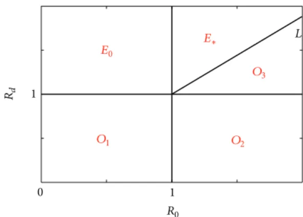
Rd R0 E0 E∗ O1 O2 O3 0 L 1 1

Figure 1:𝑅_𝑑in terms of 𝑅₀. The region of𝑂₁,𝑂₂, and𝑂₃ is the

basin of attraction of equilibrium𝑂; the region of 𝐸₀is the basin

of attraction of equilibrium𝐸₀; the region of𝐸_∗ is the basin of

attraction of equilibrium𝐸_∗; the line𝐿 is 𝑅_𝑑 = 𝑅₁ = 1 + 𝜇(𝑚 +

𝜇)(𝑚 + 𝜎)(𝑅0− 1)/𝑚𝛽(𝑚 + 𝜎 + 𝜇).

asymptotic stability theorem in [37, 38], the disease-free equilibrium point𝐸₀is globally asymptotically stable.

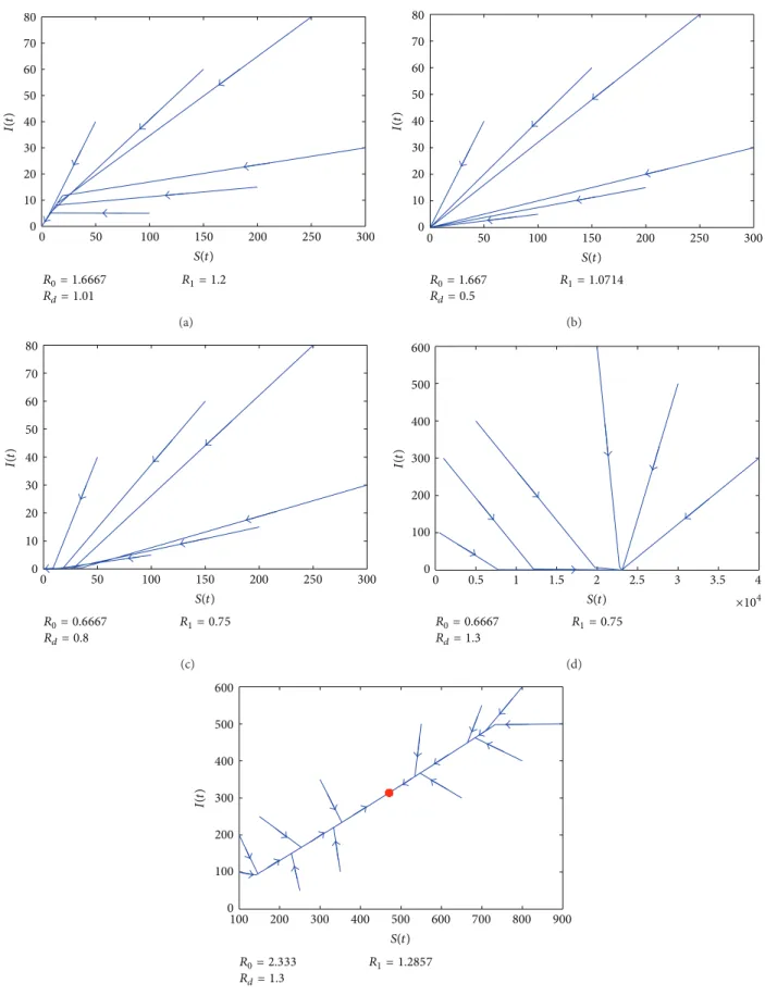
Since the proof of the stability of equilibria𝑂 and 𝐸_∗ is more difficult, we only give some numerical results.

In sum, we can show the respective basins of attraction of the three equilibria which can be seen in Figure 1 and confirmed inFigure 2.

(1) When𝑅_𝑑< 1, 𝑂 is stable; see Figures2(b)and2(c). (2) When𝑅_𝑑> 1 and 𝑅₀< 1, 𝐸₀is stable; seeFigure 2(d). (3) When𝑅_𝑑 > 1, 𝑅₀ > 1, and 𝑅_𝑑 < 𝑅₁,𝑂 is stable; see

Figure 2(a).

(4) When𝑅_𝑑> 1, 𝑅₀ > 1, and 𝑅_𝑑 > 𝑅₁,𝐸_∗is stable; see

Figure 2(e).

3. Nonautonomous Model and Analysis

3.1. The Basic Reproduction Number. Now, we consider the

non-autonomous case of the model (1) when the transmission rate is periodic, which is given as follows:

𝑑𝑆 𝑑𝑡 = 𝑟𝑁 (1 − 𝑁 𝑘) − 𝛽 (𝑡) 𝑆𝐼 𝑁 − 𝑚𝑆, 𝑑𝐸 𝑑𝑡 = 𝛽 (𝑡) 𝑆𝐼 𝑁 − 𝜎𝐸 − 𝑚𝐸, 𝑑𝐼 𝑑𝑡 = 𝜎𝐸 − 𝑚𝐼 − 𝜇𝐼, (11)

where𝛽(𝑡) is a periodic function which is proposed by [39]. In the subsequent section, we will discuss the dynamical behavior of the system (11).

For system (11), firstly we can give the basic reproduction number 𝑅₀. According to the basic reproduction number under non-autonomous system, we can refer to the method of [40,41]. From the last section, we know that system (11)

(4)

80 70 60 50 40 30 20 10 0 0 50 100 150 200 250 300 R0= 1.6667 Rd= 1.01 R1= 1.2 I(t ) S(t) (a) R0= 1.667 Rd= 0.5 R1= 1.0714 80 70 60 50 40 30 20 10 0 0 50 100 150 200 250 300 I(t ) S(t) (b) R0= 0.6667 Rd= 0.8 R1= 0.75 80 70 60 50 40 30 20 10 0 0 50 100 150 200 250 300 I(t ) S(t) (c) R0= 0.6667 Rd= 1.3 R1= 0.75 600 500 400 300 200 100 0 0 0.5 1 1.5 2 2.5 3 3.5 4 ×104 I(t ) S(t) (d) R0= 2.333 Rd= 1.3 R1= 1.2857 600 500 400 300 200 200 100 0 100 300 400 500 600 700 800 900 I(t ) S(t) (e)

Figure 2: The phase curves of the system under different initial conditions. (a) In the region𝑂₃with𝑟 = 0.101 and 𝛽 = 0.5; (b) in the region

𝑂₂with𝑟 = 0.05 and 𝛽 = 0.35; (c) in the region 𝑂₁with𝑟 = 0.08 and 𝛽 = 0.2; (d) in the region 𝐸₀with𝑟 = 0.13 and 𝛽 = 0.2; (e) in the region

(5)

has one disease-free equilibrium𝐸₀= (𝑁0, 0, 0), where 𝑁0= (1 − 𝑚/𝑟)𝑘. By giving a new vector 𝑥 = (𝐸, 𝐼), we have

𝐹 = ( 𝛽 (𝑡) 𝑆𝐼 𝑁 0 ) , 𝑉 = ( 𝑚𝐸 + 𝜎𝐸_{𝑚𝐼 + 𝜇𝐼 − 𝜎𝐸) ,} 𝑉−= (𝑚𝐸 + 𝜎𝐸_{𝑚𝐼 + 𝜇𝐼 ) ,} 𝑉+= ( 0_{𝜎𝐸) .} (12)

Taking the partial derivative of the above vectors about variables𝐸, 𝐼 and substituting the disease-free equilibrium, we have

𝐹 (𝑡) = (0 𝛽 (𝑡)_{0 0 ) ,} 𝑉 (𝑡) = (𝑚 + 𝜎_{−𝜎 𝑚 + 𝜇) .}0

(13)

According to [41], denote𝐶_𝜔to be the ordered Banach space of all 𝜔-periodic functions from R to R4 which is equipped with the maximum norm‖ ⋅ ‖ and the positive cone 𝐶+

𝜔:= {𝜙 ∈ 𝐶𝜔: 𝜙(𝑡) ≥ 0, ∀𝑡 ∈ R+}. Over the Banach space,

we define a linear operator𝐿 : 𝐶_𝜔 → 𝐶_𝜔by (𝐿𝜙) (𝑡)

= ∫∞

0 𝑌 (𝑡, 𝑡 − 𝑎) 𝐹 (𝑡 − 𝑎) 𝜙 (𝑡 − 𝑎) 𝑑𝑎, ∀𝑡 ∈ R+, 𝜙 ∈ 𝐶𝜔,

(14) where𝐿 is called the next infection operator and the inter-pretation of𝑌(𝑡, 𝑡 − 𝑎), 𝜙(𝑡 − 𝑎) can be seen in [41]. Then the spectral radius of𝐿 is defined as the basic reproduction number

𝑅₀:= 𝜌 (𝐿) . (15) In order to give the expression of the basic reproduction number, we need to introduce the linear𝜔-periodic system

𝑑𝑤

𝑑𝑡 = [−𝑉 (𝑡) +𝐹 (𝑡)𝜆 ] 𝑤, 𝑡 ∈ R+, (16) with parameter 𝜆 ∈ R. Let 𝑊(𝑡, 𝑠, 𝜆), 𝑡 ≥ 𝑠, be the evolution operator of system (16) onR2. In fact,𝑊(𝑡, 𝑠, 𝜆) =

Φ_{(𝐹/𝜆)−𝑉}(𝑡), and Φ_𝐹−𝑉(𝑡) = 𝑊(𝑡, 0, 1), for all 𝑡 ≥ 0. By

Theorems 2.1 and 2.2 in [41], the basic reproduction number also can be defined as𝜆₀such that𝜌(Φ_(𝐹/𝜆₀_)−𝑉(𝜔)) = 1, which can be straightforward to calculate.

3.2. Global Stability of the Disease-Free Equilibrium

Theorem 4. The disease-free equilibrium 𝐸₀is globally

asymp-totically stable when𝑅₀< 1 and 𝑅_𝑑> 1.

Proof. Theorem 2.2 in [41] implies that𝐸₀is locally asymp-totically stable when𝑅₀ < 1 and 𝑅_𝑑 > 1. So we only need

to prove its global attractability. It is easy to know that𝑆(𝑡) ≤ 𝑁0_{= (1 − (𝑚/𝑟))𝑘. Thus,} 𝑑𝐸 𝑑𝑡 ≤ 𝛽 (𝑡) 𝐼 − (𝑚 + 𝜎) 𝐸, 𝑑𝐼 𝑑𝑡 = 𝜎𝐸 − 𝑚𝐼 − 𝜇𝐼. (17)

The right comparison system can be written as 𝑑𝐸 𝑑𝑡 = 𝛽 (𝑡) 𝐼 − (𝑚 + 𝜎) 𝐸, 𝑑𝐼 𝑑𝑡 = 𝜎𝐸 − 𝑚𝐼 − 𝜇𝐼; (18) that is, 𝑑ℎ 𝑑𝑡 = (𝐹 (𝑡) − 𝑉 (𝑡)) ℎ (𝑡) , ℎ (𝑡) = (𝐸 (𝑡) , 𝐼 (𝑡)) . (19) For (19), Lemma 2.1 in [42] shows that there is a positive𝜔-periodic function ̂ℎ(𝑡) = (𝐸(𝑡), 𝐼(𝑡))𝑇 such that ℎ(𝑡) = 𝑒𝑝𝑡_{̂ℎ(𝑡) is a solution of system (}₁₈_{), where} _{𝑝 =}

(1/𝜔) ln 𝜌(Φ_𝐹−𝑉(𝜔)). By Theorem 2.2 in [41], we know that when𝑅₀ < 1 and 𝑅_𝑑 > 1, 𝜌(Φ_𝐹−𝑉(𝜔)) < 1 and 𝑝 < 0, which impliesℎ(𝑡) → 0 as 𝑡 → ∞. Therefore, the zero solution of system (18) is globally asymptotically stable. By the comparison principle [43] and the theory of asymptotic autonomous systems [44], when𝑅₀ < 1 and 𝑅_𝑑 > 1, 𝐸₀ is globally attractive. Therefore, the proposition that 𝐸₀ is globally asymptotically stable holds.

3.3. Existence of Positive Periodic Solutions. Before the proof

of the existence of positive periodic solutions, we firstly introduce some denotations. Let𝑢(𝑡, 𝑥₀) be the solution of system (11) with the initial value𝑥₀ = (𝑆(0), 𝐸(0), 𝐼(0)). By the fundamental existence-uniqueness theorem [45],𝑢(𝑡, 𝑥₀) is the unique solution of system (11) with𝑢(0, 𝑥₀) = 𝑥₀.

Next, we need to introduce the Poincar´e map𝑃 : 𝑋 → 𝑋 associated with system (11); that is,

𝑃 (𝑥₀) = 𝑢 (𝜔, 𝑥₀) , ∀𝑥₀∈ 𝑋, (20) where𝜔 is the period.Theorem 1implies that𝑋 is positively invariant and𝑃 is a dissipative point.

Now, we introduce two subsets of𝑋, 𝑋₀:= {(𝑆, 𝐸, 𝐼) ∈ 𝑋 : 𝐸 > 0, 𝐼 > 0} and 𝜕𝑋₀= 𝑋 \ 𝑋₀.

Lemma 5. (a) When 𝑅₀ > 1 and 𝑟 > 𝑚 + 𝜇, there exists a

𝛿 > 0 such that when

󵄩󵄩󵄩󵄩(𝑆(0),𝐸(0),𝐼(0)) − 𝐸0󵄩󵄩󵄩󵄩 ≤ 𝛿 (21)

for any(𝑆(0), 𝐸(0), 𝐼(0)) ∈ 𝑋₀, one has

lim sup

𝑚 → ∞ 𝑑 [ 𝑃

𝑚_{(𝑆 (0) , 𝐸 (0) , 𝐼 (0)) , 𝐸}

0] ≥ 𝛿, (22)

(6)

(b) When𝑅₀ > 1 and 𝑟 > 𝑚 + 𝜇, there exists a 𝛿 > 0 such that when

‖(𝑆 (0) , 𝐸 (0) , 𝐼 (0)) − 𝑂‖ ≤ 𝛿 (23)

for any(𝑆(0), 𝐸(0), 𝐼(0)) ∈ 𝑋₀, one has

lim sup

𝑚 → ∞ 𝑑 [ 𝑃

𝑚_{(𝑆 (0) , 𝐸 (0) , 𝐼 (0)) , 𝑂] ≥ 𝛿,}

(24)

where𝑂 = (0, 0, 0).

Proof. (a) By Theorem 2.2 in [41], we know that when𝑅₀> 1, 𝜌(Φ_𝐹−𝑉(𝜔)) > 1. So there is a small enough positive number 𝜖 such that 𝜌(Φ_{𝐹−𝑉−𝑀}_𝜖(𝜔)) > 1, where

𝑀_𝜖= (0

𝛽 (𝑡) 𝜖𝐼 𝑁0

0 0

) . (25)

If proposition (a) does not hold, there is some (𝑆(0), 𝐸(0), 𝐼(0)) ∈ 𝑋₀such that

lim sup

𝑚 → ∞ 𝑑 (𝑃

𝑚_{(𝑆 (0) , 𝐸 (0) , 𝐼 (0)) , 𝐸}

0) < 𝛿. (26) We can assume that for all 𝑚 ≥ 0, 𝑑(𝑃𝑚(𝑆(0), 𝐸(0), 𝐼(0)), 𝐸₀) < 𝛿. Applying the continuity of the solutions with respect to the initial values,

󵄩󵄩󵄩󵄩𝑢(𝑡,𝑃𝑚_{(𝑆 (0) , 𝐸 (0) , 𝐼 (0))) − 𝑢 (𝑡, 𝐸} 0)󵄩󵄩󵄩󵄩 ≤ 𝜖,

∀𝑚 ≥ 0, ∀𝑡1∈ [0, 𝜔] .

(27) Let𝑡 = 𝑚𝜔 + 𝑡₁, where𝑡₁ ∈ [0, 𝜔] and 𝑚 = [𝑡/𝜔]. 𝑚 = [𝑡/𝜔] is the greatest integer which is not more than 𝑡/𝜔. Then, for any𝑡 ≥ 0, 󵄩󵄩󵄩󵄩𝑢(𝑡,(𝑆(0),𝐸(0),𝐼(0))) − 𝑢(𝑡,𝐸0)󵄩󵄩󵄩󵄩 = 󵄩󵄩󵄩󵄩𝑢 (𝑡1, 𝑃𝑚(𝑆 (0) , 𝐸 (0) , 𝐼 (0))) − 𝑢 (𝑡1, 𝐸0)󵄩󵄩󵄩󵄩 ≤ 𝜖. (28) So 𝑁0 − 𝜖 ≤ 𝑆(𝑡) ≤ 𝑁0 + 𝜖. Then, when lim sup_{𝑚 → ∞}𝑑(𝑃𝑚(𝑆(0), 𝐸(0), 𝐼(0)), 𝐸₀) < 𝛿, 𝑑𝐸 𝑑𝑡 ≥ 𝛽 (𝑡) 𝐼 − 𝛽 (𝑡) 𝜖𝐼 𝑁0 − (𝑚 + 𝜎) 𝐸, 𝑑𝐼 𝑑𝑡 = 𝜎𝐸 − 𝑚𝐼 − 𝜇𝐼. (29)

Thus, we can study the right linear system 𝑑𝐸 𝑑𝑡 = 𝛽 (𝑡) 𝐼 − 𝛽 (𝑡) 𝜖𝐼 𝑁0 − (𝑚 + 𝜎) 𝐸, 𝑑𝐼 𝑑𝑡 = 𝜎𝐸 − 𝑚𝐼 − 𝜇𝐼. (30)

For the system (30), there exists a positive 𝜔-periodic function ̂𝑔(𝑡) = (𝐸(𝑡), 𝐼(𝑡))𝑇 such that𝑔(𝑡) = 𝑒𝑝𝑡̂𝑔(𝑡) is a solution of system (11), where𝑝 = (1/𝜔) ln 𝜌(Φ_{𝐹−𝑉−𝑀𝜖}(𝜔)). When𝑅₀ > 1, 𝜌(Φ_{𝐹−𝑉−𝑀𝜖}(𝜔)) > 1, which means that when

𝑔(0) > 0, 𝑔(𝑡) → ∞ as 𝑡 → ∞. By the comparison principle [43], when𝐸(0) > 0, 𝐼(0) > 0, 𝐸(𝑡) → ∞, 𝐼(𝑡) → ∞ as 𝑡 → ∞. There appears a contradiction. Thus, the proposition (a) holds.

(b) When𝑅₀> 1 and 𝑟 > 𝑚 + 𝜇, we have 𝑑𝑁 𝑑𝑡 = 𝑟𝑁 (1 − 𝑁 𝑘) − 𝑚𝑁 − 𝜇𝐼 ≥ [𝑟 (1 −𝑁 𝑘) − 𝑚 − 𝜇] 𝑁 > 0. (31)

So if𝑅_𝑑> 1, 𝑁 → 𝑁0for𝑁(0) > 0 as 𝑡 → +∞; that is, 𝑊𝑆_{(𝑂) ∩ 𝑋}

0= 0.

Theorem 6. When 𝑅₀> 1 and 𝑟 > 𝑚 + 𝜇, there exists a 𝛿 > 0

such that any solution(𝑆(𝑡), 𝐸(𝑡), 𝐼(𝑡)) of system (11) with initial

value(𝑆(0), 𝐸(0), 𝐼(0)) ∈ {(𝑆, 𝐸, 𝐼) ∈ 𝑋 : 𝐸 > 0, 𝐼 > 0} satisfies

lim inf

𝑡 → ∞ 𝐸 (𝑡) ≥ 𝛿, lim inf𝑡 → ∞ 𝐼 (𝑡) ≥ 𝛿, (32)

and system (11) has at least one positive periodic solution.

Proof. From system (11), 𝑆 (𝑡) = 𝑒− ∫0𝑡(𝛽(𝑠)𝐼(𝑠)/𝑁+𝑚)𝑑𝑠 × [𝑆 (0) + ∫𝑡 0𝑟𝑁 (𝑠) (1 − 𝑁 (𝑠) 𝑘 ) ×𝑒∫0𝑠(𝛽(𝑐)𝐼(𝑐)/𝑁(𝑐)+𝑚)𝑑𝑐𝑑𝑠] > 0, ∀𝑡 > 0, (33) 𝐸 (𝑡) = 𝑒−(𝑚+𝜎)𝑡_{[𝐸 (0) + ∫}𝑡 0 𝛽 (𝑠) 𝑆 (𝑠) 𝐼 (𝑠) 𝑁 (𝑠) 𝑒(𝑚+𝜎)𝑠𝑑𝑠] > 0, ∀𝑡 > 0, (34) 𝐼 (𝑡) = 𝑒−(𝑚+𝜇)𝑡[𝐼 (0) + ∫𝑡 0𝜎𝐸 (𝑠) 𝑒 (𝑚+𝜇)𝑠_𝑑𝑠] > 0, ∀𝑡 > 0, (35)

for any (𝑆(0), 𝐸(0), 𝐼(0)) ∈ 𝑋₀, which shows that 𝑋₀ is positively invariant. Moreover, it is obvious to see that𝜕𝑋₀ is relatively closed in𝑋. Denote

𝑀_𝜕= {(𝑆 (0) , 𝐸 (0) , 𝐼 (0)) ∈ 𝜕𝑋0 :

𝑃𝑚(𝑆 (0) , 𝐸 (0) , 𝐼 (0)) ∈ 𝜕𝑋0, ∀𝑚 ≥ 0} .

(36) Next, we prove that

𝑀_𝜕= {(𝑆, 0, 0) ∈ 𝑋 : 𝑆 ≥ 0} . (37) We only need to show that𝑀_𝜕 ⊆ {(𝑆, 0, 0) ∈ 𝑋 : 𝑆 ≥ 0}, which means that for any(𝑆(0), 𝐸(0), 𝐼(0)) ∈ 𝜕𝑋₀,𝐸(𝑚𝜔) = 𝐼(𝑚𝜔) = 0, for all 𝑚 ≥ 0. If it does not hold, there exists a𝑚₁ ≥ 0 such that (𝐸(𝑚₁𝜔), 𝐼(𝑚₁𝜔))𝑇 > 0. Taking 𝑚₁𝜔 as

(7)

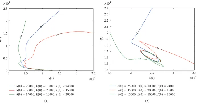
2.5 2 1.5 1 0.5 0 1 1.5 2 2.5 3 3.5 ×104 ×104 S(0) = 25000, E(0) = 10000, I(0) = 24000 S(0) = 35000, E(0) = 20000, I(0) = 15000 S(0) = 15000, E(0) = 10000, I(0) = 20000 I(t ) S(t) (a) 2.4 2.3 2.2 2.1 2 1.9 1.8 1.7 1.6 1.5 1.4 1.5 2 2.5 3 3.5 ×104 ×104 S(0) = 25000, E(0) = 10000, I(0) = 24000 S(0) = 35000, E(0) = 20000, I(0) = 15000 S(0) = 15000, E(0) = 10000, I(0) = 20000 I(t ) S(t) (b)

Figure 3: Phase plane of𝑆(𝑡) and 𝐼(𝑡). (a) When the parameter values are 𝑟 = 0.13, 𝑎 = 0.3, and 𝑏 = 0.2, 𝑅₀ = 0.9029 < 1, 𝑅_𝑑= 1.3 > 1. (b)

When the parameter values are𝑟 = 0.3, 𝑎 = 0.7, and 𝑏 = 0.2, 𝑅₀= 2.1067 and 𝑟 > 𝑚 + 𝜇. The value of other parameters can be seen inTable 1.

the initial time and repeating the processes as in (33)–(35), we can have that (𝑆(𝑡), 𝐸(𝑡), 𝐼(𝑡))𝑇 > 0, for all 𝑡 > 𝑚₁𝜔. Thus,(𝑆(𝑡), 𝐸(𝑡), 𝐼(𝑡)) ∈ 𝑋₀, for all𝑡 > 𝑚₁𝜔. There appears a contradiction, which means that the equality (37) holds. Therefore,𝐸₀is acyclic in𝜕𝑋₀. Obviously, when𝑅₀ > 1 and 𝑟 > 𝑚 + 𝜇, 𝑂 is acyclic in 𝜕𝑋₀.

Furthermore, by Lemma 5, 𝐸₀ = (𝑁0, 0, 0) and 𝑂 = (0, 0, 0) are isolated invariant sets in 𝑋, 𝑊𝑆_(𝐸

0) ∩ 𝑋0 = 0,

and𝑊𝑆(𝑂) ∩ 𝑋₀ = 0. By Theorem 1.3.1 and Remark 1.3.1 in [46], it can be obtained that𝑃 is uniformly persistent with respect to(𝑋₀, 𝜕𝑋₀); that is, there exists a 𝛿 > 0 such that any solution(𝑆(𝑡), 𝐸(𝑡), 𝐼(𝑡)) of system (11) with the initial value (𝑆(0), 𝐸(0), 𝐼(0)) ∈ {(𝑆, 𝐸, 𝐼) ∈ 𝑋 : 𝐸 > 0, 𝐼 > 0} satisfies

lim inf

𝑡 → ∞ 𝐸 (𝑡) ≥ 𝛿, lim inf𝑡 → ∞ 𝐼 (𝑡) ≥ 𝛿. (38)

Applying Theorem1.3.6 in [46],𝑃 has a fixed point (𝑆∗(0) , 𝐸∗(0) , 𝐼∗(0)) ∈ 𝑋₀. (39) From (33), we know𝑆∗ > 0, for all 𝑡 ∈ [0, 𝜔]. 𝑆∗(𝑡) is also more than zero for all𝑡 > 0 due to the periodicity. Similarly, for all𝑡 ≥ 0, 𝐸∗(𝑡) > 0, 𝐼∗(𝑡) > 0. Therefore, it can be obtained that one of the positive𝜔-periodic solutions of system (11) is (𝑆∗(𝑡), 𝐸∗(𝑡), 𝐼∗(𝑡)).

3.4. Numerical Simulations. Firstly, we give some notations.

If𝑔(𝑡) is a periodic function with period 𝜔, we define 𝑔 = (1/𝜔) ∫₀𝜔𝑔(𝑡)𝑑𝑡, 𝑔𝑙 _{= min}

𝑡∈[0,𝜔]𝑔(𝑡), 𝑔𝑢 = max𝑡∈[0,𝜔]𝑔(𝑡). As

described in the previous section,

𝑅₁(𝑡) = 1 +𝜇 (𝑚 + 𝜇) (𝑚 + 𝜎) (𝑅0− 1)

𝑚𝛽 (𝑡) (𝑚 + 𝜎 + 𝜇) . (40)

So𝑅𝑙₁= 1 + 𝜇(𝑚 + 𝜇)(𝑚 + 𝜎)(𝑅𝑙₀− 1)/𝑚𝛽𝑢(𝑚 + 𝜎 + 𝜇), 𝑅𝑢₁= 1 + 𝜇(𝑚 + 𝜇)(𝑚 + 𝜎)(𝑅𝑢

0− 1)/𝑚𝛽𝑙(𝑚 + 𝜎 + 𝜇).

In this section, we adopt 𝛽(𝑡) = 𝑎[1 + 𝑏 sin(𝜋𝑡/10)]. Then, applying the numerical simulation to verify the above solution, we give the following conclusion:

(1) when𝑅_𝑑< 1, 𝑂 is stable;

(2) when𝑅_𝑑> 1 and 𝑅₀< 1, 𝐸₀is stable; seeFigure 3(a); (3) when𝑅₀ > 1 and 𝑟 > 𝑚 + 𝜇, system (11) has at least

one positive periodic solution; seeFigure 3(b). We can give more results about the conditions of existence of the positive periodic solution.

(1󸀠) When 𝑅𝑑 > 1, 𝑅0 > 1, and 𝑅𝑑 < 𝑅𝑢1,𝑂 is stable; see

Figures4(a)and4(b). (2󸀠_{) When 𝑅}

𝑑> 1, 𝑅0> 1, and 𝑅𝑑> 𝑅𝑢1, system (11) has at

least one positive periodic solution, seeFigure 5. By numerical simulations, we can give that the conditions which ensure the existence of positive periodic solution are 𝑅₀> 1 and 𝑟 > 𝑚 + 𝜇 or 𝑅_𝑑> 1, 𝑅₀> 1, and 𝑅_𝑑> 𝑅𝑢

1. In fact,

𝑅_𝑑> 1, 𝑅₀> 1, and 𝑅_𝑑> 𝑅𝑢

1are the sufficient conditions for

𝑅₀> 1 and 𝑟 > 𝑚 + 𝜇. As a result, the conditions 𝑅₀> 1 and 𝑟 > 𝑚 + 𝜇 are broader.

4. Discussion

This paper considers a logistic growth system whose birth process incorporates density-dependent effects. This type of model has a rich dynamical behavior and practical signif-icance. By analyzing its equilibria and respective attractive region, we find that the dynamical behavior of a disease will

(8)

2.5 2 1.5 1 0.5 0 0 0.5 1 1.5 2 2.5 3 3.5 ×104 ×104 S(0) = 25000, E(0) = 10000, I(0) = 24000 S(0) = 35000, E(0) = 20000, I(0) = 15000 S(0) = 15000, E(0) = 10000, I(0) = 20000 I(t ) S(t) (a) 2.5 2 1.5 1 0.5 0 0 0.5 1 1.5 2 2.5 3 3.5 ×104 ×104 S(0) = 25000, E(0) = 10000, I(0) = 24000 S(0) = 35000, E(0) = 20000, I(0) = 15000 S(0) = 15000, E(0) = 10000, I(0) = 20000 I(t ) S(t) (b)

Figure 4: Phase plane of𝑆(𝑡) and 𝐼(𝑡). (a) When the parameter values are 𝑟 = 0.11, 𝑎 = 0.9, 𝑏 = 0.2 and 𝜇 = 0.3, 𝑅₀= 1.4991, 𝑅_𝑑= 1.1 > 1,

𝑅𝑑 < 𝑅𝑢1 = 1.4159, and 𝑅𝑑 < 𝑅𝑙1 = 1.2773. (b) When the parameter values are 𝑟 = 0.126, 𝑎 = 0.7, 𝑏 = 0.2, and 𝜇 = 0.3, 𝑅0 = 2.1067,

𝑅_𝑑= 1.26 > 1, 𝑅_𝑑< 𝑅𝑢

1= 1.2964, and 𝑅𝑑> 𝑅𝑙1= 1.1976. The value of other parameters can be seen inTable 1.

7000 6000 5000 4000 3000 2000 1000 0 0.5 1 1.5 2 ×104 ×104 S(0) = 22000, E(0) = 5000, I(0) = 1000 S(0) = 4000, E(0) = 2000, I(0) = 1000 S(0) = 10000, E(0) = 10000, I(0) = 6000 I(t ) S(t)

Figure 5: Phase plane of𝑆(𝑡) and 𝐼(𝑡). When the parameter values

are𝑟 = 0.13, 𝑎 = 0.36, and 𝑏 = 0.2, 𝑅₀= 1.0834, 𝑅_𝑑= 1.3 > 1, 𝑅_𝑑>

𝑅𝑢

1 = 1.0435, and 𝑅𝑑 > 𝑅𝑙1 = 1.029. The value of other parameters

can be seen inTable 1.

be determined by two thresholds𝑅₀ and𝑅_𝑑. Only𝑅₀ > 1 cannot promise the existence of the endemic equilibrium which also needs𝑅_𝑑 > 𝑅₁. When 𝑅₀ > 1 and 𝑅_𝑑 < 𝑅₁, the solutions of the system (1) will tend to the origin𝑂. It

is caused by the phenomenon that the death number due to disease cannot be supplemented by the birth number promptly. Finally, all people are infected and die out. The fact interpreted by this model is more reasonable. Theoretically, we prove the global asymptotic stability of the disease-free equilibrium and give respective attractive regions of equilibria.

Seasonally effective contact rate is the most common form which may be related to various factors, and thus this paper studies the corresponding non-autonomous system which is obtained by changing the constant transmission rate of the above system into the periodic transmission rate. For the periodic systems, their dynamical behaviors, especially the basic reproduction number, have been investigated in depth by [41, 47–55] which provide many methods that we can utilize. For the obtained periodic model, by analyzing the global asymptotic stability of the disease-free equilibrium and the existence of positive periodic solution, we have the similar results as the autonomous system. The dynamic behavior of disease will be decided by two conditions𝑅₀ > 1 and 𝑟 > 𝑚 + 𝜇 that show that when the disease is prevalent, the birth rate should be larger than the death rate to guarantee the sustainable growth of population. Otherwise, the population will disappear. In addition, we will evaluate and compare the basic reproduction number 𝑅₀ and the average basic reproduction number𝑅₀which has been adopted by [27,56–

59]. In this paper, we can calculate the average reproduction number

𝑅₀= 𝛽𝜎

(9)

where𝛽 = (1/20) ∫₀20𝛽(𝑡)𝑑𝑡. When 𝑟 = 0.13, 𝑎 = 0.3, and 𝑏 = 0.2, we know that 𝑅₀ = 0.9029 and 𝑅₀ = 1. When 𝑟 = 0.13, 𝑘 = 100000, 𝑎 = 0.36, 𝑏 = 0.2, and 𝑚 = 0.1, 𝜎 = 0.2, 𝜇 = 0.1, then 𝑅₀ = 1.0834 and 𝑅₀ = 1.2. In that sense, it is confirmed that the basic reproduction number𝑅₀defined by [40] is more accurate than the average reproduction number 𝑅₀which overestimates the risk of disease.

It should be noted that we live in a spatial world and it is a natural phenomenon that a substance goes from high density regions to low density regions. As a result, epidemic models should include spatial effects. In a further study, we need to investigate spatial epidemic models with seasonal factors.

Acknowledgments

The research was partially supported by the National Natural Science Foundation of China under Grant nos. 11301490, 11301491, 11331009, 11147015, 11171314, 11101251, and 11105024, Natural Science Foundation of ShanXi Province Grant no. 2012021002-1, and the Opening Foundation of Institute of Information Economy, Hangzhou Normal University, Grant no. PD12001003002003.

References

[1] K. Dietz and J. A. P. Heesterbeek, “Bernoulli was ahead of modern epidemiology,” Nature, vol. 408, no. 6812, pp. 513–514, 2000.

[2] K. Dietz and J. A. P. Heesterbeek, “Daniel Bernoulli’s epidemio-logical model revisited,” Mathematical Biosciences, vol. 180, pp. 1–21, 2002.

[3] R. Ross, “An application of the theory of probabilities to the study of a priori pathometry (part I),” Proceedings of the Royal

Society A, vol. 92, no. 638, pp. 204–230, 1916.

[4] R. Ross and H. P. Hudson, “An application of the theory of probabilities to the study of a priori pathometry (part II),”

Proceedings of the Royal Society A, vol. 93, no. 650, pp. 212–225,

1917.

[5] W. O. Kermack and A. G. McKendrick, “A contribution to the mathematical theory of epidemics (part I),” Proceedings of the

Royal Society A, vol. 115, no. 772, pp. 700–721, 1927.

[6] W. O. Kermack and A. G. McKendrick, “A contribution to the mathematical theory of epidemics (part II),” Proceedings of the

Royal Society A, vol. 138, no. 834, pp. 55–83, 1932.

[7] A. Tsoularis and J. Wallace, “Analysis of logistic growth models,”

Mathematical Biosciences, vol. 179, no. 1, pp. 21–55, 2002.

[8] I. N˚asell, “On the quasi-stationary distribution of the stochastic logistic epidemic,” Mathematical Biosciences, vol. 156, no. 1-2, pp. 21–40, 1999.

[9] H. Fujikawa, A. Kai, and S. Morozumi, “A new logistic model for

Escherichia coli growth at constant and dynamic temperatures,” Food Microbiology, vol. 21, no. 5, pp. 501–509, 2004.

[10] L. Berezansky and E. Braverman, “Oscillation properties of a logistic equation with several delays,” Journal of Mathematical

Analysis and Applications, vol. 247, no. 1, pp. 110–125, 2000.

[11] M. Tabata, N. Eshima, and I. Takagi, “The nonlinear integro-partial differential equation describing the logistic growth of human population with migration,” Applied Mathematics and

Computation, vol. 98, pp. 169–183, 1999.

[12] L. Korobenko and E. Braverman, “On logistic models with a car-rying capacity dependent diffusion: stability of equilibria and coexistence with a regularly diffusing population,” Nonlinear

Analysis: Real World Applications, vol. 13, no. 6, pp. 2648–2658,

2012.

[13] Y. Muroya, “Global attractivity for discrete models of nonau-tonomous logistic equations,” Computers and Mathematics with

Applications, vol. 53, no. 7, pp. 1059–1073, 2007.

[14] S. Invernizzi and K. Terpin, “A generalized logistic model for photosynthetic growth,” Ecological Modelling, vol. 94, no. 2-3, pp. 231–242, 1997.

[15] Z. Min, W. Bang-Jun, and J. Feng, “Coalmining cities’ economic growth mechanism and sustainable development analysis based on logistic dynamics model,” Procedia Earth and Planetary

Science, vol. 1, no. 1, pp. 1737–1743, 2009.

[16] L. I. Anit¸a, S. Anit¸a, and V. Arnˇautu, “Global behavior for an age-dependent population model with logistic term and periodic vital rates,” Applied Mathematics and Computation, vol. 206, no. 1, pp. 368–379, 2008.

[17] Z. A. Banaszak, X. Q. Tang, S. C. Wang, and M. B. Zaremba, “Logistics models in flexible manufacturing,” Computers in

Industry, vol. 43, no. 3, pp. 237–248, 2000.

[18] S. Brianzoni, C. Mammana, and E. Michetti, “Nonlinear dynamics in a business-cycle model with logistic population growth,” Chaos, Solitons and Fractals, vol. 40, no. 2, pp. 717–730, 2009.

[19] W. P. London and J. A. Yorke, “Recurrent outbreaks of measles, chickenpox and mumps. I. Seasonal variation in contact rates,”

The American Journal of Epidemiology, vol. 98, no. 6, pp. 453–

468, 1973.

[20] S. F. Dowell, “Seasonal variation in host susceptibility and cycles of certain infectious diseases,” Emerging Infectious Diseases, vol. 7, no. 3, pp. 369–374, 2001.

[21] O. N. Bjørnstad, B. F. Finkenst¨adt, and B. T. Grenfell, “Dynamics of measles epidemics: estimating scaling of transmission rates using a Time series SIR model,” Ecological Monographs, vol. 72, no. 2, pp. 169–184, 2002.

[22] J. Zhang, Z. Jin, G. Q. Sun, X. Sun, and S. Ruan, “Modeling seasonal rabies epidemics in China,” Bulletin of Mathematical

Biology, vol. 74, no. 5, pp. 1226–1251, 2012.

[23] I. B. Schwartz, “Small amplitude, long period outbreaks in seasonally driven epidemics,” Journal of Mathematical Biology, vol. 30, no. 5, pp. 473–491, 1992.

[24] I. B. Schwartz and H. L. Smith, “Infinite subharmonic bifur-cation in an SEIR epidemic model,” Journal of Mathematical

Biology, vol. 18, no. 3, pp. 233–253, 1983.

[25] H. L. Smith, “Multiple stable subharmonics for a periodic epidemic model,” Journal of Mathematical Biology, vol. 17, no. 2, pp. 179–190, 1983.

[26] J. Dushoff, J. B. Plotkin, S. A. Levin, and D. J. D. Earn, “Dynamical resonance can account for seasonality of influenza epidemics,” Proceedings of the National Academy of Sciences of

the United States of America, vol. 101, no. 48, pp. 16915–16916,

2004.

[27] J. L. Ma and Z. Ma, “Epidemic threshold conditions for seasonally forced SEIR models,” Mathematical Biosciences and

Engineering, vol. 3, no. 1, pp. 161–172, 2006.

[28] D. J. D. Earn, P. Rohani, B. M. Bolker, and B. T. Grenfell, “A simple model for complex dynamical transitions in epidemics,”

(10)

[29] M. J. Keeling, P. Rohani, and B. T. Grenfell, “Seasonally forced disease dynamics explored as switching between attractors,”

Physica D, vol. 148, no. 3-4, pp. 317–335, 2001.

[30] J. L. Aron and I. B. Schwartz, “Seasonality and period-doubling bifurcations in an epidemic model,” Journal of Theoretical

Biology, vol. 110, no. 4, pp. 665–679, 1984.

[31] N. C. Grassly and C. Fraser, “Seasonal infectious disease epidemiology,” Proceedings of the Royal Society B, vol. 273, no. 1600, pp. 2541–2550, 2006.

[32] J. Zhang, Z. Jin, G. Q. Sun, T. Zhou, and S. Ruan, “Analysis of rabies in China: transmission dynamics and control,” PLoS

ONE, vol. 6, no. 7, Article ID e20891, 2011.

[33] O. Diekmann, J. A. P. Heesterbeek, and J. A. Metz, “On the definition and the computation of the basic reproduction

ratio R₀ in models for infectious diseases in heterogeneous

populations,” Journal of mathematical biology, vol. 28, no. 4, pp. 365–382, 1990.

[34] O. Diekmann, J. A. P. Heesterbeek, and M. G. Roberts, “The construction of next-generation matrices for compartmental epidemic models,” Journal of the Royal Society Interface, vol. 7, no. 47, pp. 873–885, 2010.

[35] P. van den Driessche and J. Watmough, “Reproduction numbers and sub-threshold endemic equilibria for compartmental mod-els of disease transmission,” Mathematical Biosciences, vol. 180, pp. 29–48, 2002.

[36] F. Berezovsky, G. Karev, B. J. Song, and C. C. Chavez, “A simple epidemic model with surprising dynamics,” Mathematical

Bio-sciences and Engineering, vol. 2, pp. 133–152, 2005.

[37] J. LaSalle and S. Lefschetz, Stability by Liapunov’s Direct Method, Academic Press, New York, NY, USA, 1961.

[38] E. A. Barbashin, Introduction to the Theory of Stability, Wolters-Noordhoff, Groningen, The Netherlands, 1970.

[39] D. Schenzle, “An age-structured model of pre- and post-vaccination measles transmission,” Mathematical Medicine and

Biology, vol. 1, no. 2, pp. 169–191, 1984.

[40] N. Baca¨er and S. Guernaoui, “The epidemic threshold of vector-borne diseases with seasonality: the case of cutaneous leishmaniasis in Chichaoua, Morocco,” Journal of Mathematical

Biology, vol. 53, no. 3, pp. 421–436, 2006.

[41] W. D. Wang and X. Q. Zhao, “Threshold dynamics for compart-mental epidemic models in periodic environments,” Journal of

Dynamics and Differential Equations, vol. 20, no. 3, pp. 699–717,

2008.

[42] F. Zhang and X. Q. Zhao, “A periodic epidemic model in a patchy environment,” Journal of Mathematical Analysis and

Applications, vol. 325, no. 1, pp. 496–516, 2007.

[43] H. L. Smith and P. Waltman, The Theory of the Chemostat, Cambridge University Press, New York, NY, USA, 1995. [44] H. R. Thieme, “Convergence results and a Poincar´e-Bendixson

trichotomy for asymptotically automous differential equations,”

Journal of Mathematical Biology, vol. 30, pp. 755–763, 1992.

[45] L. Perko, Differential Equations and Dynamical Systems, Springer, New York, NY, USA, 2000.

[46] X. Q. Zhao, Dynamical Systems in Population Biology, Springer, New York, NY, USA, 2003.

[47] Z. G. Bai and Y. C. Zhou, “Threshold dynamics of a bacillary dysentery model with seasonal fluctuation,” Discrete and

Con-tinuous Dynamical Systems B, vol. 15, no. 1, pp. 1–14, 2011.

[48] Z. G. Bai, Y. C. Zhou, and T. L. Zhang, “Existence of multiple periodic solutions for an SIR model with seasonality,” Nonlinear

Analysis: Theory, Methods and Applications, vol. 74, no. 11, pp.

3548–3555, 2011.

[49] N. Baca¨er, “Approximation of the basic reproduction number

R₀for vector-borne diseases with a periodic vector population,”

Bulletin of Mathematical Biology, vol. 69, no. 3, pp. 1067–1091,

2007.

[50] N. Baca¨er and X. Abdurahman, “Resonance of the epidemic threshold in a periodic environment,” Journal of Mathematical

Biology, vol. 57, no. 5, pp. 649–673, 2008.

[51] N. Baca¨er, “Periodic matrix population models: growth rate, basic reproduction number, and entropy,” Bulletin of

Mathemat-ical Biology, vol. 71, no. 7, pp. 1781–1792, 2009.

[52] N. Baca¨er and E. H. A. Dads, “Genealogy with seasonality, the basic reproduction number, and the influenza pandemic,”

Journal of Mathematical Biology, vol. 62, no. 5, pp. 741–762, 2011.

[53] L. J. Liu, X. Q. Zhao, and Y. C. Zhou, “A tuberculosis model with seasonality,” Bulletin of Mathematical Biology, vol. 72, no. 4, pp. 931–952, 2010.

[54] J. L. Liu, “Threshold dynamics for a HFMD epidemic model with periodic transmission rate,” Nonlinear Dynamics, vol. 64, no. 1-2, pp. 89–95, 2011.

[55] Y. Nakata and T. Kuniya, “Global dynamics of a class of SEIRS epidemic models in a periodic environment,” Journal of

Mathematical Analysis and Applications, vol. 363, no. 1, pp. 230–

237, 2010.

[56] B. G. Williams and C. Dye, “Infectious disease persistence when transmission varies seasonally,” Mathematical Biosciences, vol. 145, no. 1, pp. 77–88, 1997.

[57] I. A. Moneim, “The effect of using different types of periodic contact rate on the behaviour of infectious diseases: a simula-tion study,” Computers in Biology and Medicine, vol. 37, no. 11, pp. 1582–1590, 2007.

[58] C. L. Wesley and L. J. S. Allen, “The basic reproduction number in epidemic models with periodic demographics,” Journal of

Biological Dynamics, vol. 3, no. 2-3, pp. 116–129, 2009.

[59] D. Greenhalgh and I. A. Moneim, “SIRS epidemic model and simulations using different types of seasonal contact rate,”

Systems Analysis Modelling Simulation, vol. 43, no. 5, pp. 573–

(11)

Submit your manuscripts at

http://www.hindawi.com

Hindawi Publishing Corporation

http://www.hindawi.com Volume 2014

Mathematics

Journal of

http://www.hindawi.com Volume 2014 Mathematical Problems in Engineering

Hindawi Publishing Corporation http://www.hindawi.com Differential Equations International Journal of Volume 2014

Journal of

Applied Mathematics

Probability

and

Statistics

http://www.hindawi.com Volume 2014 Advances in

Mathematical Physics

Complex Analysis

Journal of

Optimization

Journal of

International Journal of

Combinatorics

Operations

Research

Journal of Function Spaces

Abstract and Applied Analysis

http://www.hindawi.com Volume 2014 International Journal of Mathematics and Mathematical Sciences

Positive periodic solutions of an epidemic model with seasonality

Research Article