How Macroeconomists Lost Control of Stabilization Policy: Towards Dark Ages

HAL Id: halshs-02978527

https://halshs.archives-ouvertes.fr/halshs-02978527

HAL is a multi-disciplinary open access archive for the deposit and dissemination of sci-entific research documents, whether they are pub-lished or not. The documents may come from teaching and research institutions in France or abroad, or from public or private research centers.

L’archive ouverte pluridisciplinaire HAL, est destinée au dépôt et à la diffusion de documents scientifiques de niveau recherche, publiés ou non, émanant des établissements d’enseignement et de recherche français ou étrangers, des laboratoires publics ou privés.

How Macroeconomists Lost Control of Stabilization

Policy: Towards Dark Ages

Jean-Bernard Chatelain, Kirsten Ralf

To cite this version:

Jean-Bernard Chatelain, Kirsten Ralf. How Macroeconomists Lost Control of Stabilization Policy: Towards Dark Ages. 2020. �halshs-02978527�

WORKING PAPER N° 2020 – 60

How Macroeconomists Lost Control of Stabilization Policy:

Towards Dark Ages

Jean-Bernard Chatelain

Kirsten Ralf

JEL Codes: C61, C62, E43, E44, E47, E52, E58

Keywords: Control, Stabilization Policy Ine¤ectiveness, Negative feedback, Dynamic Games

How Macroeconomists Lost Control of

Stabilization Policy: Towards Dark Ages

Jean-Bernard Chatelain

and Kirsten Ralf

September 25, 2020

Abstract

This paper is a study of the history of the transplant of mathematical tools using negative feedback for macroeconomic stabilization policy from 1948 to 1975 and the subsequent break of the use of control for stabilization policy which occurred from 1975 to 1993. New-classical macroeconomists selected a subset of the tools of control that favored their support of rules against discretionary stabilization policy. The Lucas critique and Kydland and Prescott’s time-inconsistency were over-statements that led to the “dark ages" of the prevalence of the stabilization-policy-ine¤ectiveness idea. These over-statements were later revised following the success of the Taylor (1993) rule.

JEL classi…cation numbers: C61, C62, E43, E44, E47, E52, E58.

Keywords: Control, Stabilization Policy Ine¤ectiveness, Negative feedback, Dynamic Games.

1

Introduction

This paper presents a longitudinal study of the transplant of key ideas and mathematical tools from negative-feedback control in engineering and applied mathematics to macro-economic stabilization policy. This movement evolved parallel to the “rules versus discre-tion”or “stabilization policy ine¤ectiveness”controversy from 1948 to 1993. In particular, we observe a fast transplant of classic control and optimal control to stabilization pol-icy in the 1950s and 1960s, followed by a long delay to transplant robust control and stochastic optimal control to optimal state estimation and optimal policy. The paper re-evaluates the Lucas critique and time-inconsistency argument which contributed to the bifurcation with diverging paths between control versus the modeling of stabilization policy by mainstream macroeconomics in the 1970s and 1980s.

Adam Smith (1776) believed that demand and supply are always self stabilizing due to a negative feedback mechanism in the private sector. In the 1930s emerged Keynesian

We thank two anonymous referees and editors Hans Michael Trautwein André Lapidus, Jean-Sébastien Lenfant and Goulven Rubin. We thank Alain Raybaut our discussant as well as participants of the session at ESHET conference in Lille 2019. We thank Marwan Simaan and Edward Nelson for useful comments.

y_{Paris School of Economics, Université Paris I Pantheon Sorbonne, 48 Boulevard Jourdan 75014 Paris.} Email: jean-bernard.chatelain@univ-paris1.fr.

z_{ESCE International Business School, INSEEC U. Research Center, 10 rue Sextius Michel, 75015} Paris, Email: Kirsten.Ralf@esce.fr

macroeconomic stabilization policy where the policy maker uses negative feedback mech-anisms with monetary or …scal policy instruments. Friedman (1948) started the rules versus discretion controversy, when he proposed …scal rules that do not vary in response to cyclical ‡uctuations in business activity, so that it is the private sector’s negative-feedback mechanism that stabilizes the economy, and not the policy maker. He de…ned “discretion” as Keynesian state contingent policy where the policy instruments change with respect to the deviation of policy targets from their set points. Discretionary policy was used in the US in the 1950s and 1960s, and the proponents of rules were losing in the controversy during these two decades.

In parallel to the development of Keynesian stabilization policy, the …eld of applied mathematics and engineering developed the tools of classic control during 1930-1955 (Ben-nett (1996)). This …eld gains maturity and autonomy while creating a world association with a …rst IFAC conference in 1960. Between 1955 and 1990, it has an impressive and fast rate of new discoveries: optimal control, optimal state estimation with Kalman …lter, stochastic optimal control, robust optimal control, Nash and Stackelberg dynamic games. These discoveries were readily applied for many devices with numerical algorithms using the development of computers at the time. Aström and Kumar (2014) survey the research …eld of control which is based on negative-feedback rules stabilizing a dynamic system:

Feedback is an ancient idea, but feedback control is a young …eld... Its development as a …eld involved contributions from engineers, mathematicians, economists and physicists. It represented a paradigm shift because it cut across the traditional engineering disciplines of aeronautical, chemical, civil, electrical and mechanical engineering, as well as economics and operations research. The scope of control makes it the quintessential multidisciplinary …eld. (Aström and Kumar (2014), p. 3)

There was a strong demand for control tools for …rm-level planning and for macroeco-nomic stabilization policy in the 1960s (Kendrick (1976), Kendrick (2005), Neck (2009)

and Turnovsky (2011)). Barnett describes the related controversies surrounding the

model of the Federal Reserve Board in the 1970s (Barnett and Serletis (2017)): The policy simulations were collected together to display the policy target paths that would result from various choices of instrument paths. The model was very large, with hundreds of equations. Some economists advocated re-placing the “menu” book of simulations with a single recommended policy, produced by applying optimal control theory to the model. The model was called the FMP model, for Federal Reserve-MIT-Penn, since the origins of the model were with work done by Franco Modigliani at MIT and Albert Ando at the U. of Pennsylvania, among others. That model’s simulations subsequently became an object of criticism by advocates of the Lucas Critique. The alter-native optimal control approach became an object of criticism by advocates of the Kydland and Prescott (1977) …nding of time inconsistency of optimal control policy. (Barnett and Serletis (2017), p. 7-8)

The Lucas (1976) critique and Kydland and Prescott’s (1977) time-inconsistency argu-ment convinced a su¢ cient number of macroeconomists that, although negative-feedback mechanism and optimal control should be used for modeling the private sector, negative-feedback mechanism and optimal control cannot be used for stabilization policy by macro-economists and practitioners of monetary and …scal policy.

In the 1970s, Lucas, Kydland and Prescott, labeled as new classical macroeconomists, took sides for rules in the rules versus discretion controversy. On the one hand, incor-porating control tools into macroeconomics was obviously a scienti…c progress, and new classical macroeconomists invested heavily, like Keynesian macroeconomists, in learning these tools in the 1960s. On the other hand, control tools were supporting negative-feedback mechanism driven by policy makers, hence discretion. Therefore, the tools of control were pivotal in the rules versus discretion controversy.

E¢ cient multi-disciplinary research tools can be imported from one …eld of research to another one. However, the scientists in the …eld of arrival are free to bias their choice of the tools to be imported from the …eld of origin, if they are taking side in a scienti…c controversy. This selection bias entails the risk of the inconsistency of the imported subset of tools with respect to the …eld of origin.

The new-classical economists put forward their normative rational expectations theory with theoretical demonstrations using a Kalman …lter. They claimed it is impossible to estimate parameters of the transmission mechanism when there is reverse causality of the feedback rule. The new-classical economists suggested importing time-inconsistency into dynamic games. They simulated models using the linear quadratic regulator for the private sector. All these approaches are using tools from the …eld of control.

But, in addition, following the complete guidelines of the …eld of control where the accuracy of the measurement of the transmission mechanism is a key element, they could have attempted the falsi…cation of their theory estimating parameters with a Kalman …lter. They could have attempted to devote a lot of resources to identi…cation strategies when facing reverse causality in systems of equations. They could have determined opti-mal feedback policy based on these estimation of state variables using stochastic optiopti-mal control. They could have searched for a policy that could be robust to some ranges of uncertainty on parameters of the transmission mechanism.

But using these tools would have been inconsistent with their research agenda where they were taking sides in a scienti…c controversy. They biased the use of some tools of control in order to support their prior view on the side of “rules”in the controversy. The temporary success (for two decades) of their selection bias restricted the demand and delayed the use of the tools of control for stabilization policy.

This helps to reconsider how, in order to convince a su¢ ciently large subset of the community of macroeconomists, the authors rhetorically generalized some valid state-ments of their papers stretching them to extreme conclusions, which, in turn, were false statements.

The Lucas critique (1976) over-stated that it is impossible to identify parameters in a dynamic system of equations with reverse causality. Despite the Lucas critique, Kydland and Prescott (1982) over-stated that the US economy during 1950-1979 behaved as if stabilization policy had never been implemented (policy instruments were pegged) or as if the policy instruments did not have an e¤ect on policy targets. Kydland and Prescott (1977) over-stated that policy maker’s credibility can never be achieved using negative-feedback rules according to optimal control.

Simulations using private sector micro-economic foundations and auto-regressive ex-ogenous shocks were rhetorically presented as the magical “scienti…c”solution to answer the Lucas critique, to avoid time inconsistency and to describe business cycles data.

These rhetorics marginalized or delayed for at least a decade attempts to model sta-bilization policy transplanting the new tools of robust optimal control facing parameter uncertainty and stochastic optimal control with feedback rules reacting to estimates of

state variables using a Kalman …lter with macroeconomic time-series. This outcome is labeled “dark ages” by Taylor (2007):

But after this ‡urry of work in the late 1970s and early 1980s, a sort of “dark age” for this type of modeling began to set in. Ben McCallum (1999) discussed this phenomenon in his review lecture, and from the perspective of the history of economic thought, it is an interesting phenomenon. As he put it, there was “a long period during which there was a great falling o¤ in the volume of sophisticated yet practical monetary policy analysis". (Taylor (2007))

In order to explain the selection of tools imported from control on behalf of the new-classical macroeconomist side in the “rules versus discretion”controversy, our method is to use as a reference model the simplest model of control. We translate the mathematical arguments of the most cited papers in this controversy into the framework of this single model. This helps to understand how di¤erent de…nitions of discretion and how di¤erent hypothesis on the persistence of the policy targets in the transmission mechanism matter, even though they were not highlighted so far in the history of the rules versus discretion controversy.

The structure of this study is as follows:

Section 2 frames the original classical economists’view of self-stabilizing markets in the framework of Ezekiel’s (1938) Cobweb model. Friedman’s (1948) and Kydland and Prescott’s (1977) rules versus discretion controversy is presented in the framework of the simplest …rst order single-input single-output model of control.

Section 3 documents the fast transplant of classic control from Phillips (1954b) and resurrection with the Taylor (1993) rule. It mentions the fast transplant of optimal con-trol to stabilization policy in the 1960s and of a Kalman …lter for rational expectations theory. By contrast, It mentions the very limited use of Stochastic Optimal Control us-ing simultaneously Kalman-…lter estimations for determinus-ing optimal stabilization policy in the linear quadratic Gaussian model. Finally, it emphasizes the long delay before transplanting robust control, dealing with the uncertainty on parameters.

Section 4 re-evaluates the claim of the Lucas (1976) critique that it is impossible to identify the parameters of the transmission mechanism when there is reverse causality due to a negative-feedback rule. The Lucas critique is not resolved by microeconomic foundations, by Sims’ (1980) vector autoregressive models, by Kydland and Prescott’s (1982) real business cycle, nor by Lucas’(1987) welfare cost of business cycles. Kydland and Prescott (1977) section 5 has a speci…c de…nition of discretion assuming a Lucas critique bias, which is not related to time-inconsistency.

Section 5 re-evaluates the time-inconsistency argument and the impossibility of pol-icy maker’s credibility leading to the impossibility to use negative feedback grounded by control. Firstly, it credits time-inconsistency to Simaan and Cruz’ (1973b) …rst contri-bution with Kydland (1975, 1977), Calvo (1978) and Kydland and Prescott (1980) as followers. Secondly, it highlights that the in‡ationary bias in Barro and Gordon’s (1983) static model is distinct from Calvo’s (1978) dynamic time-inconsistency.

Section 6 explains how Taylor (1993) rhetorically translated Friedman’s (1948) rules versus discretion controversy in his “Semantics”section to the advantage of the negative-feedback mechanism of his Taylor rule.

Section 7 concludes that the “rules versus discretion”controversy on macroeconomic stabilization policy biased and delayed the e¢ cient transfers of knowledge from another

…eld of research (the …eld of control), and by doing so, it delayed scienti…c progress.

2

Rules

versus Discretion and Control

2.1

Self-Stabilizing Markets: Smith (1776) and Ezekiel’s (1938)

Counter-Example

The main underlying disagreement of the debate starting with Friedman’s (1948) ‘rules versus discretion’and continuing with the new-classical macroeconomists’attack against stabilization policy during the 1970s and 1980s, is the question which forces stabilize the economy. Relating this to optimal control, i.e. …nding a control law such that an objective function is optimized in a dynamical system, the question is whether it is the private sector’s behavior alone that leads to an economic equilibrium or whether there is a need for economic policy in the form of government intervention. As a prominent example, optimal control of the private sector, using negative feedback, stabilizes the markets in Kydland and Prescott’s (1982) business cycle model.

As has been noted by Mayr (1971) it is even possible to interpret Adam Smith’s (1776) self-regulating local stability of supply and demand market equilibrium as a negative-feedback mechanism.

When the quantity brought to market exceeds the e¤ectual demand, it cannot be all sold to those who are willing to pay the whole value.... Some part must be sold to those who are willing to pay less, and the low price which they give for it must reduce the price of the whole. (Adam Smith’s (1776, chapter 7))

Mayr (1971), however, did not relate his control translation of Smith to the Cobweb

model (Ezekiel (1938)). In the Cobweb model, the deviation of the market price pt from

its natural (equilibrium) price p is a decreasing function of excess supply, the di¤erence

between supply xs

t and demand xdt:

pt p = F xst x

d

t with F < 0:

Conversely, the di¤erence between the market price and the natural price is the signal that tells the producer whether to increase or decrease his production. Excess supply increases with the price, including a time lag to adjust supply:

xs_t+1 xd_t+1 = B (pt p ) with B > 0:

Excess supply does not depend on its own lagged value xst xdt. There is no persistence

of excess supply in the case where the price is set to its equilibrium value: pt = p .

If at any time it [the supply] exceeds the e¤ectual demand, some of the component parts of its price must be paid below their natural rate. If it is rent, the interest of the landlords will immediately prompt them to withdraw a part of their land; and if it is wages or pro…t, the interest of the labourers in the one case, and of their employers in the other, will prompt them to withdraw a part of their labour or stock from this employment. The quantity brought to market will soon be no more than su¢ cient to supply the e¤ectual demand. (Adam Smith’s (1776, chapter 7))

Smith concludes that this feedback mechanism implies that market prices tends to-wards the natural equilibrium price:

The natural price, therefore, is, as it were, the central price, to which the prices of all commodities are continually gravitating. Di¤erent accidents may sometimes keep them suspended a good deal above it, and sometimes force them down even somewhat below it. But whatever may be the obstacles which hinder them from settling in this center of repose and continuance, they are constantly tending towards it. (Adam Smith (1776, chapter 7))

As opposed to Smith’s (1776) intuition, however, the convergence result in the Cob-web dynamics is only valid under a speci…c condition for price elasticities of supply and demand:

xs_t+1 xd_t+1= BF xs_t xd_t requires 1 < BF < 0:

Feedback can bring local stability (negative feedback) or local instability (positive feedback) within the private sector. Although Ezekiel (1938) does not cite Smith (1776), he uses the same word (“gravitate”) for describing classical economic theory:

Classical economic theory rests upon the assumption that price and pro-duction, if disturbed from their equilibrium tend to gravitate back toward that normal. The cobweb theory demonstrates that, even under static con-ditions, this result will not necessarily follow. On the contrary, prices and production of some commodities might tend to ‡uctuate inde…nitely [case

BF = 1], or even to diverge further and further from equilibrium. [case

BF < 1] (Ezekiel (1938), p. 278-279)

When BF = 0 (F = 0 or B = 0) the adjustment towards the equilibrium following an excess supply or excess demand shock takes only one period. The demand-…rst equation can be interpreted as a proportional feedback rule, where the price plays the role of the feedback-policy instrument of the private sector. Since the Cobweb model assumes zero open-loop persistence of supply, if the price elasticity of demand and therefore the parameter F was to be chosen optimally, it would be set to an in…nite elasticity (F = 0). Then the optimal policy of the private sector is to peg the price at its optimal value pt= p .

2.2

Positive

versus Negative Feedback in a First-Order

Two-Inputs Single-Output Linear Model

Before going into details on the rules-versus-discretion controversy in the next section, we will clarify the concepts of positive and negative feedback and their relation to control-lability and local stability. For this we introduce explicitly a policy maker and consider the monetary policy transmission mechanism as a “…rst-order two-inputs single-output” linear model as used in dynamic games (Simaan and Cruz (1973a)). First-order stands for one lag of the policy target in the transmission mechanism. The …rst input is a policy

instrument decided by the private sector (for example output or consumption xt). The

second input is a policy instrument decided by the policy maker (for example, nominal

the price level pt in the cobweb model). The policy target and the policy instruments are

are written in deviation of their long run equilibrium values:

t+1 = A0 t+ B0xt+ Bit+ "t with A0 0, B0 6= 0, B 6= 0, 0 given. (1)

Additive disturbances are denoted "tand are assumed to be identically and independently

distributed. If B0 _{6= 0, the private sector’s policy instrument is correlated with the}

future value of the policy target. Then, this …rst-order linear model is Kalman (1960a) controllable by the private sector. If B 6= 0, the policy maker’s policy instrument is correlated with the future value of the policy target. Then, this …rst-order linear model

is Kalman (1960a) controllable by the policy maker.1 _{Both, the private sector and the}

policy maker behave according to proportional feedback rules given by:

xt = F0 t and it= F t with F0 2 R and F 2 R. (2)

In a …rst step, substituting the private sector’s feedback rule in the transmission mecha-nism implies:

t+1= A t+ Bit+ "t where A = A0+ B0F0 . (3)

For A0 _{and B}0 _{given and if the values of the policy instrument x}

t are not constrained (for

example by a endowment constraint), the private sector can choose any real value for F0

and therefor also for A0_{+ B}0_F0_{. As a consequence E}

t t+1 can take any target value.

Consider the case where the policy maker pegs its policy instrument to its long run

value (it = 0). As we never measure negative auto-correlation for macroeconomic time

series, we can assume that A 0. We also never measure zero auto-correlation (no

persistence) for macroeconomic time series. Nonetheless, we also consider the case of zero persistence A = 0 in this paper, because it played a crucial, but unnoticed role in the rules versus discretion controversy. Then, three outcomes are possible for the private sector’s feedback:

Case 1 A = A0_{+ B}0_F0 _{= 0 for F}0 ₌ A0

B . The value of the private sector’s feedback rule

parameter F0 _{implies no persistence of the policy target following a random shock without}

persistence.

Case 2 0 < A = A0 _{+ B}0_F0 _{< 1 for} A0

B < F0 < 1 A0

B if B0 > 0. The value of the

feedback rule parameter F0 _{implies persistence with stationary dynamics of the policy}

target following a random shock without persistence.

Case 3 A = A0 _{+ B}0_F0 _{1 for F}0 _> 1 A0

B if B0 > 0. The value of the feedback rule

parameter F0 _{implies a diverging trend with non-stationary dynamics of the policy target}

following a random shock without persistence.

Negative feedback and positive feedback mechanism are de…ned in the following way:

De…nition 1 Negative-feedback rule parameters F0 _{are such that 0 A}0 _{+ B}0_F0 _{< A}0_,

which implies B0F0 < 0.

Since any disturbance automatically causes corrective action in the opposite direction, the parameters B and F have opposite signs.

1_{As a reminder, a model exhibits Kalman controllability if the policy instruments have a direct or} indirect e¤ect on the policy target.

De…nition 2 Positive-feedback rule parameters F are such that 0 A0 _{< A}0 _{+ B}0_F0_,

which implies B0_F0 _{> 0.}

Proposition 1 Negative feedback does not imply local stability for the private sector’s

policy-rule parameters F0 _{such that 0 1 < A}0_+B0_F0 _{< A}0_{. The requirement for negative}

feedback and local stability is therefore that the private sector’s policy-rule parameter F0

satis…es: 0 A0+ B0F0 < min (A0; 1). Conversely, positive feedback does not imply local instability for the private sector’s policy-rule parameters 0 A0 _{< A}0 _{+ B}0_F0 _{< 1.}

In a second step, the policy maker chooses A = A0 + B0F0 and B. Substituting the

policy maker’s feedback-rule in the transmission mechanism implies:

t+1 = (A + BF ) t+ "t. (4)

For A and B 6= 0 given and if the values of the policy instrument are not constrained (for example by a zero lower bound for funds rate) so that the policy maker can choose

any real value for F , the policy maker can target Et t+1 at any real value because he can

choose any real value A + BF .

The condition for the policy maker’s negative-feedback and stabilizing policy-rule

parameters is given by the set of parameters F satisfying: 0 A + BF < min (A; 1).

2.3

Rules

versus Discretion

Even though the main focus of the paper is the period after 1948, it is worth mentioning Simons’(1936) article on “rules versus authorities” as a predecessor of the literature on policy rules. According to Simons (1936), authorities are not necessarily only related to a policy maker’s negative-feedback behavior, but also to any random or erroneous policy maker’s decision, such as Gold standard “rules”or trade wars. First of all, a 100% reserve requirement should be set so that private banks and shadow banks cannot create money. This would eliminate the …nancial instability due to a banking crisis. Secondly, a rigid public rule on central bank public creation of money should be …xed. Thirdly, free market competition in the real sector should prevail.

Based on these ideas, Friedman (1948) de…nes rules versus discretion as follows: [For government expenditures excluding transfers,] no attempt should be made to vary expenditures, either directly or inversely, in response to cyclical ‡uctuations in business activity. ... The [transfer] program [such as unem-ployment bene…ts] should not be changed in response to cyclical ‡uctuations in business activity. Absolute outlays, however, will vary automatically over the cycle. They will tend to be high when unemployment is high and low when unemployment is low. (Friedman (1948), p. 248)

In addition to Simons’ (1936) 100% reserve requirements by private …nancial insti-tutions, Friedman (1948) also advocated zero public debt and allowed money supply to move cyclically in order to …nance cyclical de…cits or surpluses. He shifted to a …xed money-supply growth-rate rule in Friedman (1960): “The stock of money [should be] in-creased at a …xed rate year-in and year-out without any variation in the rate of increase to meet cyclical needs”. Rules can be Friedman’s (1960) …xed k-percent growth rate of

money supply (mt = 0), no public de…cits (st = 0), an interest rate peg (it = 0), or an

(1977). They will change, however, at the end of the 1970s (see section 6). Using our framework, rules are de…ned as follows:

De…nition 3 A policy maker follows a “Rule”whenever he pegs his policy instruments to

their steady state values (F = 0 and it= 0), with policy target dynamics t+1 = A t+ "t.

Condition 1 In order to have stable dynamics for the policy target with “Rules”, the

private sector always decides to stabilize the value of the policy-rule parameter F0_{: 0}

A0_{+ B}0_F0 _{< 1 (case 1 and case 2).}

One could interpret this behavior of the private sector as Smith’s (1776) implicit hypothesis of market clearing.

Negative-feedback counter-cyclical …scal policy evolved with Keynes’(1936) “General Theory”and the idea that the equilibrium is not automatically reached by market forces alone, but that there exist situations where a government intervention is necessary.

De…nition 4 “Discretion” is a policy that responds to cyclical ‡uctuations of the

devia-tions of the policy variables from their long run target values (it = F t with F 6= 0), with

policy target dynamics t+1= (A + BF ) t+ "t.

Condition 2 In order to have stable dynamics for the policy target and policy maker’s

negative-feedback, the policy maker decides policy rule parameter F to satisfy 0 < A + BF < A < 1 in case 2, or to satisfy 0 < A + BF < 1 < A in case 3. In case 1,

0 A + BF A = 0, a discretionary policy with BF _{6= 0 adds persistence with respect}

to a policy pegging the policy instrument to its long run value (F = 0): negative-feedback cannot be achieved with F 6= 0.

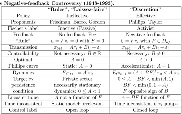
Using the above framework, table 1 summarizes distinctive features of the rules versus discretion (1948-1993) controversy.

Table 1: Rules versus Discretion, Stabilization Policy Ine¤ectiveness

ver-sus Negative-feedback Controversy (1948-1993).

“Rules”, “Laissez-faire” “Discretion”

Policy Ine¤ective E¤ective

Proponents Friedman, Barro, Gordon Phillips, Taylor

Fischer’s label Inactive (Passive) Activist

Feedback No feedback, Peg Negative feedback

“Rule” it = F t= 0 with F = 0 it= F t with F 2 Dnf

Transmission t+1= A t+ Bit+ "t t+1 = A t+ Bit+ "t

Controllability _{Not necessary: B 2 R Necessary: B 6= 0}

Optimal A = 0 A > 0

Phillips curve Static: A = 0 Accelerationist: A = 1

Dynamics Et t+1 = At 0 Et t+1 = (A + BF )t 0 < At 0 Target t persistence condition Private sector necessarily stationary dynamics: 0 A < 1 0 A + BF < min (A; 1) BF < min (0; 1 A) F opposite sign of B

Lucas critique A not a function of F A + BF function of F

Time inconsistent Static model: irrelevant Time inconsistent if t jumps

Prominent supporters of the “rules” side are Friedman (1948, 1960) and Barro and Gordon (1983a and b). Their implicit assumption is case 1 (A = 0) and static models without lags of the policy target (Blanchard and Fischer (1989), p.581). Barro and Gordon (1983a and b) consider a static Phillips curve (A = 0).

Prominent supporters of the “discretion” side are Phillips (1954b), Taylor (1993, 1999). They implicitly assume a dynamic model with trend (case 3: A > 1) and possibly with stationary persistence (case 2: 0 < A < 1). In case 2, persistence A is not too small so that the reduction of persistence subtracting BF < 0 is not negligible. Taylor (1999) and Fuhrer (2010) consider an accelerationist Phillips curve (A = 1), which may be related to trend in‡ation in the 1970s in the USA. Volcker’s discretionary monetary policy during 1979-1982 reversed non-stationary trend in‡ation into stationary in‡ation

0 A + BF < 1 A. The rule parameter F is a bifurcation parameter, for given values

of the parameters A and B of monetary policy transmission mechanism.

In control theory, the policy responses are always conditional on the transmission mechanism. It does not make sense to put forward a policy rule without specifying the policy transmission mechanism. For Nelson (2008, p.95), Friedman and Taylor agreed "on the speci…cation of shocks, policy makers’ objectives and trade-o¤s. Where they di¤ered was on the extent to which structural models should enter the monetary policy decision making process."

3

The Transplants of Control Tools from

Engineer-ing to Stabilization Policy

Smith did not refer to engines as an analogy when he explained the negative-feedback mechanism in the Wealth of Nations (see Mayr (1971)) even though he knew Watt and engineers’machines using negative-feedback. The concept of negative feedback was used by economist most of the time without a reference to engineer’s techniques until classic control emerged. With respect to the modeling of macroeconomic stabilization policy during the period of the rules versus discretion controversy 1948-1993, there have been three stages of implementation of control theory according to Zhou, Doyle and Glover (1996) and Hansen and Sargent (2008). The …rst one is classic control without a loss function in the 1950s, with proportional, integral and derivative (P.I.D) policy rules. The second one is optimal control including a quadratic loss function with a Kalman linear quadratic regulator, optimal state estimation with a Kalman …lter and stochastic optimal control merging both methods with the linear quadratic Gaussian model in the 1960s. The third stage is robust control which takes into account uncertainty on the parameters of the policy transmission mechanism in the 1980s.

3.1

The Fast Transplant of Classic Control

Tustin (1953), an electrical engineer at the University of Birmingham, mentions to have started in 1946 applying classic control methods used in electrical systems to Keynesian macro-models (Bissell (2010)). Phillips (1954a), an electrical engineer hired at the Lon-don School of Economics, wrote a two page book review on Tustin (1953) in the Economic Journal. He built the hydraulic computer MONIAC (Monetary National Income Ana-logue Computer) in 1949 (Leeson (2011)). The MONIAC is a series of connected glass tubes …lled with water where the ‡ow represented GNP and the feedback system

repre-sented the use of monetary and …scal policy. Phillips (1954b (from Phillips’PhD) and, 1957) used proportional, integral and derivative (P.I.D.) rules of classic control to stabilize an economic model using negative-feedback mechanism (Hayes (2011)). Taylor’s (1968) master thesis merged Phillips’(1961) model of cyclical growth with Phillips’(1954b) pro-portional, integral and derivative negative-feedback stabilization rules. Thirty-nine years after Phillips (1954b) and twenty-…ve years after Taylor’s (1968) P.I.D rules, the Taylor (1993) rule is a proportional (P) feedback rule of classic control. Taylor, in Leeson and Taylor (2012)), explains why he took sides with discretion:

I viewed policy rule as a natural way to evaluate policy in the kinds of macroeconomic models which I learned and worked on at Princeton and Stan-ford. It was more practical than philosophical or political. (Leeson and Taylor (2012))

We now highlight how classic control takes sides with “discretion”: The policy maker targets his preferred persistence of the time-series of policy targets, which determines his preferred speed of convergence of these policy targets to their long run equilibrium. For example, a central bank could do an in‡ation persistence targeting of an auto-correlation

of in‡ation of 0:8, satisfying a stability and negative feedback condition: 0 =

A + BF = 0:8 < min(A; 1). This decision is called in classic control “pole placement”,

because is a pole or a zero of the polynomial at the denominator of the Laplace transform

of the closed-loop system.

Accordingly, the policy maker decides on a policy rule parameter F = _BA = 0:8 A

B

in the case of a proportional feedback rule. For example, if there is a negative marginal e¤ect of the funds rate on in‡ation (B < 0), the policy rule F is an a¢ ne decreasing

function of the in‡ation persistence target .

Taylor’s (1999) transmission mechanism is an accelerationist Phillips curve (where xt

is the output gap and a is the slope of the Phillips curve) and an investment saving (IS) equation:

t+1= t+ axt, a > 0 and xt= b(it t), b > 0: (5)

So that the transmission mechanism of monetary policy is such as A = 1 + ab > 1:

t+1 = (1 B) t+ Bit with B = ab < 0: (6)

The Taylor principle states that the funds rate should respond by more than one to deviation of in‡ation from its long run target (F > 1). The Taylor principle corresponds to the classic control condition for negative-feedback rule parameters such that 0 <

A + BF < min(1; A), for models such that B < 0 and A = 1 B > 1(Taylor (1999)):

0 A + BF = 1 B + BF < 1 _{and B < 0 ) 1 < F <} B

A =

B

1 B: (7)

The upper bound condition on F corresponds to zero persistence of in‡ation.

3.2

The Fast Transplant of Optimal Control

The second step in the transfer of methods used in engineering to economic modeling is the introduction of optimal control in the 1950s, see Duarte (2009) and Klein (2015). In optimal control, a quadratic loss function is minimized subject to linear dynamic

equations. Using a certainty-equivalence property, normal disturbances with zero mean can be added to the model according to Simon (1956) and Theil (1957).

In the 1950s, Simon, Holt, Modigliani and Muth came to the Graduate School of Industrial Administration at the Carnegie Institute of Technology in Pittsburgh. Holt had come from an engineering background at M.I.T. and Simon’s father was an electrical

engineer after earning his engineering degree in Technische Hochschule Darmstadt.2

(Lee-son and Taylor (2012)). They applied control methods to microeconomics by computing variables for production, inventories and the labor force of a …rm. Optimal linear decision rules from linear quadratic models were computed for speci…c economic models of …rm’s production by Holt, Modigliani and Simon (1955) and Holt, Modigliani and Muth (1956), (Singhal and Singhal (2007)). Holt (1962) developed an optimal control model to analyze …scal and monetary policy.

Kalman (1930-2016), an electrical engineer, wrote the key paper for solving linear

quadratic optimal control (linear quadratic regulator, LQR).3 _{He extended the static}

Tinbergen (1952) principle, namely that there should be as many policy instrument as policy targets, to a dynamic setting. Kalman’s (1960a) controllability de…nition is such that a single instrument can control for example three policy targets, but in three di¤erent periods (Aoki (1975)). Masanao Aoki (1931-2018) was a Japanese professor of engineering at UCLA and California, Berkeley from 1960-1974, before switching …elds to economics. Kalman’s (1960a) linear quadratic regulator sets the solution of stabilization policy facing a quadratic loss function solving matrix Riccati equations. Textbooks include Sworder (1966) and Wonham (1974) among others.

The di¤usion of control techniques to macroeconomics was complementary to the development of large scale macroeconomic models:

Professor Bryson was o¤ering a course in the control theory in 1966 that caught the attention of a small group of economics graduate students and young faculty members at Harvard... Rod Dobell, Hayne Leland, Stephen Turnovsky, Chris Dougherty, Lance Taylor and I persisted... Two control engineers who had shifted their interest to economics – David Livesey at Cambridge University and Robert Pindyck at MIT – developed macroeco-nomic control theory models (in 1971 and 1972).... In May of 1972, a meeting of economists and control engineers was arranged at Princeton University by three economists (Edwin Kuh, Gregory Chow and M. Ishaq Nadiri) and a con-trol engineer. The meeting which was attended by about 40 economists and 20 engineers was to explore the possibility that the application of stochastic control techniques, which had been developed in engineering, would prove to be useful in economics as well (Athans and Chow, 1972).... Another British-trained control engineer, Anthony Healy, who was teaching at the University of Texas at the time, took an interest in economic models and applied the use of feedback rules to a well-known model that had been developed at the St. Louis Federal Reserve Bank (FRB). (Kendrick (2005), p. 7-8)

In the ongoing debate “discretion” versus “rules”, optimal control – with a policy maker minimizing a loss function – was used by macroeconomists in favor of

“discre-2_{Phillips’and Taylor’s fathers were also engineers, (Leeson and Taylor (2012)}

3_{He was invited to participate in the world econometric congress in 1980 in Aix en Provence, but his} paper was not published in Econometrica. He later received the highest honor of US science, the US medal of science in 2009.

tion”, whereas those in favor of “rules”model the private sector’s optimal behavior with stationary policy targets (0 < A = A0_+B0_F0 _{< 1). Nonetheless, even in this case, optimal}

control by the policy maker is still able to decrease the loss function further.

Optimal control is …lling a gap in the “pole placement” method of classic control

where the criterion for choosing the persistence of the policy target is not explicitly

stated (0 < = A + BF < 1). Kalman’s optimal control uses a quadratic loss function

with the possibility of discounting future periods with a factor and non-zero quadratic

cost of changing the policy instrument, R > 0, in order to ensure concavity. The relative cost of changing the policy instrument (R=Q) represents e.g. central banks’interest-rate smoothing or governments’ tax smoothing. In the case of the private sector, it corre-sponds to households’consumption smoothing or …rms’adjustment costs of investment. Maximize 1 2 +1 X t=0 t Q _t2+ Ri2_t , with R > 0, Q 0 and 0 < 1; (8)

subject to the same transmission mechanism as the one of classic control.

Solving this linear quadratic regulator yields two roots of a characteristic polynomial of order two, one of them stable, the other one unstable. For this reason, Blanchard and Kahn (1980) call this solution “saddlepath stable”, in a space which adds co-state variables (Lagrange multipliers) and state variables (policy targets). This implies that the dynamics of the state variables is stable, exactly like in classic control.

Optimal persistence is a continuous increasing function of the relative cost of

changing the policy instrument: _QR . The relation between the persistence of the

policy target and policy-rule parameter, A + BF = , is the same for optimal control

as for classic control. Unless the targeted persistence does not belong to the interval:

2i0; min A; 1_A h, a simple rule derived from classic control with an ad hoc targeted

persistence is observationally equivalent to an optimal rule R_Q , with identical

predictions and behavior of the policy maker. A reduced form of a simple rule parameter

F corresponds to an optimal rule F _QR with preferences R_Q. There exist preferences of

the policy maker that “rationalize” an estimated value of a simple rule parameter F to

be a reduced form of an optimal rule parameter F _QR .

Proposition 2 A rule pegging the policy instrument (i = 0, F = 0) is optimal for a

quadratic loss function (which is bounded if: A2

6= 1), with a …rst-order single policy maker’s instrument single-policy-target transmission mechanism:

(i) for stationary persistence of the policy target 0 < A < 1=p and for a zero weight (Q = 0) on the volatility of the policy target in the policy maker’s loss function.

(ii) for zero persistence of the policy target A = 0 and a positive weight Q 0 of the

volatility of the policy target in the loss function.

Proof. (i) With zero weight on the policy target (Q = 0), the relative cost of changing

the policy instrument is in…nite (R=Q ! +1), which corresponds to maximal inertia of the policy. Only the …rst of these two cases allows F = 0. In the second case, F = 0

0 F = A B A B , if 0 < A < 1 p , B < 0, 0 < 1: 1 A A B F = A B A B , if A > 1 p and B < 0, 0 < 1:

If the feedback parameter is zero (F = 0), optimal policy corresponds to a rule

(i = 0). The policy target dynamics t = A t 1 is not taken into account in the

expected loss function.

(ii) For A = 0 and for B 6= 0, the system is controllable with a non-zero e¤ect of the policy instrument on the policy target:

M in Q _t2+ Ri2_{t 1} subject to: t= Bit 1 ) Min Q + R

1 B2

2 t :

For each period with identical repeated optimizations, a rule (i = 0 = ) is the optimal

solution, whatever the magnitude of the relative cost of changing the policy instrument R=Q > 0.

The weakness of static analysis, however, was stated by Phillips (1954b) in a seminal paper on stabilization:

The time path of income, production and employment during the process of adjustment is not revealed. It is quite possible that certain types of policy may give rise to undesired ‡uctuations, or even cause a previously stable system to become unstable, although the …nal equilibrium position as shown by a static analysis appears to be quite satisfactory. (Phillips (1954a, p.290))

“Rules” are optimal for a static model A = 0, but in a dynamic model where A 1,

rules lead to instability and huge welfare losses. In addition, the hypothesis A = 0 cannot explain the observed persistence of all macroeconomic time series, which are stationary

if 0 < A < 1 or non-stationary if A 1. It cannot explain the variations of the

non-zero persistence of in‡ation (A + BF > 0), such as the acceleration of in‡ation or the disin‡ationary period during 1973 to 1982 with observed changes of the Fed’s policy behavior during Volcker’s mandate.

Optimal policy (rules) in a repeated static model of the transmission mechanism (A = 0, as with e.g. a Phillips curve) is never a modeling shortcut with results extended

by analogy to optimal policy in dynamic models of the transmission mechanism (A 1,

as with e.g. an accelerationist Phillips curve or a new-Keynesian Phillips curve) where discretion is optimal.

The above proposition for “rules” is bad news for the proponents of “rules” because “rules” are sub-optimal in dynamic models with policy makers using optimal control. Therefore, it was top of the research agenda of the proponents of “rules” in the contro-versy with discretion (that is, the opponents of Keynesian stabilization policy) to seek opportunities in order to add distortions in order to "prove" that optimal control tech-niques could not be used by policy makers for stabilization policy.

In addition, the above proposition renders useless Friedman (1953) results recently put forward by Forder and Monnery (2019) as a contribution for his Nobel prize. He

considers the simplest static model for the policy transmission mechanism:

CL= OL+ i:

The policy target randomly deviates from its zero equilibrium value with the value

OL if the policy instrument i is set to zero (open loop). After a change of the policy

instrument i, the closed loop value of the policy target is equal to CL. The policy maker’s

loss function is the volatility of the closed loop policy target 2

CL. The loss function is

obviously minimized 2

CL = 0 for this optimal negative feedback rule: i = OL, which

implies CL= 0, i OL = 1and i = OL. Friedman’s (1953) condition for sub-optimal

negative feedback rules is obtained after substitution of the transmission mechanism in the loss function:

2 CL = 2 OL + 2 i + 2 i OL i < 2 OL ) 1 i OL < 1 2 i OL :

Friedman (1953) discusses verbally the e¤ect of lags of the transmission mechanism. His mathematical formulation of the model, however, has no lags. As mentioned by Phillips (1954b), a negative feedback rule for a static model can drive instability in a dynamic model.

3.3

A Con‡ict between the Kalman Filter and Stochastic

Op-timal Control?

Additionally to the linear quadratic regulator (LQR, Kalman (1960a)) Kalman developed a …lter-estimate that recursively takes in each period the new data of the current period into account (Kalman (1960b)). This …lter is used, for example, in the global positioning system (GPS) since its inception in 1972.

It is …tting that at the conference [1st world IFAC conference, Moscow, 1960] Kalman presented a paper, ’On the general theory of control systems’ (Kalman, 1960) that clearly showed that a deep and exact duality existed be-tween the problems of multivariable feedback control and multivariable feed-back …ltering and hence ushered in a new treatment of the optimal control problem. (Bennett, 1996, p. 22).

Optimal trajectories derived from the linear quadratic regulator (LQR) and optimal state estimation using Kalman’s …lter for linear quadratic estimation (LQE) were uni…ed in the linear quadratic Gaussian (LQG) system. It is one of the main tools of Stochastic Optimal Control, see Stengel (1986) and Hansen and Sargent (2008). The Kalman …lter has been quickly implemented in rational expectations theory, even though an insu¢ cient emphasis on measurement can be observed.

The transplant of stochastic optimal control and the Kalman …lter to macroeconomics was very fast. For example, during his Ph.D. (1973) in Stanford, Taylor participated in seminars that discussed books linking control and time-series, such as Whittle’s (1963) Prediction and Regulation or Aoki’s (1967) Optimization of stochastic systems, see Leeson and Taylor (2012). Hansen and Sargent (2007) con…rm:

A pro…table decision rule for us has been, ‘if Peter Whittle wrote it, read it.’ Whittle’s 1963 book Prediction and Regulation by Linear Least Squares

Methods (reprinted and revised in 1983), taught early users of rational ex-pectations econometrics, including ourselves, the classical time series tech-niques that were perfect for putting the idea of rational expectations to work. (Hansen and Sargent (2008), p. xiii)

Independently of Kalman (1960b), Muth (1960) updated conditional expectations based on new information in a simple model. Hansen and Sargent (2007) highlight that Muth (1960) is a particular case of Kalman’s (1960b) …lter estimation. In the early 1970s, following Muth (1960), Lucas solved several rational expectations models using variants of a Kalman …lter (Boumans (2020)). Most of the time, Lucas used a Kalman …lter as a tool for solving theoretical models of rational expectations, instead of using it for what the Kalman …lter is designed for in the …eld of control, namely the practical empirical estimation of the state variables and of the parameters of the transmission mechanism using time series.

Based on the observations of a few Lucas’ papers in the early 1970s and following Sent (1998), Boumans (2020) infers that engineering mathematics did not unify optimal trajectories and optimal state estimation, whereas they were in fact uni…ed in the early 1960s in stochastic optimal control:

Engineering mathematics, however, is not one and uni…ed …eld. This pa-per shows that the mathematical instructions come from informational math-ematics, which should be distinguished from control engineering. (Boumans (2020)).

It may appear that the Kalman …lter and stochastic optimal control are distinct ap-proaches because Lucas used a Kalman …lter in theoretical papers in the early 1970s and later dismissed stochastic optimal control for policy makers in the Lucas (1976) critique. In basic engineering textbooks, such as Stengel (1986), however, optimal trajec-tories (Boumans’ (2020) “control engineering”) and optimal state estimation including the Kalman …lter (Boumans’(2020) “informational mathematics”) are merged into sto-chastic optimal control:

Not surprisingly, the control principle of chapter 3 and the estimation principles of chapter 4 can be used together to solve the stochastic optimal control problem. (Stengel (1986), p. 420)

This arti…cial split between policy makers’ optimal trajectories and optimal state estimation done by Lucas was in practice driven by the rules versus discretion controversy. This explains Lucas’ change of perspective and tools. Optimal control, and especially stochastic optimal control with a policy maker reestimating in each period the optimal policy is clearly a method favored by macroeconomists in the camp “discretion”. Hence, Lucas, as a proponent of “rules”, took the opportunity to break the dual approaches uni…ed by stochastic optimal control in two parts. The advocacy of particular theoretical views taking sides in a controversy and the selection of mathematical tools from control goes hand-in-hand. Scienti…c tools are part of the scienti…c rhetorics in order to convince a majority of scientists to opt for one side of the controversy.

The present study, then, provides a rationalization for rules with smooth monetary policy, exactly as did the earlier studies of Lucas, Sargent and

Wallace, and Barro. Similarly, it rationalizes the analogous …scal rule of continuous budget balancing and rules to stabilize the quantity of private money, such as larger reserve requirements for banks. (Lucas (1975), p. 1115) Barnett (2017) identi…es the di¤erent emphasis on measurement as the main method-ological di¤erence between rocket science and macroeconomics, with both …elds using control methods. William A. Barnett had a BS degree in mechanical engineering from MIT in 1963. He worked as an “rocket scientist” at Rocketdyne from 1963 to 1969, a contractor for the Apollo program. He then got a Ph.D. in statistics and economics from Carnegie Mellon University in 1974 at the same time as Finn Kydland. He worked for the models of the Fed soon after.

The di¤erent emphasis on measurement is very major, especially between macroeconomics and rocket science... In real rocket science, engineers are fully aware of the implications of systems theory, which emphasizes that small changes in data or parameters can cause major changes in system dynamics. The cause is crossing a bifurcation boundary in parameter space... But when policy simulations of macroeconometric models are run, they typically are run with the parameters set only at their point estimates. For example, when I was on the sta¤ of the Federal Reserve Board, I never saw such policy simulations delivered to the Governors or to the Open Market Committee with parameters set at any points in the parameter estimators’con…dence region, other than at the point estimate. This mind-set suggests to macroeconomists that small errors in data or in parameter estimates need not be major concerns, and hence emphasis on investment in measurement in macroeconomics is not at all comparable to investment in measurement in real rocket science. (Barnett (2017), p.22)

Lucas, Kydland and Prescott did not increase the emphasis on measurement with respect to modelers at the Fed in the 1970s. They had prior theoretical views taking sides for “rules” in the debate on rules versus discretion. As well as optimal control, using a Kalman …lter for optimal state estimation using macroeconomic time series would give a chance to challenge these prior views. Hence, it was a rhetorical strategy in the rules versus discretion controversy to challenge measurement and identi…cation strategies.

Lucas (1976) presented as impossible the econometric identi…cation of parameters in the case of reverse causality due to feedback rules. When confronting their model with data, Kydland and Prescott (1982) decided not to use Kalman-…lter optimal-state estimations and avoid identi…cation issues, but did simulations. The increased distance between econometricians and new-classical macroeconomists with respect to identi…cation issues in econometric estimations using a Kalman …lter, led to a selection bias with respect to the tools and the practice of control. In the …eld of control, the measurement of the transmission mechanism is viewed as much more important than theoretical models based on a priori hypothesis taking sides in a controversy. This increased the gap between the macroeconomics of stabilization policy and the …eld of control in the 1980s.

Kalman, who worked for the Apollo program, emphasized that the most important issue for stabilization of dynamic systems is the accuracy of the measurement and the estimation of parameters of the system of policy transmission mechanism (A and most importantly B and its sign) instead of a priori modeling of the real world. For Kalman, measurement is above all necessary for optimal policy rules, so one should not “separate”

…ltering estimation with data from optimal trajectories found with control. One should not separate macroeconomic theory from econometrics using macroeconomic time-series. By contrast, the linear quadratic gaussian (LQG) system merging optimal policy and Kalman …lter e¤ective estimation with macroeconomic time series has not been widely used during the the 1980s.

3.4

The Delayed Transplant of Robust Control

The third stage of control theory, namely robust control (Zhou et al. (1996), Hansen and Sargent (2008)), emerged in the following of Doyle’s (1978) two-pages paper presenting a counter-example where the Kalman linear quadratic Gaussian (LQG) model has not enough guaranteed margins to ensure stability.

Robust control assumes that the knowledge of the transmission parameters is uncer-tain on a known …nite interval with a given sign. In our example, it may correspond to Bmin < B < Bmax < 0. An evil agent tries to fool as much as possible the policy maker,

which reminds of Descartes (1641) evil demon:

I will suppose therefore that not God, who is supremely good and the source of truth, but rather some malicious demon, had employed his whole energies in deceiving me. (Descartes (1641))

The policy maker is the leader of a Stackelberg dynamic game against the evil agent. The policy maker is minimizing the maximum of the losses in the range of uncertainty on the parameters. Kalman’s solutions of matrix Riccati equation for the linear quadratic regulator remain instrumental for …nding the solutions of robust control.

For monetary policy, the uncertainty on parameters was put forward by Brainard (1967), so that, indeed, this is a very important issue. But the transplant of the new methods of robust control was delayed in the 1980s. Very soon after robust control tools emerged, Von Zur Muehlen (1982) wrote a working paper applying robust control to monetary policy which was never published in an academic journal. No major conference took place between leaders in the …eld of robust control and renowned macroeconomists like the ones described by Kendrick (1976) for stochastic optimal control in the early 1970s. Instead of at most three years for the spread of new tools from the …eld of control, one had to wait until the end of the 1990s, more than …fteen years. For now two decades, Hansen and Sargent (2008, 2011) transplanted robust control tools into macroeconomics (Hansen and Sargent (2008)), with still a limited number of followers in macroeconomics:

When we became aware of Whittle’s 1990 book, “Risk Sensitive Control” and later his 1996 book “Optimal Control: Basics and Beyond”, we eagerly worked our ways through them. These and other books on robust control

theory like Basar and Bernhard’s H1 _{“Optimal Control and Related Minimax}

Design Problems: A Dynamic Game” Approach provide tools for rigorously treating the ‘sloppy’ subject of how to make decisions when one does not fully trust a model and open the possibility of rigorously analyzing how wise agents should cope with fear of misspeci…cation.’ (Hansen and Sargent (2008), p. xiii)

The explanation of the delay for the transplant of robust optimal control is that the policy ine¤ectiveness arguments spread and took over for a while among in‡uential macroeconomists, according to Kendrick (2005):

However, it was a problem in the minds of many! As a result, work on control theory models in general and stochastic control models in particular went into rapid decline and remained that way for a substantial time. In my judgment, it was a terrible case of ‘throwing the baby out with the bath water’. The work on uncertainty (other than additive noise terms) in macroeconomic policy mostly stopped and then slowly was replaced with methods of solving models with rational expectations and with game theory approaches.... I believe that the jury is still out on the strength of these e¤ects and think that there was a substantial over-reaction by economists when these ideas …rst became popular. (Kendrick (2005), p.15)

We now re-evaluate the Lucas critique and the time-inconsistency theory that are at the origin of the long delay for using robust control methods and the relative scarcity of applied macroeconometric estimations using a Kalman …lter jointly with optimal policy with the linear quadratic Gaussian model.

4

The Impossibility to Identify the Parameters of the

Policy Transmission Mechanism

4.1

Lucas (1976) Critique

In popular terms, the Lucas critique states that (Keynesian) macroeconomic relations change with government policy. The Lucas critique is a parameter identi…cation problem in a system of dynamic equations including reverse causality due to a feedback control rule equation. The model of the last section of the paper of the Lucas critique (Lucas, 1976) can be stated in the form of the …rst-order single-input single-output model. We add our notations of the previous sections in brackets in the Lucas (1976) quotation. The

corresponding notations are: for the policy target: yt = t, for the policy instrument:

xt = it, and for the parameters of the transmission mechanism: = (A; B) which also

includes additive random disturbances "t. In order to avoid confusion with the control

notation F for the policy rule parameter, we change Lucas’notation of function F (:) into D(:):

I have argued in general and by example that there are compelling empir-ical and theoretempir-ical reasons for believing that a structure of the form

yt+1 = D (yt; xt; ; "t) [our notation: t+1 = A t+ Bit+ "t]

D (:)known, …xed, xt arbitrary will not be of use for forecasting and policy

evaluation in actual economies... One cannot meaningfully discuss optimal

decisions of agents under arbitrary sequences fxtg of future shocks. As an

al-ternative characterization, then, let policies and other disturbances be viewed as stochastically disturbed functions of the state of the system, or (paramet-rically)

xt= G (yt; ; t) [our notation: it= F t+ t]

where G is known, is a …xed parameter vector, and t a vector of

distur-bances. Then the remainder of the economy follows

where, as indicated, the behavioral parameters [or A + BF ] vary

system-atically with the parameters [or F ] governing policy and other “shocks”.

The econometric problem in this context is that of estimating the

function ( ) [or A + BF ]. In a model of this sort, a policy is viewed as a

change in the parameters [or F ] or in the function generating the values of

policy variables at particular times. A change in policy (in [or F ]) a¤ects

the behavior of the system in two ways: …rst by altering the time series

be-havior of xt; second by leading to modi…cation of the behavioral parameters

( )[or A + BF ] governing the rest of the system. (Lucas (1976, p.39-40))

The closed loop parameter (A + BF ) determines the persistence of policy targets. It depends on the policy rule parameter F as in all closed loop models including feedback mechanism in the …eld of control. The econometric problem is the identi…cation of para-meters A, B and F in a system of dynamic equations with reverse causality. In addition, in the scalar case, the true parameters B and F have opposite signs for the case of a negative-feedback mechanism (BF < 0).

Lucas (1976) over-stated that this parameter identi…cation problem cannot in princi-ple be addressed.

The point is rather that this possibility [of feedback rules] cannot in prin-ciple be substantiated empirically. (Lucas (1976, p.41))

Because the identi…cation of estimates of A and B cannot in principle be substantiated

empirically, then it is better to use rules such as it = 0and F = 0 instead of “discretion”

with a feedback rule parameter F 6= 0.

This reverse-causality parameter identi…cation problem is identical to the one of the private sector’s demand and supply price elasticities with respect to quantities, when there is negative feedback of supply on demand (section 2.1, Smith (1776) and Ezekiel’s (1938) cobweb model). The supply of goods should increase when price increases, whereas the demand of goods should decrease when price increases. But there is only one covariance for observed prices and quantities with a single sign.

According to Koopmans (1950), the identi…cation of B and F …nding opposite signs can in principle be substantiated empirically, if one …nds strong and exogenous instrumen-tal variables with distinct identi…cation restrictions for both the transmission mechanism (demand) and the feedback equation (supply). Finding these instrumental variables with their identi…cation restrictions is far from being easy with macroeconomic data. One an-swer is instrumental variables allowing identi…cation via identi…cation restrictions such as exogenous monetary policy shocks, exogenous in‡ation shocks or lags of some explanatory variables in vector autoregressive (VAR) models which include policy-target (in‡ation) and policy-instrument (funds rate) equations or lags of explanatory variables.

Although Lucas (1976) does not mention microeconomic foundations, it is often er-roneously claimed that microeconomic foundations are required because of the Lucas (1976) critique. From private sector’s demand and reverse causality of supply with neg-ative feedback, the private sector’s behavior estimates of elasticities are also subject to the Lucas (1976) critique. If the private sector’s behavior is modeled with microfounda-tions (section 3.2, intertemporal optimization using optimal control), the representative

household’s behavior includes an optimal policy-rule equation F0 _{besides the law of}

mo-tion of the private sector’s state variables with parameters (A0; B0) as in section 2.3. The Lucas critique applies as well: there is a system of two equations with reverse causality

and opposite signs for these two parameters: B0_F0 _{< 0. The private sector persistence}

parameter A0 _{+ B}0_F0 _{is not a structural parameter. Therefore, private sector’s}

micro-foundations are never an “answer” to the parameter identi…cation problem of the Lucas (1976) critique. Dynamic models of the private sector alone face also the Lucas critique, even without policy intervention where BF = 0 using section 2.3 notations.

Lucas’ rhetorical over-statement was successful, according to Blinder’s interview in July 1982 reported in Klamer (1984):

This is a case where people have latched upon a criticism. All you have to do in this country (more than in other places) right now is scream mind-lessly, “Lucas critique!”and the conversation ends. That is a terrible attitude. (Klamer (1984), p.166)

Instead of fostering a research agenda on identi…cation issues with reverse causality in applied econometrics, it convinced a number of macroeconomists that applied macro-econometrics was to be dismissed and hopeless. Macroeconomic theorists favored theory with the private sector’s microeconomic foundations using simulations, instead of tackling thorny identi…cation issues in econometrics.

4.2

Sims (1980) faces the Lucas critique: The VAR Price Puzzle

for Identifying

B and F with Opposite Signs

Several Keynesian applied econometricians, including Blinder, investigated the stability of reduced form estimates A + BF without …nding much change on several key equations from 1960 until 1979 or 1982 (Goutsmedt et al. (2019)). But it is possible to have unchanged reduced form persistence parameters, even when the “structural”parameters did change from period 1 (before 1973) to period 2 (after 1973): A1+ B1F1 = A2+ B2F2.

The di¢ cult step is to identify separately A, B and F for each period, knowing that there is a reverse causality with opposite signs (BF < 0) of the policy instrument and the policy target in the transmission mechanism (parameter B), on the one hand, and in the policy rule (parameter F ), on the other hand.

The Lucas critique was used as an explanation for the forecasting errors of large scale models such as the FMP model, for Federal Reserve-MIT-Penn. Another critique of large scale forecasting models was put forward by Sims (1980) with his vector auto-regressive models (VAR). Sims (1980) warned that some identi…cation restrictions (for example, constraining some parameters to be zero) were not tested in macroeconometrics in the 1970s.

But soon an unexpected anomaly of VAR models appeared, labeled the “price puzzle” (Rusnák et al. (2013)). We highlight that the VAR price puzzle is closely related to the Lucas (1976) critique. Impulse response functions obtain that in‡ation increases, following a shock increasing the funds rate. This is the opposite estimate of the expected

sign of the true model: bB > 0 > B. Indeed, impulse response functions are such that

the funds rate increases, following a shock increasing in‡ation, with the expected sign: b

F > 0. The identical sign for bB and bF comes from the fact that the sign of the covariance between the policy instrument and the policy target does not change with one or two lags. The price puzzle is such that bB > 0and bF > 0, so that there seems to be a positive feedback mechanism on in‡ation persistence of policy bA + bB bF > A, even during Volcker’s disin‡ationary policy with negative-feedback mechanism.

Estimating the correct sign of B is of utmost importance for policy advice. Negative feedback reduces the persistence of the policy target according to the condition: 0 < A + BF < A. This implies BF < 0. The sign of F should be the opposite of the sign of B. If one estimates wrongly that bB > 0 whereas its true value is B < 0, the policy advice will be F < 0, so that bBF < 0 < BF. Therefore, the policy advice will wrongly increase the persistence of the policy target:

0 < A + bBF < A < A + BF if wrong estimated sign B < 0 < bB: (9) Several econometric techniques have been used to reverse the sign of the “price puzzle” (Rusnák et al. (2013)). Perhaps some of them correctly managed to answer the Lucas (1976) critique for some data set. Walsh’s (2017) textbook restricts the description of the price puzzle measurement issue to half a page. Walsh’s (2017) textbook demonstrates that it has been easier to develop a large variety of theoretical micro-founded macroeconomic models con‡icting among themselves than to provide accurate measurements of A, B and F.

4.3

Kydland and Prescott (1982) face the Lucas’critique

For a representative agent of the private sector, Ramsey (1928) models a

negative-feedback mechanism for optimal savings or optimal consumption xt with consumption

smoothing (related to the notations R=Q for the linear quadratic approximation). This idea was formalized again independently by Cass, Koopmans and Malinvaud in 1965 (Spear and Young (2014)). Kydland and Prescott (1982) stuck to this idea adding auto-correlated productivity shocks zt.

Their model is a stock-‡ow reservoir model where the stock of wealth or the stock of

capital kt has an optimal set point k (De Rosnay (1979), Meadows (2008)). The stock

of capital is controlled by saving/investment in‡ows and it faces depreciation out‡ows. If the level of the stock is below its long run optimal target, consumption decreases proportionally according to a negative feedback proportional rule:

xt= F0kt+ F 0

zzt, kt+1 = (A0+ B0F0) kt+ (Akz0 + B0Fz0) zt with 0 < A = A0+ B0F0 < 1 ,

where both the consumption ‡ow and the capital stock are written in deviation from their long run target. Consumption also responds to an exogenous auto-correlated

pro-ductivity shock zt. To become rich, a poor representative households with capital below

its long run target (kt < 0) only needs to save more which implies his optimal

consump-tion is below its long run target (xt < 0). Hence, the poor representative household

replenishes his reservoir storing his stock of wealth to its optimal level (kt = 0).

When the relative cost of changing consumption (R=Q) increases, the policy rule pa-rameter decreases (consumption is less volatile) and the persistence of capital or wealth increases A or equivalently, the speed of convergence of capital towards equilibrium de-creases.

Kydland and Prescott (1982) send us back to Smith’s (1776) view that a negative-feedback mechanism always works within the private sector with supply and demand in-teraction. This time, the negative-feedback mechanism is related to the investment/saving market. It is a typical model including microeconomic foundations which faces the Lucas