Subjective Evaluation of Discomfort in Sitting Positions

(1)

HAL Id: halshs-00273179

https://halshs.archives-ouvertes.fr/halshs-00273179

Submitted on 14 Apr 2008

HAL is a multi-disciplinary open access

archive for the deposit and dissemination of sci-entific research documents, whether they are pub-lished or not. The documents may come from teaching and research institutions in France or

L’archive ouverte pluridisciplinaire HAL, est destinée au dépôt et à la diffusion de documents scientifiques de niveau recherche, publiés ou non, émanant des établissements d’enseignement et de recherche français ou étrangers, des laboratoires

Subjective Evaluation of Discomfort in Sitting Positions

Michel Grabisch, Jacques Duchene, Frédéric Lino, Patrice Perny

To cite this version:

Michel Grabisch, Jacques Duchene, Frédéric Lino, Patrice Perny. Subjective Evaluation of Discomfort in Sitting Positions. Fuzzy Optimization and Decision Making, Springer Verlag, 2002, 1 (3), pp.287-312. �10.1023/A:1019640913523�. �halshs-00273179�

(2)

Subjective evaluation of discomfort in sitting position

Michel Grabisch1∗, Jacques Duchˆene2_{, Fr´}_ed´_{eric Lino}3_{, Patrice Perny}1

1_{LIP6, Universit´}_{e de Paris VI, Paris, France}

2_{LM2S, Universit´}_{e de Technologie de Troyes, Troyes, France} 3_D´_{epartement Biom´}_{edical de l’Automobile, Nanterre, France}

Abstract

We study the modelling of the subjective sensation of discomfort for subjects seated during a long time, in terms of local discomforts. The methodology uses fuzzy measures and integrals in a multicriteria decision making perspective, which enables the modelling of complex interaction between variables. Results of the experiment are detailed, giving models with respect to different kinds of discomfort, and to different macro-zones of the body.

Keywords: subjective evalaution, multicriteria decision making, fuzzy measure, Choquet integral

1 Introduction

The evaluation of subjective sensations such as fatigue, stress, pain, etc., or subjective feelings and emotions, is a wide field of study, involving many different disciplines such as psychology, measurement theory, sensorial analysis, statistics and data analysis, etc. (see [7] for a survey of this topic). This makes the field particularly difficult, and much remains to be done to unify all the scattered contributions into a single perspective.

The introduction of the notion of fuzzy set by Zadeh [27], and later of the one of fuzzy measure by Sugeno [25], has been precisely motivated by an attempt to give a mathematical model of “subjectivity”. Fuzzy sets can be considered as a description of vagueness which cannot be captured by the classical notion of sets with precise boundaries (one of the examples given by Zadeh is: how to define the set of beautiful women?), hence is very suitable to model subjective sensations. On the other hand, Sugeno proposed fuzzy measures and fuzzy integral as a way to model the subjective feeling of uncertainty, by opposition to the objective flavour of probability measures, which can be based on statistical experiments. It is noteworthy to say that the first application of fuzzy measures and integrals, by Sugeno himself, was the (subjective) evaluation of woman faces, but in a way very different from Zadeh. Indeed, Zadeh had in mind graded membership to a set, while Sugeno constructed, using several attributes, a multidimensional model by the fuzzy integral. In fact, as remarked by Orlovsky and developed in his works [22], the two approaches concur, since the multidimensional model of Sugeno gives precisely the graded membership sought by Zadeh.

Later, many applications in subjective evaluation have been done using fuzzy measures and integrals (see [14] for a selection of them up to 1994, and [13] for more recent examples).

(3)

Our study is devoted to the modelling of the sensation of discomfort felt by a subject when seated during a long time, without the possibility to move. We will adopt the approach based on fuzzy measures and integrals, which we replace in the framework of multicriteria decision making to give it sound theoretical foundations.

The experiment tends to reproduce the situation where a car driver has to do a long distance drive, and so to remain seated without moving during a long time. The aim is first to analyze the sensation of discomfort felt by the driver (depending on the type of seat and the type of road), using a questionnaire where the subject can express his subjective feelings, and electromyographic sensors, and secondly, to analyze if the discomfort may cause some loss in ability to drive safely. The present paper restricts to the analysis of discomfort based on the questionnaire, since this part is particularly suited to the use of the above described approach.

2 Experimental setting

2.1 General outlay

The experimental apparatus is composed of a car seat placed on a vibratory bench, whose aim is to reproduce the vibrations generated by the road. The subject is seated and is watching a video on a screen in front of him, in order to keep attention fixed. To the right is fixed another screen with a joystick, which is used for performing some task.

The experiment consists in a sequence of 7 phases of about 20 minutes during which the subject is seated without moving, with or without vibration of the seat. After each phase, the subject is asked to fill in a questionnaire (see Section 2.2), and also to perform some reflex task and performance task, in order to measure the ability of the subject to concentrate on some tracking task.

There are 11 male subjects, 2 seats denoted hereafter A and B, and two modes, called static (no vibration), and dynamic (with vibration).

2.2 The questionnaire

The subject is asked to give an evaluation of his sensation of discomfort, describing its type, intensity and localization. More specifically:

• localization is coded according to the 38 zones defined on Fig. 1.

• types of discomfort are: vibratory, over-heating, pins and needles, hard point, contraction. • intensity is coded on a 0-10 scale, half-degrees are permitted. In order to help the subject to

assess numbers, some linguistic reference points are given as follows:

0=no discomfort, 2=perceptible, 4=sensitive, 8=painful, 10=unbearable.

The subject can indicate several zones, and possibly several types of discomfort (mixed discomfort) on the same zone. In this case, intensity is considered as a global one. For each zone, type(s) and intensity have to be given. Lastly, the subject gives an evaluation of the global sensation of discomfort he feels, on the same 0-10 scale.

(4)

Figure 1: Localization of discomfort

2.3 Aim of the experiment

The general aim of the experiment is to analyze the sensation of discomfort, and understand its causes and main factors, and secondly to evaluate to what extent discomfort can cause a loss in capability of attention and reflexes. Hence, apart from the questionnaire, tasks were performed by the subject, and electro-myographic signals were recorded at different places on the subject.

In this study, we restrict to the analysis of the questionnaire, that is, we intend to build a model of global discomfort based on local sensations of discomfort (see Fig. 2). Obviously, global discomfort cannot be explained solely by local discomforts, since other factors, less easy to grasp, intervene (e.g. boredom). It is however believed, and this study will confirm this view, that local discomforts mainly explain global discomfort. The obtained model could serve in a predictive purpose, but principally to explain which factors are important, and how they interact. Considering these local sensations as criteria, we use a multicriteria model which is explained in the next section.

3 Multicriteria evaluation model

3.1 General considerations

The model we intend to build has the form

d = f (d1, . . . , dk)

where d, d1, . . . , dk can be considered as satisfaction degrees of a given property, which can be

encoded between 0 (the property is not satisfied at all), and 1 (the property is fully satisfied). Property related to d is the global discomfort, encoded from 0 to 10, while those related to the di’s

(5)

Figure 2: Modelling global incomfort

Since the scale is the same for all variables, and assuming it is a difference or ratio scale, we can map it easily to [0, 1]. Note however the negative meaning conveyed by the property of discomfort: we may speak here of dissatisfaction.

Such models can be considered as a special type of multicriteria decision models (see e.g. [23] for a comprehensive survey of multicriteria decision methods), who computes a global score of a given alternative on the basis of its performance or score with respect to a set of criteria. The global score obtained can then be used as a way to rank alternatives.

This approach of aggregating scores for computing a global score is in the spirit of multiattribute utility theory [17], since scores on criteria are nothing else than utility values on attributes. The most classical way of aggregating utilites is the weighted sum, where weights express the relative importance of attributes. We use in this paper a much more general approach, based on Choquet integral. The following section introduces in a general way multicriteria decision models, and motivates the use of Choquet integral.

3.2 Multicriteria decision making by Choquet integral

Let us consider objects described by a set of descriptors or attributes X1, . . . , Xn, i.e. objects are

elements of the Cartesian product X1 × · · · × Xn. To each attribute Xi, we assign a criterion

Ci, that is, a mechanism which transforms values of the attributes (objective, physical, coming

from sensors) into preferences of the decision maker (DM for short). Most common forms of this mechanism are either based on pairwise comparisons of values leading to several binary relations (outranking approaches, see [23]), or more simply, the mechanism is a set of functions ui: Xi −→ R,

i = 1, . . . , n, assigning a satisfaction degree to each value of the attribute Xi. The functions ui are

called “utility functions” (this view is known as multiattribute utility theory [17]). More restrictively, when functions are valued on [0, 1], they can be viewed as membership functions of the fuzzy sets of satisfying or acceptable objects, relatively to a given attribute.

From now on, we adopt the second point of view (multiattribute utility theory), and consider functions valued on [0, 1], as explained in Section 3.1. For any object x ∈ X, whose values of the attributes are x1, . . . , xn, the satisfaction degrees (or scores for short) are u1(x1), . . . , un(xn)

according to the above notations. Since we deal only with scores from now on, we denote them as a1, . . . , an, or more shortly a∈ [0, 1]n. For commodity, we denote by N = {1, . . . , n} the (index)

(6)

set of criteria.

The aim of the multiattribute utility approach is to assign to each vector of scores a a global score, denoted u(a), which takes into account the different criteria describing the preferences of the decision maker on each attribute, in a way which reflects the attitude of the decision maker when considering simultaneously several criteria. Note that u is a function from [0, 1]n to some real interval (yet to be precised, but [0, 1] seems to make sense), and thus can be considered as an aggregation operator, a topic which has been widely studied in the fuzzy logic community (see e.g. [2, 26, 15])

More specifically, we make the assumption that the mechanism of decision of the DM can be described by two components:

• the intra-criterion preference, which describes to what degree values of a given attribute Xi are satisfying for the DM. This is captured by the utility function ui. Methods such as

MACBETH [3, 4] are able to derive such utility functions, making the assumption that the satisfaction degrees lie on a difference scale, i.e. a numerical scale where difference of numbers are meaningful. Moreover, MACBETH ensures that all utility functions are commensurable, i,e, they map on the same scale, and values taken by ui and uj, i6= j, can be meaningfully

compared.

• the inter-criteria preference, which describes to what degree coalitions of criteria (i.e. any subset of N ) are important for the decision.

Let us assume the first part being achieved, and detail the second part. We ask the decision maker to tell his/her preference over objects whose vectors of scores are of the form (1A, 0Ac), for every A⊂

N , which means, criteria belonging to coalition A are fully satisfied (score=1), while other criteria are not satisfied at all (score=0). Let us call binary objects such objects. By suitable methods, such as the MACBETH methodology, it is possible to derive through questioning a numerical representation of this preference on a difference scale (see [12, 11] for a detailed construction). Let us call µ : P(N) −→ R this numerical representation, where P(N) is the set of all subsets (coalitions) of N . For any A ⊂ N, the quantity µ(A) reflects for the decision maker the level of satisfaction of the object whose vector of score is (1A, 0Ac). Concerning µ, it seems reasonable to

make the following assumptions:

(i) Since the object (1N, 0∅) is clearly the best possible and (1∅, 0N) the worst possible, the values

of µ(N ) and µ(∅) are the bounds of the image of µ. It seems reasonable to take µ(∅) = 0 and µ(N ) = 1. Indeed, µ(∅) is the satisfaction of an object having (0, 0, . . . , 0) as vector of scores, so its global score should be 0 (and similarly for µ(N )). Hence, µ takes its values in [0, 1]. (ii) Let us consider some binary act (1A, 0Ac), A ( N . If we add a criterion i∈ N \ A to A, thus

building the binary object (1_A∪i, 0(A∪i)c), this new object is at least as good as the original one

(1A, 0Ac), since criterion i, which was not satisfied before, is now fully satisfied, the remaining

criteria being fixed. Thus, it is reasonable to assume what we call monotonicity, i.e. A_{⊂ B ⇒ µ(A) ≤ µ(B).}

A set function µ :P(N) −→ [0, 1] satisfying the two above requirements (i) and (ii) is called a fuzzy measure [25] or a capacity [1]. In the related litterature, µ(A) is often interpreted as the importance of coalition A to make decision, although the true meaning is what we explained above.

Recalling that the meaning of µ(A) is the satisfaction degree of object (1A, 0Ac), we see that

(7)

hypercube [0, 1]n, so that µ and u coincide on these vertices. Since u must be defined for every point in [0, 1]n_{, we can say that u is an extension of µ on [0, 1]}n_{. It means that importances of}

coalitions and the aggregation operator are closely linked: one cannot choose them independently. This fact is most of the time overlooked in applications.

Since the definition of µ involves 2n values, which may cause some interpretation problem in terms of importance of criteria, a convenient concept is the one of Shapley index [24], coming from cooperative game theory. For any criterion i∈ N, the Shapley index of i is defined by:

φi:=

X

K⊂N\i

(n− |K| − 1)!|K|!

n! [µ(K∪ {i}) − µ(K)]. (1)

Roughly speaking, the Shapley index φicomputes the average contribution of criterion i in all

coali-tions, the average being weighted by a coefficient taking into account the cardinality of the coalition. In this sense, it can be taken as definition of the average importance or average contribution of a single criterion for the decision process. The Shapley index satisfies Pn

i=1φi = µ(N ) = 1, so that

the sum of importance degrees is a constant. The idea to use the Shapley index for multicriteria decision making is due to Murofushi [20].

So far, we have shown that the aggregation function u is to be an extension of µ. Of course, infinitely many extensions exist. Grabisch et al. have shown that, under a small set of assumptions on the preferences of the decision maker, the Choquet integral (see below) is a candidate among others [12, 11]. Being a little more restrictive on the assumptions and restricting to positive scores1, Labreuche and Grabisch have shown the only solution is the Choquet integral [18].

Definition 1 Let f : N −→ R+_{, and µ be a fuzzy measure. Let us denote f (i) by f}

i,∀i ∈ N. The

Choquet integral of f w.r.t. µ is defined by: Cµ(f ) :=

n

X

i=1

(f(i)− f(i−1))µ({(i), . . . , (n)})

where (·) means a permutation of the elements of N such that f(1)≤ · · · ≤ f(n), and f(0):= 0.

The Choquet integral is different from what is called the fuzzy integral proposed by Sugeno [25] (or Sugeno integral). The Sugeno integral can be useful in situations where it is not possible to build difference scales for the ui’s and µ (see [10] for a study in this situation). For general properties of

the Choquet integral in a finite setting, see [14, 5]. An important property of the Choquet integral is monotonicity, that is, for all i∈ N:

Cµ(a1, . . . , ai, . . . , an)≥ Cµ(a1, . . . , a0i, . . . , an) whenever ai≥ a0i. (2)

If the fuzzy measure is additive, i.e. µ(A_{∪ B) = µ(A) + µ(B) whenever A and B are disjoint,} then in our finite setting, µ(A) =P

i∈Aµ({i}) for any A ⊂ N. Denoting for simplicity µ({i}) by

µi, it is easy to see that, for additive fuzzy measures, the Choquet integral reduces to:

Cµ(f ) = n

X

i=1

µifi.

We recognize here the classical weighted sum, the most widely used operator in multicriteria decision making and multiattribute utility theory. The above development shows well how this classical

1

(8)

model can be embedded into our general construction. It shows also how restrictive is this model, since it means that for every binary object (1A, 0Ac), its global score is merely the sum of the global

scores of (1_{i}, 0_{i}c), i∈ A. By using fuzzy measures, we can be far more general, and model what

is often called interaction between criteria. This means the following: taking the particular case of N ={1, 2} and considering µ({1}) = µ({2}), three extremal situations can occur [16, 12]:

1. The decision maker considers that objects having as vectors of scores (1, 0), (0, 1) and (1, 1) are equally good. In other words, it is enough to satisfy one the criteria, and the satisfaction of both does not add any satisfaction more. This means that µ({1}) = µ({2}) = µ(N) = 1. We say that criteria 1 and 2 are substitutive or redundant, and have a negative synergy or interaction. It easy to check that in this case, the Choquet integral reduces to

Cµ(f ) = f1∨ f2

where∨ denotes maximum, i.e. scores are aggregated disjunctively.

2. The decision maker considers that objects having as vectors of scores (1, 0), (0, 1) are not more satisfactory than the worst object (0, 0). In other words, both criteria have to be satisfied, otherwise the object is not satisfactory. This means that µ({1}) = µ({2}) = µ(∅) = 0. We say that criteria 1 and 2 are complementary, and have a positive synergy or interaction. In this case, the Choquet integral becomes:

Cµ(f ) = f1∧ f2

where∧ denotes minimum, i.e. scores are aggregated conjunctively.

3. The decision maker considers that objects having as vectors of scores (1, 0), (0, 1) are mid-way between the worst and better objects. This means that µ({1}) = µ({2}) = 12, which

entails additivity of the fuzzy measure. We say that the criteria are independent, or have no interaction. As noted before, the Choquet integral reduces to:

Cµ(f ) =

1

2(f1+ f2).

The term “independent” comes from the fact that scores on criteria add independently. The Choquet integral makes a mixture of these extreme attitudes. More precisely, as shown in [9], in the case of 2 criteria, the Choquet integral is the convex sum of min, max and the 2 dictators (or projections), i.e. the aggregation function which assigns as global score one of the scores.

Generalizing the above reasoning to any number of criteria leads to the definition of an inter-action index for 2 criteria, as proposed originally by Murofushi and Soneda [21].

Iij :=

X

K⊂N\{i,j}

(n− |K| − 2)!|K|!

(n− 1)! [µ(K∪ {i, j}) − µ(K ∪ {i}) − µ(K ∪ {j}) + µ(K)]. (3) By definition, criteria having a positive (resp. negative) interaction are such that Iij > 0 (resp.

Iij < 0), and independent criteria are such that Iij = 0. Note that Iij = 0, for all i, j if µ is additive.

Later, Grabisch has generalized this notion to any number of criteria, leading to the following definition of the interaction index [8], defined for all coalitions (including the empty one), which is:

I(A) := X K⊂N\A (n_{− |K| − |A|)!|K|!} (n− |A| + 1)! X B⊂A (−1)|A|−|B|µ(K∪ B), ∀A ⊂ N. (4)

(9)

Note that I({i}) = φi, and I({i, j}) = Iij. Also, it is easy to show that for an additive measure,

I(A) = 0 whenever |A| > 1, and φi = µ({i}). It is interesting to note that giving I(A) for all

A⊂ N permits to recover the fuzzy measure µ: I is merely another representation of µ (see [8] for details).

The above exposition has shown the richness of such kind of model, which can range from pure conjunctive to pure disjunctive aggregation. Moreover, one can have (almost) arbitrarily conjunctive aggregation between i and j, and disjunctive aggregation between k and l. This richness has however to be paid by a high complexity of the method. Indeed, the definition of the fuzzy measure involves 2n values, which may be not easy to obtain from the decision maker. Also, their interpretation may be not easy, or only partial, since the Shapley index and the interaction index for pair of criteria give a clear, but only partial, description of the fuzzy measure. To overcome this serious limitation, Grabisch has proposed the concept of k-additive measure, defined as follows. Definition 2 A fuzzy measure is said to be a k-additive measure if I(A) = 0 for all coalitions of more than k elements, and there exists at least one A of exactly k elements such that I(A)_{6= 0.} A 1-additive measure is an ordinary (additive) measure in the classical sense. A 2-additive measure is entirely described by the Shapley index and the interaction index for pair of criteria, needing only

n(n+1)

2 − 1 values to be defined, and so is a good compromise between richness and complexity. It

is worth noting that the Choquet integral has a particularly interesting form when µ is 2-additive: Cµ(a) = X Iij>0 (ai∧ aj)Iij+ X Iij<0 (ai∨ aj)|Iij| + n X i=1 ai(φi− 1 2 X j6=i |Iij|), ∀a ∈ [0, 1]n, (5)

with the property that φi− 1₂P_j6=i|Iij| ≥ 0 for all i. This formula shows clearly the disjunctive

and conjunctive effects of negative and positive interaction between criteria. Note also that the Shapley index lies in the linear part, and that the above formula is in fact a convex sum.

3.3 Identification of the fuzzy measure in subjective evaluation problems

The above section introduced the Choquet integral as a general way of aggregating criteria, and our presentation was done in the spirit of multicriteria decision making. The evaluation problem however, has a different perspective, since the available data is not exactly of the same nature. In the above presentation, the fuzzy measure was deduced from preferences of the decision maker on binary objects, which are clearly hypothetical objects in a real situation. In subjective evaluation, the subject expresses his/her feeling on real objects or situations, which cannot be chosen or constructed arbitrarily, so the above construction of µ becomes impossible.

To overcome this problem, we use a least square estimation of µ, which makes necessary to have the following data for each object: a global score of the object, and scores for each criteria, all scores being given on the same difference scale, and being commensurable (see Section 3.2). Specifically, let us denote for each object xl ∈ X1× · · · × Xn, l = 1, . . . , N , its global score by el,

and the vector of scores on criteria by al_{, with e}l _{∈ [0, 1] and a}l _{∈ [0, 1]}n_{. The aim is to find µ}

which minimizes the squared error E2:

E2 := N X l=1 h Cµ(al)− el i2 .

It is shown in [14] that this problem can be put into a quadratic optimization problem under linear constraints:

(10)

Number of variables 2 3 4 5 6 7 8 9 10

1-additive 1 2 3 4 5 6 7 8 9

2-additive 1 5 9 14 20 27 35 44 54

3-additive ∗ 6 13 24 40 62 91 128 174

General 2 6 14 30 62 126 254 510 1022

Table 1: Number of parameters of the models

minimize 1₂utDu + ctu

under the constraint Au + b≥ 0

where u is a (2n _{− 2) dimensional vector containing all the coefficients of the fuzzy measure µ}

(except µ(∅) and µ(N) which are fixed), D is a (2n_{− 2) dimensional square matrix, c a (2}n_{− 2)}

dimensional vector, A a n(2n−1− 1) × (2n_{− 2) matrix, and b a n(2}n−1_{− 1) dimensional vector.}

Standard methods of quadratic programming can be used to solve this program. Solution is not unique in general (see [19]). The optimization can be performed also under the constraint of getting a k-additive measure, for a given k.

Since the above method could not work very well when n is large and/or too few data are avail-able, Grabisch has proposed a sub-optimal method called Heuristic Least Mean Squares (HLMS) [6] to solve the above problem. HLMS can accept very few learning data, since it is based on the idea of attraction to a central point (which is the equidistributed fuzzy measure µ(A) := _|A|1 ): any input datum moves away the current point according to the magnitude of error, in the direction given by the gradient. The fewer data, the less movement is done from the equidistributed measure. However, the algorithm does not work for k-additive measures.

3.4 Construction of the model

We begin by a detailed analysis of the problem. For each datum, we have the following information, which constitutes the list of potential variables of the model:

• the subject number (∈ {1, . . . , 11}) • the seat (A or B)

• the mode (dynamic or static)

• the number of the task (∈ {1, . . . , 7})

• the list of zones where an discomfort has been felt (maximum 38 zones)

• for each zone, a list of felt discomforts (any subset of the 5 types of discomfort).

Based on the above considerations, the total number of potential variables is 11×2×2×7×38×25_,

which amounts to 1220 variables! On the other hand, the number of available data is 86, after elimination of data unsuitable for analysis.

Usually a multicriteria model should not exceed a dizain of criteria on a single level. We indicate in Tab. 1 the number of parameters requested by the different types of models, according to the number of variables (criteria), up to 10. After this, it seems that a reasonable limit should be 5 variables, unless a linear (1-additive) model is used.

(11)

It is then necessary to reduce drastically the number of variables by suitable projections and choice of significant variables. The first 4 potential variables (subject, seat, mode, task) are con-sidered as contextual variables rather than explicative variables, since they describe the situation of the experiment. On the other hand, all variables concerned with local discomfort can be ex-plicative variables for global discomfort. Thus, a model can be built for each combination of values of contextual variables. This being clearly too much detailed, we examine which combinations are relevant or feasible for the analysis.

• analysis by subject vs. global analysis of all subjects. It is possible to build a model per subject, or to consider all the subjects together. This last way to proceed will smooth small individual differences, at the risk of giving an average model not reflecting any reality if subjects with very different reactions coexist. On the contrary, the first way will clearly bring into light these differences. However, the number of data per subject is too low for considering this analysis as meaningful.

• analysis by seat vs. global analysis of the 2 seats. It could be interesting to build a model per seat, since they are known to be very different (seat A is a very comfortable seat for high class vehicles, and seat B is intended for small vehicles, and is rather hard). Doing this, the model could be used to explain causes of discomfort for each seat. The number of available data is 41 for seat A, and 45 for seat B.

• analysis by mode vs. global analysis of the 2 modes. Here also it should be interesting to create one model per mode, since the sensations felt by the subject are very different. The number of available data is 62 for the dynamic mode, and 24 for the static mode.

• analysis by task vs. global analysis of the 7 tasks. A global analysis would erase the time aspect of the experiment. More specifically, one could think of making a 1-order recursive model of the type y(t) = f (y(t− 1), x1, . . . , xk). However, here again the small number of

data forbids this kind of analysis.

Due to the low number of data, more detailed combinations are not possible.

It remains to examine how to reduce to 5 criteria the high number of explicative variables created by the different zones and types of discomfort. We propose two different approaches.

• perform a summation of discomfort sensations of a given type on all zones of the body. Since there are 5 different types of discomfort, this makes precisely 5 variables.

• in a orthogonal way, perform a summation of discomfort sensations of different types in a given zone. Since the total number of zones is too large (38), and such a fine cut-out is unnecessary, we have clustered the zones into 5 “macro-zones”, which are: arms, legs, lower back, upper back and chest. These macro-zones are indicated on Fig. 3.

A problem however subsists since in both cases, we perform a “summation” on sensations of dis-comfort, but what is the precise meaning of summation here? We make the assumption that for the human sensory system, sensations add logarithmically. This is known to be true for hearing and sight, and it seems reasonable to consider it true also for precise types of discomfort (that is, vibratory, over-heating, pins and needles, hard point and contraction). The method is illustrated on Fig. 4. Let us consider the discomfort scale [0, 10]. A stimulus of intensity x is perceived as a discomfort proportional to log_K(x), with an appropriate constant K. Assuming K = 1, a stimulus of double intensity 2x turns into an increasing of log_K2 for the discomfort. Note that value 0 on

(12)

Figure 3: Definition of the macro-zones

Figure 4: Logarithmic sum of discomfort

the scale corresponds to the sensitivity threshold, under which no sensation is perceived. Then, considering sensations y1, . . . , yk to be summed, the global sensation y is:

y = log_K " _k X i=1 Kyi #

The same method can be applied for zones where several types of discomfort are felt. We make the assumption that these discomforts are perceived with equal intensity on the zone (principle of the insufficient reason). Thus, if k is the number of discomforts perceived on the zone, and if y is the perceived level of discomfort on this zone, the level yi corresponding to discomfort i is given by:

yi = y− logK0k,∀i = 1, . . . , k.

It remains to determine the constants K and K0. We do this in an intuitive way, considering the meaning of the linguistic labels attached to the scale [0, 10]:

(13)

0=no discomfort, 2=perceptible, 4=sensitive, 8=painful, 10=unbearable.

Concerning K, the natural logarithm seems to fit well (K = e): supposing 10 zones with an intensity y, the sum gives y + ln 10 = y + 2.3. Taking various values of y leads to a plausible result.

On the other hand, we have chosen K0= 2. It means that for a zone with 2 types of discomfort with a global level y, the level for each type of discomfort is y− ln 2 = y − 0.69.

Examining the data obtained with these constants seems to indicate that they are correct. For each identification of models, the following methods have been used (see Section 3.3): • optimization by HLMS, with α = β = 0.01, number of iterations = 300

• quadratic optimization (full general Choquet integral model) • k-additive model, with k = 1, 2, 3.

4 Experimental results

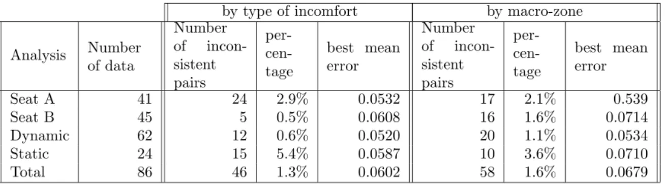
We present a summary of the results obtained, that is considering all data2together (called hereafter “Total”), all data for the dynamic mode, the static mode, seat A and seat B. We have discarded the results concerning the subjects individually, since they are not so significative. Table 2 shows the number of pairs of inconsistent data, and the percentage of them among all pairs of data. A pair of data ((al; el), (ak; ek)) is said to be inconsistent if

el> ek and al_i≤ aki,∀i ∈ N,

where el ∈ [0, 1] is the global score, and al _{∈ [0, 1]}n _{the vector of scores. This gives a precise idea}

of the validity of the multicriteria approach (whatever it is, since monotonicity is a fundamental requirement of any multicriteria method. Of course, the Choquet integral satisfies monotonicity, see (2)). The table gives also the best mean absolute error performances. An excellent adequation of

by type of incomfort by macro-zone

Analysis Number of data Number of incon-sistent pairs per- cen-tage best mean error Number of incon-sistent pairs per- cen-tage best mean error Seat A 41 24 2.9% 0.0532 17 2.1% 0.539 Seat B 45 5 0.5% 0.0608 16 1.6% 0.0714 Dynamic 62 12 0.6% 0.0520 20 1.1% 0.0534 Static 24 15 5.4% 0.0587 10 3.6% 0.0710 Total 86 46 1.3% 0.0602 58 1.6% 0.0679

Table 2: Validity of the multicriteria approach

data with the multicriteria approach (low percentage of inconsistent pairs), as well as an excellent modelling ability of Choquet integral (average absolute error is most often lower than 0.05, which represents an error of 5%) can be observed from the table. By contrast, the linear model (1-additive) leads to errors which are the double or quadruple. This model will not be commented hereafter.

2

A datum is a pair (a; e), where a∈ [0, 1]n

(14)

In appendix, we give the numerical results obtained for the “Total” analysis only, giving various modelling errors, the Shapley value and the interaction index matrix for pairs of criteria, and if any, veto and favor effects.

We comment now the results for all analyses.

• Total, by type of discomfort: the criteria the most important are over-heating and contraction, with a slight preference for the first one. Then comes criterion hard point. Criterion vibratory is negligible. The model is globally of the ”max” type, i.e. the criteria act as favors3. In particular, pairs (over-heating and contraction) are the most redundant. There is a very good agreement of the different models for these results.

• Total, by macro-zone: the 2 criteria which clearly prevail are upper back and arms. In particular, legs seems to be negligible. Only model HLMS gives a slightly different conclusion, where lower back is as important as upper back. Concerning interactions, one can see a very strong redundancy between upper back and arms, the other pairs being almost independent (except (legs, lower back) and (arms, lower back)).

• Seat A, by type of discomfort: all models are in accordance to conclude that criterion over-heating is the most important, followed immediately by criteria contraction and hard point. Criterion pins and needles is particularly negligible. Pairs (over-heating, contraction) and (over-heating, hard point) are particularly redundant, the other being almost independent.

• Seat A, by macro-zone: there is a slight discrepancy between optimal methods, which place criteria upper back and arms clearly above the others, those being almost negligible, and HLMS which concludes that lower back dominates, followed by arms and upper back. Pair (arms, upper back) is strongly redundant in all models, then often (legs, upper back) and (legs, arms). The other criteria are almost independent.

• Seat B, by type of discomfort: criteria contraction, hard point and over-heating are the most important, more or less equal. Criterion vibratory is completely negligible. The model is globally of “max” type, with some important effects of favor for contraction, hard point and over-heating. The most redundant pair is (over-heating, hard point). • Seat B, by macro-zone: upper back and lower back markedly dominate the other

cri-teria, then comes criterion legs. There is a conflict for criterion arms, which is considered totally useless by the optimal methods (k-add, quadratic), and rather important by HLMS. The model is strongly of the ”max” type, all the criteria (except arms) being favors. The most redundant pairs are (lower back, ) and (lower back, legs).

• static, by type of discomfort: on the whole, the models are in accordance to conclude that criterion over-heating is strongly dominating, followed by criterion contraction. Criterion hard point is clearly below with respect to other analyses. Criterion vibratory is totally negligible. Pair (over-heating, contraction) is strongly redundant, the other pairs are almost independent. However, there is a slight tendency for pair (hard point, contraction) to be complementary.

3

However, due to the negative meaning of the discomfort, it means instead a veto effect: it suffices that only one type of discomfort appears to cause a global discomfort.

(15)

• static, by macro-zone: for all the models except the quadratic one, criteria lower back and upper back are equally important and clearly preponderant. By contrast, for the quadratic model, preponderant ones are criteria lower back and arms. Criteria legs and chest are almost negligible on the whole. Important criteria are always strongly redundant between them, while other combinations exhibit independency.

• dynamic, by type of discomfort: here criteria over-heating, contraction and hard point are again the important ones, while it is not clear which is the most important one. Criterion vibratory is the less important. The model is globally of the “max” type, and most redundant pairs can be found among criteria over-heating, contraction and hard point.

• dynamic, by macro-zone: criteria upper back and arms are clearly preponderant. Curi-ously, lower back is considered as completely negligible by the optimal methods, while it is an important criterion for HLMS. Pair (arms, upper back) is clearly redundant.

Based on the above comments, we can draw the following conclusions for the multicriteria modelling: • up to very few exceptions, the different models give conclusions which agree on the whole. Even if discrepancies exist, they remain on criteria of secondary importance. Models differ essentially when they are few data, so that their validity becomes questionable. There are more discrepancies in the analysis based on macro-zones than on types of discomfort. • the “Total” analysis, as well as most of the other analyses, reveals the three most

impor-tant criteria for discomfort, which are over-heating and contraction, and then criterion hard point, a little less important. Criterion vibratory does not seem to influence global discomfort.

The model aggregates criteria in a disjunctive form (“max” type), i.e. all criteria are favors to some degree. In other words:

It suffices that one discomfort of the type over-heating, contraction or hard point appears for a global discomfort to be felt. No sensation of discomfort can alleviate another sensation of discomfort.

• the analysis by macro-zone shows that macro-zones upper back and arms, and lower back to a lesser extent, are the most explicative ones. Macro-zone legs seems to be without influence. The model of global discomfort can be epxressed by a disjunction between upper back and arms while other pairs of criteria are almost independent. In other words:

It suffices that a discomfort is felt in arms or the upper back for a global discomfort to be felt. Discomfort sensations appearing in other macro-zones (especially lower back) will reinforce the global sensation of discomfort.

• the analysis by seat shows slight differences between them. For seat A, over-heating is the first cause of discomfort, while for seat B, over-heating is as much important as the presence of hard points. We could have expected more disparities.

• the analysis by mode also shows some differences. Criterion over-heating predominates for the static mode, and hard point is clearly below, while for the dynamic mode, these 3 criteria are equally important.

(16)

Before ending the paper, we give the explicit form of the models for the “Total” analysis, in the case of a 2-additive measure, using formula (5).

1. Analysis by type of discomfort. Variables a1, . . . , a5 are discomfort levels of vibratory,

over-heating, pins and needles, hard point and contraction respectively. e is the global discomfort level, with a precision of 10−3.

e =0.022(a2∧ a3) + 0.337(a2∨ a4) + 0.256(a2∨ a5) + 0.163(a3∨ a5) + 0.142(a4∨ a5)

+ 0.003(a1∨ a3) + 0.028a3.

2. Analysis by macro-zone. Variables a1, . . . , a5 are discomfort levels at legs, arms, lower

back, upper back and chest respectively. e is the global discomfort level, with a precision of 10−3.

e =0.517(a2∨ a4) + 0.134(a4∨ a5) + 0.122(a2∨ a3) + 0.095(a1∨ a3) + 0.051(a3∨ a4)

+ 0.039(a1∨ a5) + 0.043a5.

We can see that in both cases, the linear part of the model is almost zero.

5 Conclusion

The work has shown the descriptive power and accuracy of the methodology based on fuzzy mea-sures and the Choquet integral. Compared to a linear model. i.e. a standard regression analysis, the proposed methodology, which can be considered as a non linear regression analysis, is more flexible, and brings information on interaction among variables. Also, the obtained model is easy to interpret due to the clear meaning of the notion of interaction.

6 Acknowledgment

This work has been partially supported by French DGA, Contract 95/169.

References

[1] G. Choquet. Theory of capacities. Annales de l’Institut Fourier, 5:131–295, 1953.

[2] D. Dubois and H. Prade. A review of fuzzy set aggregation connectives. Information Sciences, 36:85–121, 1985.

[3] C.A. Bana e Costa and J.C. Vansnick. A theoretical framework for Measuring Attractiveness by a Categorical Based Evaluation TecHnique (MACBETH). In Proc. XIth Int. Conf. on MultiCriteria Decision Making, pages 15–24, Coimbra, Portugal, August 1994.

[4] C.A. Bana e Costa and J.C. Vansnick. Applications of the MACBETH approach in the framework of an additive aggregation model. J. of Multicriteria Decision Analysis, 6:107–114, 1997.

[5] M. Grabisch. Fuzzy integral in multicriteria decision making. Fuzzy Sets & Systems, 69:279–298, 1995. [6] M. Grabisch. A new algorithm for identifying fuzzy measures and its application to pattern recognition. In Int. Joint Conf. of the 4th IEEE Int. Conf. on Fuzzy Systems and the 2nd Int. Fuzzy Engineering Symposium, pages 145–150, Yokohama, Japan, March 1995.

(17)

[7] M. Grabisch, editor. ´Evaluation Subjective — M´ethodes, Applications et Enjeux. Les Cahiers des Clubs CRIN, 1997.

[8] M. Grabisch. k-order additive discrete fuzzy measures and their representation. Fuzzy Sets and Systems, 92:167–189, 1997.

[9] M. Grabisch. A graphical interpretation of the choquet integral. IEEE Tr. on Fuzzy Systems, 8:627–631, 2000.

[10] M. Grabisch, S. Dia, and Ch. Labreuche. A multicriteria decision making framework in ordinal context based on Sugeno integral. In Joint 9th IFSA World Congress and 20th NAFIPS Int.Conf., Vancouver, Canada, July 2001.

[11] M. Grabisch, Ch. Labreuche, and J.C. Vansnick. Construction of a decision model in the presence of interacting criteria. In FUR X, Torino, Italy, May 2001. submitted.

[12] M. Grabisch, Ch. Labreuche, and J.C. Vansnick. On the extension of pseudo-Boolean functions for the aggregation of interacting bipolar criteria. Mathematical Social Sciences, submitted.

[13] M. Grabisch, T. Murofushi, and M. Sugeno. Fuzzy Measures and Integrals. Theory and Applications (edited volume). Studies in Fuzziness. Physica Verlag, 2000.

[14] M. Grabisch, H.T. Nguyen, and E.A. Walker. Fundamentals of Uncertainty Calculi, with Applications to Fuzzy Inference. Kluwer Academic, 1995.

[15] M. Grabisch, S.A. Orlovski, and R.R. Yager. Fuzzy aggregation of numerical preferences. In R. Slowi´nski, editor, Fuzzy Sets in Decision Analysis, Operations Research and Statistics, The Handbooks of Fuzzy Sets Series, D. Dubois and H. Prade (eds), pages 31–68. Kluwer Academic, 1998.

[16] M. Grabisch and M. Roubens. An axiomatic approach of interaction in multicriteria decision making. In 5th Eur. Congr. on Intelligent Techniques and Soft Computing (EUFIT’97), pages 81–85, Aachen, Germany, september 1997.

[17] R.L. Keeney and H. Raiffa. Decision with Multiple Objectives. Wiley, New York, 1976.

[18] Ch. Labreuche and M. Grabisch. The Choquet integral as a way to aggregate scales of differences in multicriteria decision making. In EUROFUSE’2001 Workshop on preference modelling and applications, pages 147–152, Granada, Spain, April 2001.

[19] P. Miranda and M. Grabisch. Optimization issues for fuzzy measures. Int. J. of Uncertainty, Fuzziness, and Knowledge-Based Systems, 7(6):545–560, 1999.

[20] T. Murofushi. A technique for reading fuzzy measures (I): the Shapley value with respect to a fuzzy measure. In 2nd Fuzzy Workshop, pages 39–48, Nagaoka, Japan, October 1992. In Japanese.

[21] T. Murofushi and S. Soneda. Techniques for reading fuzzy measures (III): interaction index. In 9th Fuzzy System Symposium, pages 693–696, Sapporo, Japan, May 1993. In Japanese.

[22] S.A. Orlovski. Calculus of decomposable properties, fuzzy sets, and decisions. Allerton Press, 1994. [23] J.C. Pomerol and S. Barba-Romero. Multicriterion decision in management: principles and practice.

Kluwer Academic Publishers, 2000.

[24] L.S. Shapley. A value for n-person games. In H.W. Kuhn and A.W. Tucker, editors, Contributions to the Theory of Games, Vol. II, number 28 in Annals of Mathematics Studies, pages 307–317. Princeton University Press, 1953.

[25] M. Sugeno. Theory of fuzzy integrals and its applications. PhD thesis, Tokyo Institute of Technology, 1974.

[26] R.R. Yager. Connectives and quantifiers in fuzzy sets. Fuzzy Sets & Systems, 40:39–75, 1991. [27] L.A. Zadeh. Fuzzy sets. Information and Control, 8:338–353, 1965.

(18)

A

Results of analysis for the “Total” analysis, by type of

discom-fort

:::::::::::::: HLMS :::::::::::::: RESULTS

---total squared error : 0.490036 average error for 1 datum : 0.075486

best error for datum fl_tw_mode_v_13 (|error| = 0.001055) worst error for datum Jmb_Seat 2_mode_s_57 (|error| = 0.205571) Shapley index

---vibratory : 0.449124 over-heating : 1.474177 pins and needles : 0.685261 hard point : 1.123436 contraction : 1.268002 Matrix of interaction indices

---I( 1, 2)=-0.106 I( 1, 3)=-0.073 I( 1, 4)=-0.106 I( 1, 5)=-0.107 I( 2, 3)= 0.047 I( 2, 4)=-0.122 I( 2, 5)=-0.031 I( 3, 4)=-0.158 I( 3, 5)=-0.097 I( 4, 5)=-0.161

Veto and favors effect

---favor effect for criterion vibratory (-0.393) favor effect for criterion over-heating (-0.259) favor effect for criterion pins and needles (-0.328) favor effect for criterion hard point (-0.548) favor effect for criterion contraction (-0.396) ::::::::::::::

Linear

:::::::::::::: RESULTS

best error for datum Angel_Seat 1_mode_v_1 (|error| = 0.001654) worst error for datum fr_tw_mode_s_39 (|error| = 0.414272) Shapley index

---vibratory : 0.000005 over-heating : 2.320862 pins and needles : 0.000005 hard point : 0.848828 contraction : 1.830300 Matrix of interaction indices ---I( 1, 2)=-0.000 I( 1, 3)=-0.000 I( 1, 4)=-0.000 I( 1, 5)=-0.000 I( 2, 3)=-0.000 I( 2, 4)=-0.000 I( 2, 5)=-0.000 I( 3, 4)=-0.000 I( 3, 5)= 0.000 I( 4, 5)= 0.000 :::::::::::::: 2-additive

(19)

:::::::::::::: RESULTS

best error for datum fr_tw_mode_s_38 (|error| = 0.002448) worst error for datum Jmb_Seat 2_mode_s_57 (|error| = 0.216873) Shapley index

---I( 1, 2)=-0.000 I( 1, 3)=-0.002 I( 1, 4)=-0.000 I( 1, 5)=-0.000 I( 2, 3)= 0.022 I( 2, 4)=-0.337 I( 2, 5)=-0.256 I( 3, 4)=-0.050 I( 3, 5)=-0.163 I( 4, 5)=-0.142

---veto effect for criterion vibratory ( 0.000) favor effect for criterion vibratory ( 0.000) favor effect for criterion over-heating (-0.593) favor effect for criterion pins and needles (-0.213) favor effect for criterion hard point (-0.529) favor effect for criterion contraction (-0.561)

::::::::::::::

General Choquet integral ::::::::::::::

RESULTS

best error for datum Jmb_Seat 2_mode_v_51 (|error| = 0.000000) worst error for datum Jmb_Seat 2_mode_s_57 (|error| = 0.196019) Shapley index

---I( 1, 2)=-0.114 I( 1, 3)=-0.135 I( 1, 4)=-0.126 I( 1, 5)=-0.086 I( 2, 3)= 0.032 I( 2, 4)=-0.254 I( 2, 5)=-0.257 I( 3, 4)=-0.118 I( 3, 5)=-0.201 I( 4, 5)=-0.071

---favor effect for criterion vibratory (-0.462) favor effect for criterion over-heating (-0.626) favor effect for criterion pins and needles (-0.454) favor effect for criterion hard point (-0.570) favor effect for criterion contraction (-0.615)

(20)

}

B

Results of analysis for the “Total” analysis, by macro-zone

:::::::::::::: HLMS

:::::::::::::: RESULTS

best error for datum fl_tw_mode_v_18 (|error| = 0.004010) worst error for datum fr_tw_mode_s_39 (|error| = 0.320607) Shapley index

---Macro-zone legs : 0.639878 Macro-zone arms : 1.183638 Macro-zone lower back : 1.275912 Macro-zone upper back : 1.410208 Macro-zone chest : 0.490364 Matrix of interaction indices

---I( 1, 2)=-0.037 I( 1, 3)=-0.181 I( 1, 4)=-0.083 I( 1, 5)= 0.017 I( 2, 3)=-0.059 I( 2, 4)=-0.046 I( 2, 5)=-0.071 I( 3, 4)= 0.040 I( 3, 5)=-0.071 I( 4, 5)=-0.123

Veto and favor effects

---favor effect for criterion Macro-zone legs (-0.301) favor effect for criterion Macro-zone arms (-0.213) favor effect for criterion Macro-zone lower back (-0.311) favor effect for criterion Macro-zone upper back (-0.253) favor effect for criterion Macro-zone chest (-0.266) ::::::::::::::

Linear

:::::::::::::: RESULTS

best error for datum fl_tw_mode_v_18 (|error| = 0.000398) worst error for datum fr_tw_mode_s_39 (|error| = 0.337640) Shapley index

---I( 1, 2)=-0.000 I( 1, 3)=-0.000 I( 1, 4)=-0.000 I( 1, 5)=-0.000 I( 2, 3)=-0.000 I( 2, 4)=-0.000 I( 2, 5)= 0.000 I( 3, 4)=-0.000 I( 3, 5)= 0.000 I( 4, 5)= 0.000

(21)

:::::::::::::: 2-additive :::::::::::::: RESULTS

best error for datum fl_tw_mode_v_18 (|error| = 0.000239) worst error for datum Jmb_Twingo_mode_s_57 (|error| = 0.246271) Shapley index

---I( 1, 2)=-0.000 I( 1, 3)=-0.095 I( 1, 4)=-0.000 I( 1, 5)=-0.039 I( 2, 3)=-0.122 I( 2, 4)=-0.517 I( 2, 5)=-0.000 I( 3, 4)=-0.051 I( 3, 5)= 0.000 I( 4, 5)=-0.134 Veto and favor effects

---favor effect for criterion Macro-zone legs (-0.133) favor effect for criterion Macro-zone arms (-0.640) favor effect for criterion Macro-zone lower back (-0.268) favor effect for criterion Macro-zone upper back (-0.702) favor effect for criterion Macro-zone chest (-0.172)

::::::::::::::

General Choquet integral ::::::::::::::

RESULTS

best error for datum fr_la_mode_v_32 (|error| = 0.000626) worst error for datum Jmb_Twingo_mode_s_57 (|error| = 0.243178) Shapley index

---I( 1, 2)=-0.110 I( 1, 3)=-0.127 I( 1, 4)=-0.059 I( 1, 5)=-0.110 I( 2, 3)=-0.121 I( 2, 4)=-0.324 I( 2, 5)=-0.077 I( 3, 4)=-0.035 I( 3, 5)=-0.077 I( 4, 5)=-0.077

Veto and favro effects

---favor effect for criterion Macro-zone legs (-0.406) favor effect for criterion Macro-zone arms (-0.631) favor effect for criterion Macro-zone lower back (-0.359)

(22)

favor effect for criterion Macro-zone upper back (-0.494) favor effect for criterion Macro-zone chest (-0.340)