High-Order Inference, Ranking, and Regularization Path for Structured SVM

HAL Id: tel-01366662

https://tel.archives-ouvertes.fr/tel-01366662

HAL is a multi-disciplinary open access

archive for the deposit and dissemination of sci-entific research documents, whether they are pub-lished or not. The documents may come from teaching and research institutions in France or abroad, or from public or private research centers.

L’archive ouverte pluridisciplinaire HAL, est destinée au dépôt et à la diffusion de documents scientifiques de niveau recherche, publiés ou non, émanant des établissements d’enseignement et de recherche français ou étrangers, des laboratoires publics ou privés.

Puneet Kumar Dokania

To cite this version:

Puneet Kumar Dokania. High-Order Inference, Ranking, and Regularization Path for Structured SVM. Autre. Université Paris Saclay (COmUE), 2016. Français. �NNT : 2016SACLC044�. �tel-01366662�

THÈSE DE DOCTORAT 

DE

L’UNIVERSITÉ

 PARIS­SACLAY 

PRÉPARÉE

 À 

CENTRALESUPELEC

ÉCOLE

 DOCTORALE N°580

Sciences

 et Technologies de l’Information et de la Communication

Spécialité

 de doctorat : Mathématiques & Informatique

M.

 Puneet Kumar Dokania

High

­Order Inference, Ranking, and Regularization Path 

for

 Structured SVM

Mots-clés:Inférence, Classement, SVM structurées, Chemin de régularisation, Recalage, Imagerie médicale, Vision numérique, Apprentissage statistique

Résumé:Cette thèse expose de nouvelles méth-odes pour l’application de la prédiction struc-turée en vision numérique et en imagerie médi-cale. Nos nouvelles contributions suivent quatre axes majeurs. Premièrement, nous introduisons une nouvelle famille de potentiels d’ordre élevé qui encourage la parcimonie des étiquettes, et dé-montrons sa pertinence via l’introduction d’un algorithme précis de type graph-cuts pour la minimisation de l’énergie associée. Deuxième-ment, nous montrons comment la formulation en

SVMde la précision moyenne peut être étendue

pour incorporer de l’information d’ordre supérieur dans les problèmes de classement. Troisième-ment, nous proposons un nouvel algorithme de chemin de régularisation pour les SVM

struc-turés. Enfin, nous montrons comment le cadre de l’apprentissage semi-supervisé desSVMà

vari-ables latentes peut être employé pour apprendre les paramètres d’un problème complexe de re-calage déformable.

Plus en détail, la première partie de cette thèse étudie le problème d’inférence d’ordre supérieur. En particulier, nous présentons une nouvelle famille de problèmes de minimisation d’énergie discrète, que nous nommons étiquetage parci-monieux. C’est une extension naturelle aux potentiels d’ordre élevé des problèmes connus d’étiquetage de métriques. Similairement à l’étiquetage de métriques, les potentiels unaires de

l’étiquetage parcimonieux sont arbitraires. Cepen-dant, les potentiels des cliques sont définis à l’aide de la notion récente de diversité [18], définie sur l’ensemble des étiquettes uniques assignées aux variables aléatoires de la clique. Intuitive-ment, les diversités favorisent la parcimonie en diminuant le potentiel des ensembles avec un nombre moins élevés d’étiquettes. Nous pro-posons par ailleurs une généralisation du mod-èle Pn_{-Potts [66], que nous nommons modèle} Pn-Potts hiérarchique. Nous montrons comment l’étiquetage parcimonieux peut être représenté comme un mélange de modèles Pn_-Potts hiérar-chiques. Enfin, nous proposons un algorithme par-allélisable à proposition de mouvements avec de fortes bornes multiplicatives pour l’optimisation du modèle Pn_{-Potts hiérarchique et l’étiquetage} parcimonieux. Nous démontrons l’efficacité de l’étiquetage parcimonieux dans les tâches de débruitage d’images et de mise en correspondance stéréo.

La seconde partie de cette thèse explore le prob-lème de classement en utilisant de l’information d’ordre élevé. En l’occurrence, nous introduisons deux cadres différents pour l’incorporation d’information d’ordre élevé dans le problème de classement. Le premier modèle, que nous nom-monsSVMbinaire d’ordre supérieur (HOB-SVM),

s’inspire desSVMstandards. Pour un ensemble

supérieure convexe sur l’erreur 0-1 pondérée. Le vecteur de caractéristiques joint de HOB-SVM

dépend non seulement des caractéristiques des exemples individuels, mais également des carac-téristiques de sous-ensembles d’exemples. Ceci nous permet d’incorporer de l’information d’ordre supérieur. La difficulté d’utilisation deHOB-SVM

réside dans le fait qu’un seul score correspond à l’étiquetage de tout le jeu de données, alors que nous nécessitons des scores pour chaque ex-emple pour déterminer le classement. Pour ré-soudre cette difficulté, nous proposons de classer les exemples en utilisant la différence entre la max-marginales de l’affectation d’un exemple à la classe associée et la max-marginale de son affec-tation à la classe complémentaire. Nous démon-trons empiriquement que la différence de max-marginales traduit un classement pertinent. À l’instar d’un SVM, le principal désavantage de HOB-SVMest que le modèle optimise une

fonc-tion d’erreur de substitufonc-tion, et non la métrique de précision moyenne (AP). Afin d’apporter une

solution à ce problème, nous proposons un second modèle, appeléAP-SVMd’ordre supérieur (HOAP -SVM). Ce modèle s’inspire d’AP-SVM[137] et

de notre premier modèle,HOB-SVM. À l’instar

d’AP-SVM,HOAP-SVMprend en entrée une

collec-tion d’exemples, et produit un classement de ces exemples, sa fonction d’erreur étant l’erreurAP.

Cependant, au contraire d’AP-SVM, le score d’un

classement est égal à la moyenne pondérée des de la différence des max-marginales des exemples in-dividuels. Comme les max-marginales capturent l’information d’ordre supérieur, et les fonctions d’erreur dépendent de l’AP,HOAP-SVMapporte

une solution aux deux limitations susmentionnées des classificateurs traditionnels tels qu’SVM. Le

principal désavantage deHOAP-SVMréside en le

fait que l’estimation de ses paramètres nécessite la

résolution d’un programme de différences de fonc-tions convexes [55]. Nous montrons comment un optimum local de l’apprentissage d’unHOAP -SVM _{peut être déterminé efficacement grâce à}

la procédure concave-convexe [138]. En util-isant des jeux de données standards, nous mon-trons empiriquement queHOAP-SVMdépasse les

modèles de référence en utilisant efficacement l’information d’ordre supérieur tout en optimisant la fonction d’erreur appropriée.

Dans la troisième partie de la thèse, nous pro-posons un nouvel algorithme, SSVM-RP, pour

obtenir un chemin de régularisation ε-optimal pour lesSVM_{structurés. Par définition, un chemin}

de régularisation est l’ensemble des solutions pour toutes les valeurs possibles du paramètre de régu-larisation dans l’espace des paramètres [29]. Cela nous permet d’obtenir le meilleur modèle en ex-plorant efficacement l’espace du paramètre de régularisation. Nous proposons également des variantes intuitives de l’algorithme Frank-Wolfe de descente de coordonnées par blocs (BCFW)

pour l’optimisation accélérée de l’algorithme

SSVM-RP. De surcroît, nous proposons une

ap-proche systématique d’optimisation des SSVM

avec des contraintes additionnelles de boîte en utilisantBCFWet ses variantes. Ces contraintes

additionnelles sont utiles dans de nombreux prob-lèmes importants pour résoudre exactement le problème d’inférence. Par exemple, pour un prob-lème à deux étiquettes dont la sortie possède une structure de graphe cyclique, si les poten-tiels binaires sont sous-modulaires, l’algorithme graph-cuts [74] permet de résoudre exactement le problème d’inférence. Pour imposer la sous-modularité des potentiels binaires, des contraintes additionnelles, tels que la positivité/négativité, sont employées dans la fonction objective du

chemin de régularisation pourSSVMavec des

con-traintes additionnelles de positivité/negativité. Dans la quatrième et dernière partie de la thèse (Appendice A), nous proposons un nouvel al-gorithme discriminatif semi-supervisé pour ap-prendre des métriques de recalage spécifiques au contexte comme une combinaison linéaire des métriques conventionnelles. Nous adoptons un cadre de modèle graphique populaire [48] pour formuler le recalage déformable comme un prob-lème d’inférence discrète. Ceci implique des ter-mes unaires de vérité terrain et des terter-mes de régularité. Le terme unaire est une mesure de similarité ou métrique spécifique à l’application, tels que l’information mutuelle, la corrélation croisée normalisée, la somme des différences ab-solues, et les coefficients d’ondelettes discrets. Selon l’application, les métriques traditionnelles sont seulement partiellement sensibles aux pro-priétés anatomiques des tissus. L’apprentissage de métriques est une alternative cherchant à déterminer une mise en correspondance entre un volume source et un volume cible dans la

tâche de recalage. Dans ce travail, nous cher-chons à déterminer des métriques spécifiques à l’anatomie et aux tissus, par agrégation linéaire de métriques connues. Nous proposons un al-gorithme d’apprentissage semi-supervisé pour estimer ces paramètres conditionnellement aux classes sémantiques des données, en utilisant un jeu de données faiblement annoté. La fonction objective de notre formulation se trouve être un cas spécial d’un programme de différence de fonc-tions convexes. Nous utilisons l’algorithme connu de différence de fonctions concave-convexe pour obtenir le minimum ou un point critique du prob-lème d’optimisation. Afin d’estimer la vérité ter-rain inconnue des vecteurs de déformations, que nous traitons comme des variables latentes, nous utilisons une inférence « fidèle à la segmentation » munie d’une fonction de coût. Nous démontrons l’efficacité de notre approche sur trois jeux de don-nées particulièrement difficiles dans le domaine de l’imagerie médicale, variables en terme de struc-tures anatomiques et de modalités d’imagerie.

Computer Vision, Machine learning

Abstract: This thesis develops novel methods to enable the use of structured prediction in com-puter vision and medical imaging. Specifically, our contributions are four fold. First, we propose a new family of high-order potentials that encour-age parsimony in the labeling, and enable its use by designing an accurate graph cut based algo-rithm to minimize the corresponding energy func-tion. Second, we show how the average precision

SVMformulation can be extended to incorporate

high-order information for ranking. Third, we propose a novel regularization path algorithm for structuredSVM. Fourth, we show how the weakly

supervised framework of latentSVMcan be

em-ployed to learn the parameters for the challenging deformable registration problem.

In more detail, the first part of the thesis investi-gates the high-order inference problem. Specifi-cally, we present a novel family of discrete energy minimization problems, which we call parsimo-nious labeling. It is a natural generalization of the well known metric labeling method for high-order potentials. Similar to metric labeling, the unary potentials of parsimonious labeling are arbitrary. However, the clique potentials are defined using the recently proposed notion of diversity [18], de-fined over the set of unique labels assigned to the random variables in the clique. Intuitively, diversity enforces parsimony by assigning lower potential to sets with fewer labels. In addition to this, we propose a generalization of the Pn_-Potts

model [66], which we call Hierarchical Pn_-Potts. We show how parsimonious labeling can be repre-sented as a mixture of hierarchical Pn_-Potts mod-els. In the end, we propose parallelizable move making algorithms with very strong multiplica-tive bounds for the optimization of hierarchical Pn_{-Potts models and parsimonious labeling. We} show the efficacy of parsimonious labeling in im-age denoising and stereo matching tasks.

Second part of the thesis investigates the rank-ing problem while usrank-ing high-order information. Specifically, we introduce two alternate frame-works to incorporate high-order information for ranking tasks. The first framework, which we call high-order binarySVM(HOB-SVM), takes its

in-spiration from the standardSVM. For a given set

of samples, it optimizes a convex upper bound on weighted 0-1 loss. The joint feature vector of

HOB-SVMdepends not only on the feature vectors

of the individual samples, but also on the feature vectors of subsets of samples. It allows us to incor-porate high-order information. The difficulty with employingHOB-SVMis that it provides a single

score for the entire labeling of a dataset, whereas we need scores corresponding to each sample in order to find the ranking. To address this diffi-culty, we propose to rank the samples using the difference between the max-marginal cost for as-signing a sample to the relevant class and the max-marginal cost for assigning it to the non-relevant class. Empirically, we show that the difference of

max-marginal costs provides an accurate ranking. The main disadvantage ofHOB-SVMis that,

simi-larly toSVM, it optimizes a surrogate loss function

instead of the average precision (AP) based loss. In order to alleviate this problem we propose a second framework, which we call high-orderAP -SVM(HOAP-SVM). It takes its inspiration from AP-SVM [137] and HOB-SVM (our first

frame-work). Similarly toAP-SVM, the input ofHOAP -SVMis a set of samples, its output is a ranking of

the samples, and its loss function is theAPloss.

However, unlikeAP-SVM, the score of a ranking

is equal to the weighted sum of the difference of max-marginal costs of the individual samples. Since the max-marginal costs capture high-order information, and the loss function depends on the

AP,HOAP-SVMaddresses both of the

aforemen-tioned deficiencies of traditional classifiers such asSVM. The main disadvantage ofHOAP-SVMis

that estimating its parameters requires solving a difference-of-convex program [55]. We show how a local optimum of the HOAP-SVM cost can be

computed efficiently by the concave-convex pro-cedure [138]. Using standard datasets, we empir-ically demonstrate thatHOAP-SVMoutperforms

the baselines by effectively utilizing high-order in-formation while optimizing the correct loss func-tion.

In the third part of the thesis, we propose a new algorithm (SSVM-RP) to obtain the ε-optimal

reg-ularization path of structuredSVM. By definition,

the regularization path is the set of solutions for all possible values of the regularization param-eter in the paramparam-eter space [29]. It allows us to obtain the best model by efficiently searching the entire regularization parameter space. We also propose intuitive variants of the Block-Coordinate Frank-Wolfe algorithm for faster optimization of theSSVM-RP algorithm. In addition to this, we

propose a principled approach to optimize the

SSVMwith additional box constraints usingBCFW

and its variants. These additional constraints are useful in many important problems in order to solve the inference problem exactly. For example, if there are two labels and the output structure forms a graph with loops, then if pairwise po-tentials are submodular, graph cuts [74] can be used to solve the inference problem exactly. In order to ensure that the pairwise potentials are submodular, additional constraints (for example, positivity/negativity) are normally used in the ob-jective function of theSSVM. In the end, we

pro-pose regularization path algorithm forSSVMwith

additional positivity/negativity constraints. In the fourth and the last part of the thesis (Ap-pendix A), we propose a novel weakly super-vised discriminative algorithm for learning con-text specific registration metrics as a linear com-bination of conventional metrics. We adopt a popular graphical model framework [48] to cast deformable registration as a discrete inference problem. It involves data terms and smoothness terms. The data term is an application specific similarity measure or metric, such as mutual infor-mation, normalized cross correlation, sum of ab-solute difference, or discrete wavelet coefficients. Conventional metrics can cope only partially – depending on the clinical context – with tissue anatomical properties. Metric learning is an al-ternative that seeks to determine a mapping be-tween the source and the target volumes in the registration task. In this work we seek to deter-mine anatomy/tissue specific metrics as a context-specific aggregation/linear combination of known metrics. We propose a weakly supervised learn-ing algorithm for estimatlearn-ing these parameters con-ditionally to the data semantic classes, using a weak training dataset. The objective function of

our formulation turns out to be a special kind of non-convex program, known as the difference of convex program. We use the well known concave convex procedure to obtain the minima or saddle points of the optimization problem. In order to estimate the unknown ground truth deformation

vectors, which we treat as latent variables, we use ‘segmentation consistent’ inference endowed with a loss function. We show the efficacy of our ap-proach on three highly challenging datasets in the field of medical imaging, which vary in terms of anatomical structures and image modalities.

I would like to dedicate this thesis to my loving parents (Shri. Bimal Dokania and Smt. Meena Devi)

First of all I would like to thank my supervisors, Prof. M. Pawan Kumar and Prof. Nikos Paragios, for their consistent guidance, encouragement, and their faith in me. I owe my entire research career to both of them. Pawan transformed me from an inexperienced student to one who can courageously and independently work on research problems. His hard work, choice of problems, determination, and discipline has always inspired me. I would like to thank Nikos for his encouragement and support throughout my PhD. Along with his support in pursuing my research, I would also like to thank him for his presence as a guardian. I always had this confidence that he would be the rescuer whenever needed. I find myself extremely lucky to have such supervisors.

I would also like to thank my reviewers Prof. Rother and Prof. Gould for spending their valuable time for reviewing my thesis and providing useful comments and suggestions. My special thanks to my committee president Prof. Triggs who took all the pain to correct few chapters of my thesis and send corrections by post. His inputs greatly improved the presentation of first two chapters of the thesis. I would also like to thank Prof. Lampert and Prof. Komodakis for their role as an examiner. It was wonderful and insightful to have them all as my thesis committee members.

I would like to thank my funding agencies: French Government (Ministère de l’Education nationale, de l’Enseignement supérieur et de la Recherche), ERC Grant number 259112, MOBOT Grant number 600796, and Pôle de Compétitivité Medicen/ADOC Grant number 111012185. My special thanks to Prof. Iasonas Kokkinos for providing me funds to extend my PhD.

I am grateful to all my lab mates (present and past) or I must say my trustworthy friends for providing their selfless support and their presence whenever needed. Specially, I would like to thank Enzo for countless things he did for me, Siddhartha for listening to me (silently), Evgenios for being a nice and funny office mate, Eugene for plenty of technical discussions, Wacha and Aline for helping me out (they know what I mean), Rafael for teaching me many programming tricks, and Maxim for translating my thesis abstract into French. I am also grateful to few of my friends in India who always supported me. My special thanks to Natalia (CentraleSupélec), Carine (CentraleSupélec), Alexandra (INRIA), and Sandra

(Science-accueil) for helping me out with infinitely many French administrative formalities. I am afraid that without their help I would have spent most of my time dealing with paper works. I would also like to thank Dr. Simon Lacoste-Julien for offering me to work with him for almost 10 weeks and introducing me to very exciting and challenging problems. I would also like to thank my collaborators: Pritish, Enzo, Jean-Baptiste, Anton, and Pierre Yves. I would like to thank Sriram Venkatapathy who told me about Pawan and a PhD opening under him during a dinner gathering in Grenoble in the year 2012. I find myself very fortunate to have met Sriram that day.

My thanks go to my school teachers in Kundahit Middle School (Jharkhand), Delhi (Sar-vodaya Vidyalaya, Pitampura; and Pratibha Vikas Vidyalaya, Shalimar Bagh), and my Professors in Delhi College of Engineering and ENSIMAG Grenoble. Every school and college I went, I learned. Everything I learned has great impact on what I am today and what I’ll be tomorrow, and for that I thank them. Special thanks to my uncle (Late Shri. Bhagwandas Dokania) who encouraged me and financially supported my education in 2004 that allowed me to prepare for my Engineering entrance examinations in India.

Above all, I would like to thank my first teachers, my Maa and Papa, for always believing in me. I would deeply like to thank my family for their unconditional love and for their faith in me even when I was doing something quite unconventional. I would also like to thank my younger sister Neha and my elder sister Rashmi didi for taking care of our parents in my absence when I was busy struggling with my personal life and doing my PhD in France.

List of figures xvii List of tables xxv 1 Introduction 1 1.1 High-Order Inference . . . 4 1.2 Learning to Rank . . . 6 1.3 Regularization Path . . . 8 1.4 Thesis Outline . . . 10 1.5 List of publications . . . 11

2 Review of Structured SVM and related Inference Algorithms 13 2.1 Motivation . . . 13

2.2 Structured OutputSVM . . . 16

2.2.1 Prediction for the SSVM . . . 18

2.2.2 Learning parameters for the SSVM . . . 19

2.3 The Inference Problem . . . 20

2.3.1 Graph cuts for submodular pairwise potential . . . 22

2.3.2 The α−expansion algorithm for metric labeling . . . 28

2.3.3 α-expansion for the Pn_{Potts model . . . . 32}

2.4 Learning Algorithms for theSSVM . . . 34

2.4.1 Convex upperbound of empirical loss . . . 35

2.4.2 Lagrange dual of SSVM. . . 37

2.4.3 Optimization . . . 39

2.5 Weakly SupervisedSSVM . . . 47

2.5.1 LatentSSVM . . . 49

2.5.2 Difference of convex upper bounds of the empirical loss . . . 49

3 Parsimonious Labeling 53

3.1 Introduction . . . 53

3.2 Related Work . . . 55

3.3 Preliminaries . . . 56

3.3.1 The labeling problem . . . 56

3.3.2 Multiplicative Bound . . . 57

3.4 Parsimonious Labeling . . . 61

3.5 The Hierarchical Move Making Algorithm . . . 64

3.5.1 The Hierarchical Move Making Algorithm for the Hierarchical Pn Potts Model . . . 65

3.5.2 The Move Making Algorithm for the Parsimonious Labeling . . . . 72

3.6 Experiments . . . 75

3.6.1 Synthetic Data . . . 75

3.6.2 Real Data . . . 76

3.7 Discussion . . . 81

4 Learning to Rank using High-Order Information 83 4.1 Introduction . . . 83

4.2 Preliminaries . . . 86

4.2.1 Structured Output SVM . . . 86

4.2.2 AP-SVM . . . 87

4.3 High-Order Binary SVM (HOB-SVM) . . . 89

4.4 High-Order Average Precision SVM (HOAP-SVM) . . . 92

4.5 Experiments . . . 100

4.6 Discussion . . . 103

5 Regularization Path forSSVMusingBCFW and its variants 105 5.1 Introduction . . . 105

5.2 Related Work . . . 107

5.3 StructuredSVM . . . 108

5.3.1 Objective Function . . . 108

5.3.2 Optimization ofSSVMusingFW andBCFW . . . 110

5.4 Variants ofBCFWAlgorithm . . . 111

5.5 SSVMwith box constraints (SSVM-B) . . . 113

5.5.1 Objective Function . . . 114

5.5.2 Optimization ofSSVM-B . . . 116

5.6.1 Finding the breakpoints . . . 122

5.6.2 Initialization . . . 125

5.7 Regularization path forSSVMwith positivity constraints . . . 127

5.7.1 Finding the breakpoints . . . 127

5.7.2 Initialization . . . 127

5.8 Experiments and Analysis . . . 129

5.9 Discussion . . . 134

6 Discussion 139 6.1 Contributions of the Thesis . . . 139

6.2 Future Work . . . 142

Appendix A Deformable Registration through Learning of Context-Specific Met-ric Aggregation 145 A.1 Introduction . . . 145

A.2 Related Work . . . 147

A.3 The Deformable Registration Problem . . . 148

A.4 Learning the Parameters . . . 150

A.4.1 Preliminaries . . . 150

A.4.2 The Objective Function . . . 152

A.4.3 The Learning Algorithm . . . 153

A.4.4 Prediction . . . 155

A.5 Experiments and Results . . . 155

A.6 Discussions and Conclusions . . . 159

Appendix B Optimization 163 B.1 Brief Introduction to Lagrangian Theory . . . 163

B.1.1 Lagrangian . . . 163

B.1.2 Lagrange dual objective . . . 164

B.1.3 Lagrange dual problem . . . 164

B.1.4 Strong duality and complementary slackness . . . 165

B.1.5 Karush-Kuhn-Tucker (KKT) conditions . . . 165

B.2 SSVMas quadratic program . . . 166

B.3 Frank-Wolfe Algorithm . . . 167

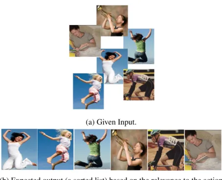
1.1 Image denoising and inpainting. . . 1 1.2 An example of action classification problem for the action class ‘jumping’.

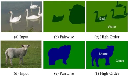
The ‘input’ is a set of bounding boxes. The desired ‘ouput’ is the sorted list in which all the bounding boxes with jumping action are ranked ahead of all the bounding boxes with non jumping action. Figure 1.2b shows one of the many possible outputs. . . 2 1.3 An illustration of the value of high-order interactions in solving segmentation

problems. Image source [67]. . . 6 1.4 Differences betweenAPand accuracy. The relevant class here is ‘jumping’.

The scores shown are obtained from the classifier. A positive score implies a relevant class (‘jumping’) and a negative score implies an irrelevant class (‘non jumping’). The bounding boxes are sorted based on the scores to obtain the ranking. An ideal ranking would have all the positive (or relevant) examples ahead of all the negative (irrelevant) ones. Notice that the accuracy is nothing but the fraction of misclassifications. . . 8 1.5 The example of high-order information in case of action classification. Notice

that people in the same image often perform the same action. This can be one of the hypotheses that encode meaningful high-order interactions. . . . 9 2.1 An example of handwritten word recognition. The input is an image of

a handwritten word x = {x1, x2, x3, x4}, where each xiis the bounding box

around each character of the word. The task is to predict the correct word, which in this case is ‘ROSE’. . . 14

2.2 Solution 1:Each bounding box is classified separately. The set of classes (or labels) is {a,··· ,z,A,··· ,Z}. The final solution is the collection of the predictions corresponding to each bounding box. The number of classifiers required is |L |(= 52), therefore, the solution is practically very efficient. However, it does not take account of the interdependencies between the output variables. . . 14 2.3 Solution 2:Each word is classified separately. The set of classes (or labels)

is {aaaa,··· ,zzzz,AAAA,··· ,ZZZZ}. Note that the number of prediction functions required is (52)4_{≈ 7 Million. Therefore, this solution is practically}

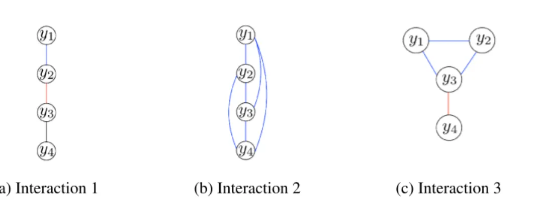
infeasible even for moderate length words. . . 15 2.4 Few examples of the different possible interactions between the output

variables. Variables in the edges with same colors form a clique. For example, in case of Figure 2.4c, set of cliques is: C = {c1, c2}, where c1= {y1, y2, y3}

and c2= {y3, y4}. Many other types of interactions are also possible. . . 17

2.5 The directed graph shown in Figure 2.5a is an example of an s-t Graph. All of the arc weights are assumed to be positive. In Figure 2.5b, the cost of Cut-1 is (w1+ w6+ w4), Vs is {s,v2}, Vt is {t,v1}, and the labeling is y = {1, 0}.

Similarly, the cost of Cut-2 is (w1+ w3), Vs is {s}, Vt is {t,v1, v2}, and the

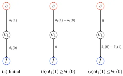
labeling is y = {1,1}. . . 24 2.6 The s-t graph construction for arbitrary unary potentials. Figure 2.6b shows

the s-t graph when the unary potential for label 1 is higher than that of label 0. Similarly, Figure 2.6b shows the s-t graph for the opposite case. Recall that a node in the set Vs and Vt is assigned the labels 0 and 1, respectively. . 26

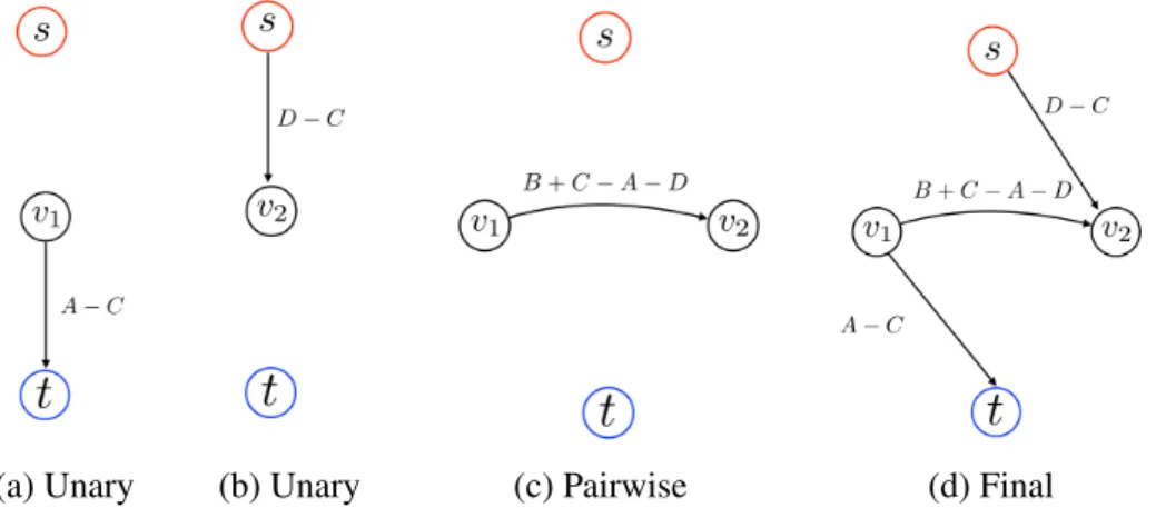
2.7 Graph construction for a given pairwise submodular energy for the case when A ≥ C and D ≥ C. Figures 2.7a and 2.7b are the graph constructions for θ1(0) = A −C and θ2(1) = D −C respectively. Figure 2.7c is the graph

construction for θ12(0, 1) = B +C − A − D. Figure 2.7d uses the additivity

theorem to construct the final graph. . . 27 2.8 An example of the move space for α−expansion with only four nodes in

the graph. Figure 2.8a shows the initial labeling from where the expansion move will take place. Figure 2.8b shows the possible labelings when α is the ‘Green’ label. Let the numbering of the nodes be in the clockwise manner starting from the top left corner. Then different binary vectors for all possible labelings are as follows: ta= {0, 0, 0, 0}, tb= {1, 0, 0, 0}, tc= {0, 0, 1, 0},

2.9 An example of the costs assigned by the Pn_{-Potts model. Let γ}

r, γb, and γg

be the costs for the colors ‘red’, ‘blue’, and ‘green’, respectively. γmax>

max(γr, γg, γb). Then the costs for the cases (a), (b), and (c) are all the same,

which is γmax. The cost for the case (d) is γg. . . 32

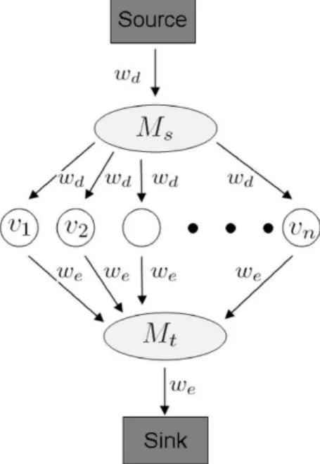
2.10 Graph construction for the Pn_{Potts model. M}

sand Mtare two auxiliary nodes.

The weights are wd= γ +k and we= γα+k, where, k = γmax−γα−γ. Figure

reproduced from [66]. . . 33 2.11 Pictorial representation of one iteration of theCCCP algorithm [138].

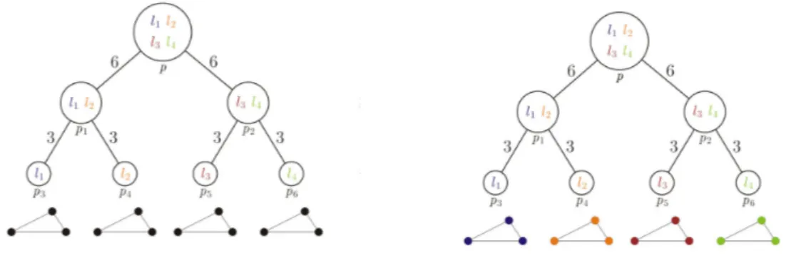
Fig-ure 2.11a shows the given difference of convex functions, which can be written as a sum of convex and concave functions. Figure 2.11b shows the linear upper bound for the concave function (−v(w)) at a given point, which results in an affine function ¯v(w). Finally, Figure 2.11c shows the resulting convex function as a sum of convex u(w) and affine ¯v(w) ones. . . 50 3.1 An example of r-HSTfor r= 2. The cluster associated with root p contains

all the labels. As we go down, the cluster splits into subclusters and finally we get the singletons, the leaf nodes (labels). The root is at depth of 1(τ = 1) and leaf nodes at τ = 3. The metric defined over the r-HST is denoted as dt(., .), the shortest path between the inputs. For example, dt_(l

1, l3) = 18

and dt(l1, l2) = 6. The diameter diversity for the subset of labels at cluster p

ismax_{{li,lj}∈{l1,l2,l3,l4}}dt(li, lj) = 18. Similarly, the diameter diversity at p2

and p3are 6 and 0, respectively. . . 64

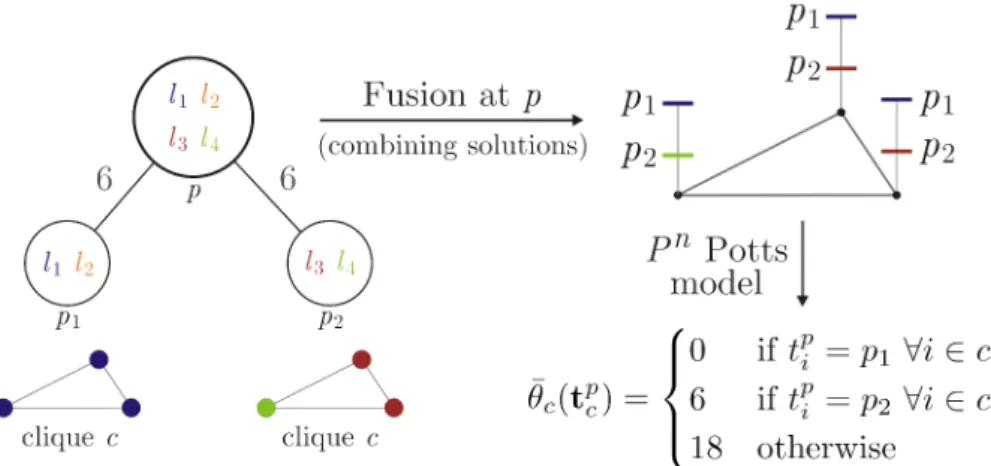
3.2 An example of solving the labeling problems at leaf nodes. Consider a clique with three nodes which we intend to label. Figure 3.2a shows the subprobelms at each leaf node. Notice that each leaf node contains only one label, therefore, we have only one choice for the labeling. Figure 3.2b shows the corresponding trivial labelings (notice the colors). . . 65 3.3 An example of solving the labeling problem at non-leaf node (p) by

combin-ing the solutions of its child nodes{p1, p2}, given clique c and the labelings

that it has obtained at the child nodes. The labeling fusion instance shown in this figure is the top two levels of the r-HSTin the Figure 3.1. Note that the labelings shown at nodes p1and p2are an assumption. It could get different

labelings as well but the algorithm for the fusion remains the same. The diameter diversity of the labeling of clique c at node p1is 0 as it contains

only one unique label l1. The diameter diversity of the labeling at p2 is

dt(l3, l4) = 6 and at p is max{li,lj}∈{l1,l3,l4}d

t_(l

i, lj) = 18. Please notice the

3.4 Synthetic (Blue: Our, Red: Co-occ [87]). The x-axis of all the figures is the weight associated with the cliques(wc). Figures (a) and (b) are the plots

when the hierarchical PnPotts model is known. Figures (c) and (d) are the plots when a diversity (diameter diversity over truncated linear metric) is given as the clique potentials which is then approximated using the mixture of hierarchical Pn Potts model. Notice that in both the cases our method outperforms the baseline [87] both in terms of energy and time. Also, for very high value of wc= 100, both the methods converges to the same labeling.

This is expected as a very high value of wc enforces rigid smoothness by

assigning everything to the same label. . . 76 3.5 Stereo Matching Results. Figures (a) and (d) are the ground truth disparity

for the ‘tsukuba’ and ‘teddy’ respectively. Our method significantly outper-forms the baseline Co-ooc [87] in both the cases in terms of energy. Our results are visually more appealing also. Figures (b) and (e) clearly shows the influence of ‘parsimonious labeling’ as the regions are smooth and the discontinuity is preserved. Recall that we use super-pixels obtained using the mean-shift as the cliques. . . 78 3.6 Comparison of all the methods for the stereo matching of ‘teddy’. We used

the optimal setting of the parameters proposed in the well known Middlebury webpage and [118]. The above results are obtained usingσ = 102for the Co-occ and our method. Clearly, our method gives much smooth results while keeping the underlying shape intact. This is because of the cliques and the corresponding potentials (diversities) used. The diversities enforces smoothness over the cliques while σ controls this smoothness in order to avoid over smooth results. . . 78 3.7 Comparison of all the methods for the stereo matching of ‘tsukuba’. We used

the optimal setting of the parameters proposed in the well known Middlebury webpage and [118]. The above results are obtained usingσ = 102for the Co-occ and our method. We can see that the disparity obtained using our method is closest to the ground truth compared to all other methods. In our method, the background is uniform (under the table also), the camera shape is closest to the ground truth camera, and the face disparity is also closest to the ground truth compared to other methods.. . . 79 3.8 Effect of σ in the parsimonious labeling. All the parameters are same except

for theσ . Note that as we increase the σ , the wcincreases, which in turn

3.9 Effect of clique size (superpixels). The top row shows the cliques (superpixels) used and the bottom row shows the stereo matching using these cliques. As we go from left to right, the minimum number of pixels that a superpixel must contain increases. All the other parameters are the same. In order to increase the weight wc, we use high value ofσ , which is σ = 105in all the

above cases. . . 79 3.10 Image inpainting results. Figures (a) and (d) are the input images of ‘penguin’

and ‘house’ with added noise and obscured regions. Our method, (b) and (e), significantly outperforms the baseline [87] in both the cases in terms of energy. Visually, our method gives much more appealing results. We use super-pixels obtained using the mean-shift as the cliques. . . 80 3.11 Comparison of all the methods for the image inpainting and denoising

problem of the ‘penguin’. Notice that our method recovers the hand of the penguin very smoothly. In other methods, except Co-oc, the ground is over-smooth while our method recovers the ground quite well compared to others. . . 80 3.12 Comparison of all the methods for the image inpainting and denoising

problem of the ‘house’. . . 81 4.1 Top 8 samples ranked by all the four methods for ‘reading’ action class. First

row –SVM, Second row –AP-SVM, Third row –HOB-SVM, and Fourth row –

HOAP-SVM. Note that, the first false positive is ranked 2nd in case ofSVM

(first row) and 3rd in case ofAP-SVM(second row), this shows the importance of optimizing the APloss. On the other hand, in case of HOB-SVM (third row), the first false positive is ranked 4th and the ‘similar samples’ (2nd and 3rd) are assigned similar scores, this illustrates the importance of using high-order information. Furthermore,HOAP-SVM (fourth row) has the bestAP

among all the four methods, this shows the importance of using high-order information and optimizing the correct loss. Note that, in case ofHOAP-SVM, the 4th and 5th ranked samples are false positives (underlying action is close to reading) and they both belong to the same image (our similarity criterion). This indicates that high-order information sometimes may lead to poor testAPin case of confusing classes (such as ‘playinginstrument’ vs ‘usingcomputer’) by assigning all the connected samples to the wrong label.

5.1 In each figure, x-axis is the λ and y-axis is the number of passes. In case of regularization path algorithms (starting with RP), x-axis represents all the

breakpoints for the entire path, and y-axis represents the number of passes required to reach κ1ε optimal solution at each breakpoint (warm start with ε

optimal solution). In other two algorithms (no regularization path), x-axis represents 20 values of λ evenly spaced in the range of [10−4_{, 10}3_{], and}

y-axis represents the number of passes to reach ε optimal solution (initialization with w = 0). . . 135 5.2 Figure 5.2a shows the ‘legend’ for the purpose of clarity. In all other figures,

x-axis is the λ and y-axis is the duality gap. In case of regularization path algorithms (starting with RP), x-axis represents all the breakpoints for the

entire path. In other two algorithms (no regularization path), x-axis represents 20 values of λ evenly spaced in the range of [10−4_{, 10}3_{]. Recall that in case}

of regularization path algorithms the solution we seek must be κ1ε optimal. 136

5.3 In all figures, x-axis is the λ and y-axis is the test loss. In all the experiments, the test losses are obtained for models corresponding to 20 different values of λ equally spaced in the range of [10−4_{, 10}3_{]. . . 137}

A.1 The top row represents the sample slices from three different volumes of the RT Parotids dataset. The middle row represents the sample slices of the RT Abdominal dataset, and the last row represents the sample slices from the IBSR dataset. . . 156 A.2 Overlapping of the segmentation masks in different views for one registration

case from RT Abdominal (first and second rows) and RT Parotids (third and fourth rows) datasets. The first column corresponds to the overlapping before registration between the source (in blue) and target (in red) segmen-tation masks of the different anatomical structures. From second to sixth column, we observe the overlapping between the warped source (in green) and the target (in red) segmentation masks, for the multiweight algorithm (MW) and the single metric algorithm usingSAD,MI,NCCand DWT). We

observe thatMWgives a better fit between the deformed and ground truth

structures than the rest of the single similarity measures, which are over segmenting most of the structures showing a poorer registration performance. 157

A.3 Qualitative results for one slice of one registration case from IBSR dataset. Since showing overlapped structures in the same image is too ambiguous given that the segmentation masks almost cover the complete image, we are showing the intensity difference between the two volumes. The first column shows the difference of the original volumes before registration. From second to sixth column we observe the difference between the warped source and the target images, for the MWand the single metric algorithm

usingSAD,MI,NCCorDWT). According to the scale in the bottom part of

the image, extreme values (which mean high differences between the images) correspond to blue and red colors, while green indicates no difference in terms of intensity. Note how most of the big differences observed in the first column (before registration) are reduced by theMW algorithm, while some

of them (specially in the peripheral area of the head) remain when using single metrics. . . 158 A.4 Results for the RT parotids dataset for the single-metric registration (SAD,

MI, NCC, DWT) and the multi-metric registration (MW). The weights for

the multi-metric registration are learned using the framework proposed in this work. ‘Parotl’ and ‘Parotr’ are the left and the right organs. The red square is the mean and the red bar is the median. It is evident from the results that using the learned linear combination of the metrics outperforms the single-metric based deformable registration. . . 159 A.5 Results for the RT abdominal dataset for the single-metric registration (SAD,

MI, NCC, DWT) and the multi-metric registration (MW). The weights for

the multi-metric registration are learned using the framework proposed in this work. ‘Bladder’, ‘Sigmoid’, and ‘Rectum’ are the three organs on the dataset. The red square is the mean and the red bar is the median. It is evident from the results that using the learned linear combination of the metrics outperforms the single-metric based deformable registration. . . 160 A.6 Results for the IBSR dataset for the single-metric registration (SAD, MI,

NCC, DWT) and the multi-metric registration (MW). The weights for the

multi-metric registration are learned using the framework proposed in this work. ‘CSF’, ‘Grey Mater’, and ‘White Mater’ are different structures in the brain. The red square is the mean and the red bar is the median. It is evident from the results that using the learned linear combination of the metrics outperforms the single-metric based deformable registration. . . 161

B.1 The blue curve shows the convex function and the black polygon shows the convex compact domain. At a given qk, the Figure B.1a shows the

linearization and the minimization of the linearized function over the domain to obtain the atom sk. Figure B.1b shows the new point qk+1 obtained using

the linear combination of qk and sk. The green line shows the linearization

at the new point qk+1, and sk+1 is the new atom obtained as a result of the

minimization of this function. . . 168 B.2 Visualization of the linearization duality gap. The blue curve is the convex

function f . The red line is the linearization of f at qk, denoted as fl. The

atom s is obtained as the result of the minization of flover the domain. The

4.1 The AP over five folds for the best setting of the hyperparameters obtained using the cross-validation. Our frameworks outperformsSVMandAP-SVM

in all the 10 action classes. Note thatHOAP-SVMis initialized withHOB-SVM.101

4.2 The AP of all the four methods. The training is performed over the entire ‘trainval’ dataset of PASCAL VOC 2011 using the best hyperparameters obtained during 5-fold cross-validation. The testing is performed on the ‘test’ dataset and evaluated on the PASCAL VOC server. Note thatHOAP-SVMis initialized usingHOB-SVM. . . 101 5.1 No regularization path: Initialization with w = 0. We used 20 different values

of λ equally spaced in the range of [10−4_{, 10}3_{] and four variants of theBCFW}

algorithm. Total passes represents the total number of passes through the entire dataset using all the 20 values of λ . Min test loss represents the minimum value of the test loss obtained by using all the 20 trained models. Clearly, the gap based sampling method (BCFW-STD-G) requires less number

of passes to achieve the same generalization. . . 131 5.2 Regularization path: κ1vs total passes for four different variants of theBCFW

algorithm.The total passes represents the total number of passes through the entire dataset to obtain the complete regularization path. . . 131 5.3 Regularization path: κ1 vs number of regularization parameters (λ ) for

four different variants of the BCFW algorithm. The number of

regulariza-tion parameters is basically the number of kinks that divide the complete regularization space into segments. . . 131

5.4 Regularization path: κ1 vs minimum test loss. For a given regularization

path, the test losses are obtained for models corresponding to 20 different values of λ equally spaced in the range of [10−4_{, 10}3_{] (same as in case of no}

regularization path experiments). Notice that the models are trained using the regularization path algorithm. For each path, the minimum test loss is the minimum over the 20 different values. . . 132

Introduction

The main focus of this thesis is to develop high-order inference and machine learning algorithms to process visual and medical data in order to extract useful information. We begin with two challenging tasks in order to develop intuition about the need for inference and learning algorithms. The first task that we consider is image denoising and inpainting as shown in the Figure 1.1. Given an image with added noise and obscured regions (regions with missing pixels) as shown in Figure 1.1a, the problem is to automatically denoise the image and fill the obscured regions such that it is consistent with the surrounding. Another task under consideration is ‘learning to rank’. We give an example of the learning to rank task in the context of action classification as shown in Figure 1.2. Given a set of bounding boxes (refer Figure 1.2a), the task is to find an ordering of the bounding boxes based on their relevance with respect to a given action class such as ‘jumping’.

(a) Given Input. (b) Expected Output.

Figure 1.1: Image denoising and inpainting.

Let us first try to understand the complexity of the first task. Assume that the input image is gray scale of resolution m × n. Therefore, each pixel in the image can be assigned any integer value in the range [0,255]. In the simplest possible case, we assume that each pixel is independent of any other pixel in the image. Therefore, the denoising task can be solved

(a) Given Input.

(b) Expected output (a sorted list) based on the relevance to the action class ‘jumping’.

Figure 1.2: An example of action classification problem for the action class ‘jumping’. The ‘input’ is a set of bounding boxes. The desired ‘ouput’ is the sorted list in which all the bounding boxes with jumping action are ranked ahead of all the bounding boxes with non jumping action. Figure 1.2b shows one of the many possible outputs.

by processing each pixel independently. For example, thresholding based on some criterion such as average intensity value of the image pixels. This approach is computationally highly efficient as it requires only N = m × n operations. However, it is of little practical value for the following two reasons: (i) individually processing each pixel will not lead to a contextually meaningful output; and (ii) local information is not sufficient to solve the inpainting problem. Therefore, in order to get a meaningful solution, we must take into account the interdependencies between the pixels. Since each pixel can be assigned 256 possible values (also called labels), considering the interdependencies leads to a problem with (256)N _{possible combinations (or solutions), a much harder problem to solve. Finding}

the best solution out of these exponentially many possible combinations is known as the inferenceproblem. In the case of vision related problems, inference involves thousands or sometimes millions of interdependent variables, which makes it very hard to solve. Normally, possible solutions are evaluated using a mathematical energy function that assigns a score to each possible solution. The solution corresponding to the minimum score is considered to be the optimal solution. In general, energy minimization problem isNP-HARD. However,

specialized and highly efficient algorithms. Some successful examples of such inference algorithms are graph cuts [74], belief propagation [105], and α-expansion [128]. A detailed discussion of these algorithms is given in chapter 2. They are very useful in many tasks such as semantic segmentation, pose estimation, stereo reconstruction, image inpainting, image registration, and many more. In this thesis, we develop a new family of high-order inference problems which we call parsimonious labeling, and propose very efficient algorithms for their optimization along with strong theoretical guarantees.

Now consider the ‘learning to rank’ task (Figure 1.2). Given a set of bounding boxes, the task is to rank them based on their relevance with respect to an action class such as ‘jumping’. The quality of the ranking is evaluated based on a user defined metric such as average precision (a standard measure of the quality of a ranking). Let us assume that we are given a parametric energy function (similar to the previous example) which assigns a score to each bounding box. Given such scores, ranking reduces to sorting the bounding boxes based on their scores. Hence, the quality of the ranking depends entirely on the scores assigned to the bounding boxes by the energy function, which in turn depend on the parameters of the energy function. So in order to obtain scores that lead to high average precision, the parameters of the energy function must be chosen carefully. Normally, the energy function contains thousands of parameters and hand tuning these parameters is practically infeasible. In order to circumvent this problem, the standard approach is to learn the parameters values using sophisticated machine learning techniques1. In this thesis, we develop new machine learning methods for solving tasks that produce rankings as their final outcome. On top of this, we develop a new algorithm for the regularization path for structuredSVM, that allows us to obtain the best

possible mapping function in tasks that can be modeled using the well known structuredSVM

framework.

In the following sections, we briefly discuss the importance, complexity, and challenges of inference, machine learning (for ranking), and regularization path algorithms, then provide an outline of the thesis followed by the list of publications where the work in this thesis has previously appeared.

1_{Machine learning is the field of study that allows computers to learn from experiences. It evolved with}

time as a highly useful and effective blend of different fields such as computational statistics, mathematical optimization, and graph theory. More precisely, machine learning is the task of estimating a mapping function of the objects that we want to predict. In general supervised setting, a training data for which the prediction is known is used to learn this mapping. Few examples of highly successful applications of machine learning are search engines, character/voice recognition, spam filtering, news clustering, recommender systems, object classification, automatic language translation, and many more.

1.1

High-Order Inference

As discussed earlier, inference problem can involve thousands or millions of interdependent variables with solution spaces that are exponentially large in this number. To encode the semantics of the problem, we define a mathematical function known as the energy function that quantifies the quality of each possible solution. The solution with the lowest energy is the optimal choice. Mathematically, consider a random field defined over a set of random variables y = {y1, · · · , yN}, each of which can take a value from a discrete label set L =

{l1, · · · , lH}. Furthermore, let C denote the set of maximal cliques that characterize the

interactions between these variables. Each clique consists of a set of random variables that are connected to each other in the lattice. For example, in case of image denoising problem, the set of random variables are the pixels in the image, N = m × n, and the label set is L _{= {0, · · · , 255}. To assess the quality of each output (or labeling) y we define an energy} function as: E(y) =

_∑

∑

where θi(yi) is the unary potential for assigning a label yi to the i-th variable, and θc(yc)

is the clique potential for assigning the labels ycto the variables in the clique c. Once we

have such a function, we need a method to evaluate each possible assignment in order to find the best one. The exhaustive search is practically infeasible. For example, in case of image denoising, if m = n = 100, then there are (256)10,000 _{possible outcomes. One approach}

to solve this task is to use inference algorithms where we need to model the problem in a restricted yet useful setting to which a computationally efficient algorithm can be devised to find the optimal assignment among the exponentially many. Broadly speaking, there are two major steps to solving such inference problems: (i) modeling – selecting a suitable but tractable energy function (discussed in detail in chapter 2); (ii) optimization – finding the solution corresponding to the minimum energy (inference algorithm). The two steps goes hand-in-hand. Normally, we model the problem in such a manner that an algorithm can be devised to optimize it in polynomial time. Modeling defines restrictions on the potentials, interactions among the random variables (pixels in case of images), and optimality conditions for the inference algorithm. There are several situations in which careful modeling allows us to optimize the problem very efficiently. Let us have a quick look into some of these modeling strategies and their corresponding optimization algorithms.

• Restricting the potentials: In case the clique potentials are restricted to be submod-ular distance functions over the labels [1, 47], an optimal solution of the inference

problem can be computed in polynomial time by solving an equivalent Graph cut problem [112]. A special case of this with two labels is well addressed in the seminal work [74]. Of course, restricting the potentials limits our modeling capabilities. How-ever, submodular potential functions provide smoothness which is a desired property for many important tasks such as binary image restoration [14, 15, 51, 57], foreground background segmentation [13], medical image segmentation [11, 12], stereo depth recovery [14, 15, 56], and many other tasks.

• Restricting the structure: If the interactions between the random variables are re-stricted to form a tree (graph with no cycles), then the well known belief propagation method [105] can be used to obtain the globally optimal solution of the inference problem in polynomial time. Tree structures can still encode rich interactions useful to many vision tasks such as ‘pose estimation’ [134] and ‘object detection’ [34].

• Compromising on optimality: Sometimes it is not possible to obtain the globally optimal solution to the problem. In such situations, algorithms are designed to obtain a good local minimum with theoretical guarantees (multiplicative bounds). One example of such algorithm is the well known α−expansion [15, 128] which obtains good local minima for problems in which the clique potential is a metric distance function over the labels.

The above mentioned algorithms are known to work well for pairwise interactions. However, higher order cliques (ones with more than two random variables) can model richer and more meaningful context, and have proven to be very useful in many vision tasks. one example representing the advantages of higher order interactions is shown in the Figure 1.3. However as the size of the cliques increases, the complexity of inference increases. Modeling and optimizing higher order energy functions is a highly challenging task. Technical restrictions on the clique potentials allows us to devise efficient algorithms for many high order problems. For example, the Pn_{-Potts model [66], label-cost based potential functions [28], and}

Co-occurrence statistics based potential functions [87]. Below we highlight two main challenges for devising inference problems over graphs with high order cliques.

Challenges.

• Defining new family of higher order clique potentials: The known families of higher order clique potentials are either too restrictive with limited modeling capabilities or their optimization algorithms are inefficient and do not provide good local minima with theoretical guarantees. Therefore, it is challenging to define new sets of clique

potentials with higher modeling capabilities that are useful for vision tasks and that support efficient optimization algorithms. For example, parsimony is a desirable property for many vision tasks. Parsimony refers to using fewer labels, which in turn provides smoothness. On one hand, the Pn_{-Potts model provides parsimony but it is}

too rigid and sometimes gives over-smooth results. On the other hand, Co-occurrence statistic based potential functions [87] are much more expressive but their optimization algorithm does not provide any theoretical guarantees.

• Proposing efficient algorithms with theoretical guarantees: As discussed earlier, for a given family of high order clique potential functions, it is a challenging task to provide efficient algorithms for the optimization. For example, the SoSPD [40] allows us to use arbitrary clique potentials, but its optimization algorithm is practically inefficient and is not advisable to use beyond cliques of size ten. Similarly, Co-occurrence statistic based potential functions [87] allow us to use clique potentials that encode parsimonyand their optimization is efficient, allowing larger cliques (beyond clique size of 1200). However, the optimization algorithm of [87] does not provide any theoretical guarantees, thus, the local minima obtained may or may not be useful.

(a) Input (b) Pairwise (c) High Order

(d) Input (e) Pairwise (f) High Order

Figure 1.3: An illustration of the value of high-order interactions in solving segmentation problems. Image source [67].

1.2

Learning to Rank

Many computer vision tasks require the development of automatic methods that sort or rank a given set of visual samples according to their relevance to a query. For example, consider

the problem of action classification (or more precisely action ranking). The input is a set of samples corresponding to bounding boxes of persons, and an action such as ‘jumping’. The desired output is a ranking where a sample representing a jumping person is ranked higher than a sample representing a person performing a different action. An example of such problem is shown in the Figure 1.2. Other related problems include image classification (sorting images according to their relevance to a user query) and object detection (sorting all the windows in a set of images according to their relevance to an object category). Once the ranking is obtained, it can be evaluated using average precision (AP), which is a widely used

measure of the quality of a ranking. The most common approach of solving this problem is to train a binary classifier (often a support vector machine (SVM)). SVM optimizes an

upper bound on an accuracy based loss function to learn a parameter vector. At test time, the learned parameter vector is used to assign scores (confidence of being relevant) to each sample. The samples are then sorted based on these scores to get the final ranking. However, this approach suffers from following two drawbacks. First, average precision and accuracy are not the same measures. Figure 1.4 shows some examples whereAP and accuracy are

different. It is clear from these examples that a classifier that provides high accuracy may not give high average precision. In another words, optimizing accuracy may result in suboptimal average precision. Therefore, in a situation where the desired result is a ranked list, it is better to optimize an average precision based loss function (a measure of the quality of the ranking). Unfortunately, unlike accuracy based loss function, as used inSVM, the average

precision is non decomposable and thus hard to optimize. AP-SVM[137] poses the problem

as a special case of structuredSVMand provides efficient algorithm for optimizing an upper

bound on average precision based loss function. The second drawback is thatSVMcan use

only first order information. Whereas there is a great deal of high order information in many vision related tasks (and other tasks as well). For example, in action classification, people in the image are often performing same action (see Figure 1.5 for a few examples). In object detection, objects of the same category tend to have similar aspect ratios. In pose estimation, people in the same scene tend to have similar poses (e.g. sitting down to watch a movie). In document retrieval, documents containing the same or similar words are more likely belong to the same class. Therefore, we need to use richer machine learning frameworks such as structuredSVM, that are capable of encoding the high order interactions.

Challenge. The challenge lies in developing a framework capable of optimizing average precision while using high order information. On the one hand, a special case of the structured

SVM(AP-SVM) can optimize average precision based loss functions, but it does not allow us

(a)AP/Acc = 1.0/1.0

(b)AP/Acc = 1.0/0.83

(c)AP/Acc = 0.55/0.66

Figure 1.4: Differences between AP and accuracy. The relevant class here is ‘jumping’.

The scores shown are obtained from the classifier. A positive score implies a relevant class (‘jumping’) and a negative score implies an irrelevant class (‘non jumping’). The bounding boxes are sorted based on the scores to obtain the ranking. An ideal ranking would have all the positive (or relevant) examples ahead of all the negative (irrelevant) ones. Notice that the accuracy is nothing but the fraction of misclassifications.

order information, it only allows us to optimize accuracy based (or similar but decomposible) loss functions.

1.3

Regularization Path

In the previous section we talked about StructuredSVMtype frameworks for learning tasks.

The objective function of an SSVMis parametric, depends on a particular regularization

parameter λ (also referred as C, inversely proportional to λ ), which controls the trade-off between the model complexity and an upper bound on the empirical risk (detailed in chapter 2). The value of the regularization parameter has a significant impact on the performance and the generalization of the learning method. Thus, we must choose it very carefully in order to obtain the best model. Finding an appropriate value for the regularization parameter often requires us to tune it, but lack of knowledge about the structure of the regularization problem compels us to cross validate it over the entire parameter space, which

Figure 1.5: The example of high-order information in case of action classification. Notice that people in the same image often perform the same action. This can be one of the hypotheses that encode meaningful high-order interactions.

is practically infeasible owing to its computational cost. To circumvent this, the standard approach is to resort to a sub optimal solution by cross validating a small set of regularization parameter values on a given training dataset. Doing this is tedious and quickly becomes infeasible as we increase the number of regularization values tested. Therefore, we need an efficient algorithm to obtain the entire regularization path of SSVM. By definition the

regularization path is the set of solutions for all possible values of the regularization parameter in the parameter space [29]. Obtaining the regularization path for any parametric model implies exploring the whole regularization parameter space in a highly efficient manner to provide the optimal learned model for any given value of λ ∈ [0,∞]. This allows us to efficiently obtain the best possible model. The key idea behind the algorithm is to break the regularization parameter space into segments such that learning an ε-optimal model for any value of λ in a given segment guarantees that the same learned model is ε-optimal for all values of λ in the segment.

Challenges.

• Finding the segments (or the breakpoints): As mentioned earlier, the idea behind regularization path is to break the regularization parameter space λ ∈ [0,∞] into segments. This can be achieved by finding breakpoints or kinks such that if the learned model is ε-optimal for any λ ∈ [λk, λk−1), then it is ε-optimal for all λ ∈ [λk, λk−1).

One of the challenge is to find these breakpoints in an efficient manner. The other challenge is to reduce the needed number of breakpoints.

• Efficiently optimizing at each breakpoint: Each breakpoint defines a new segment. Therefore, at each breakpoint we need to update (optimize) the learned model so that it is ε-optimal for the given segment. In order to make this practically feasible, we must devise an algorithm that can be warm-started using the solution of the previous segment for faster convergence.

1.4

Thesis Outline

Chapter 2 is a review of structuredSVMand related inference algorithms. Specifically, we

discuss theSSVMalgorithm with examples, various inference algorithms such as graph cuts,

α-expansion, metric labeling, and Pn_{-Potts model, and different optimization algorithms for} SSVM. Finally, we talk about latentSSVMand the corresponding concave-convex procedure

for the problems related to the weakly supervised settings.

In chapter 3, we describe a new family of inference problems that we call parsimonious labeling, which handle all the challenges discussed in section 1.1. Parsimonious labeling can be seen as a high order extension of the famous metric labeling problem. We also propose the hierarchical Pn_{-Potts model and show how parsimonious labeling can be modeled as a}

mixture of hierarchical Pn_{-Potts models. Finally, we propose an efficient algorithm with}

strong theoretical guarantees for the optimization of parsimonious labelings and show its efficacy on the challenging tasks of stereo matching and image in-painting.

In chapter 4, we propose a new learning framework, High-Order Average Precision SVM (HOAP-SVM), capable of optimizing average precision while using high-order information

(see the challenges discussed in section 1.2). We show the efficacy ofHOAP-SVMon the task

of action classification.

In chapter 5, we present a new algorithm (SSVM-RP) to obtain ε-optimal regularization paths

forSSVM. We propose intuitive variants of the Block-Coordinate Frank-Wolfe algorithm for

the faster optimization ofSSVM-RP. In addition to this, we propose a principled algorithm

for optimizingSSVM with additional box constraints. Finally, we propose a regularization

path algorithm forSSVM with additional positivity/negativity constraints. All the research

presented in this chapter were conducted under the supervision of Dr. Simon Lacoste-Julien at the SIERRA Team of INRIA (Paris) during my visit from15th June 2015 to15th September 2015.

Finally, in appendix A, we present a novel weakly supervised algorithm for learning context specific metric aggregations for the challenging task of 3D-3D deformable registration. We demonstrate the efficacy of our framework using three challenging datasets related to medical imaging.

1.5

List of publications

Published in International Conferences and Journals

1. Learning-Based Approach for Online Lane Change Intention Prediction; Puneet Kumar, M. Perrollaz, S. Lefevre, C. Laugier; In IEEE Intelligent Vehicle Symposium (IV) 2013.

2. Discriminative parameter estimation for random walks segmentation; P. Y. Baudin, D. Goodman, P. K. Dokania , N. Azzabou, P. G. Carlier, N. Paragios, M. Pawan Kumar; In MICCAI 2013.

3. Learning to Rank using High-Order Information; P. K. Dokania, A. Behl, C. V. Jawahar, M. P. Kumar; In ECCV 2014.

4. Parsimonious Labeling; P. K. Dokania, M. P. Kumar; In ICCV 2015.

5. Partial Linearization based Optimization for Multi-class SVM; P. Mohapatra, P. K. Dokania, C. V. Jawahar, M. P. Kumar; In ECCV 2016.

6. Minding the Gaps for Block Frank-Wolfe Optimization of Structured SVMs; A. Osokin, JB Alayrac, I. Lukasewitz, P. K. Dokania, S. Lacoste-Julien; In ICML 2016.

7. Rounding-based Moves for Semi-Metric Labeling; M. P. Kumar, P. K. Dokania; In JMLR 2016.

Under Submission

1. Deformable Registration through Learning of Context-Specific Metric Aggregation; E. Ferrante, P. K. Dokania2_{, N. Paragios.}

Review of Structured SVM and related

Inference Algorithms

2.1

Motivation

Structured output prediction [88, 122, 126] is one of the key problems in the machine learning and computer vision community. It deals with learning a function f that maps the input space X (patterns or vectors) to a complex output space Y (graphs, trees, strings, or sequences). In other words, structured prediction is the problem of learning prediction functions that take into account the interdependencies among the output variables. In order to give better insight into the problem of structured prediction, we consider the task of recognizing handwritten words [63]. An example is shown in Figure 2.1. The problem is to predict the word given bounding boxes around letters. Below we discuss two possible solutions to this problem (from a discriminative classification point of view) and progressively build intuition to understand the complexity and importance of structured prediction. Before discussing the solutions, we define some notation for the purpose of clarity. We denote the number of letters in the word as p. In our example, p = 4. The input, which in this case is a collection of segmented bounding boxes in an image, is represented as x = {x1, x2, x3, x4}, where xi

denotes the i-th box. Similarly, we define the output, which is a word, as a collection of letters y = {y1, y2, y3, y4} ∈ Y . Here each output variable can be assigned any letter from the

alphabet. In other words, yi∈ L = {a, · · · , z, A, · · · , Z} for all i ∈ {1, 2, 3, 4}. Thus, the final

output space is Y = Lp_{, where p = 4. For example, for the input image in the Figure 2.1,}

the ground truth output is ‘ROSE’, therefore, y1= R, y2= O, y3= S, and y4= E. Using this