HAL Id: hal-00783198
https://hal.inria.fr/hal-00783198v2
Submitted on 5 Feb 2013
HAL is a multi-disciplinary open access
archive for the deposit and dissemination of
sci-entific research documents, whether they are
pub-lished or not. The documents may come from
teaching and research institutions in France or
L’archive ouverte pluridisciplinaire HAL, est
destinée au dépôt et à la diffusion de documents
scientifiques de niveau recherche, publiés ou non,
émanant des établissements d’enseignement et de
recherche français ou étrangers, des laboratoires
Grids with Interferences
Jean-Claude Bermond, Bi Li, Nicolas Nisse, Hervé Rivano, Min-Li Yu
To cite this version:
Jean-Claude Bermond, Bi Li, Nicolas Nisse, Hervé Rivano, Min-Li Yu. Data Gathering and
Person-alized Broadcasting in Radio Grids with Interferences. [Research Report] RR-8218, INRIA. 2013.
�hal-00783198v2�
0249-6399 ISRN INRIA/RR--8218--FR+ENG
RESEARCH
REPORT
N° 8218
January 2013Personalized
Broadcasting
in Radio Grids with
Interferences
RESEARCH CENTRE
SOPHIA ANTIPOLIS – MÉDITERRANÉE
2004 route des Lucioles - BP 93
Jean-Claude Bermond
∗, Bi Li
∗ †, Nicolas Nisse
∗, Hervé Rivano
‡,
Min-Li Yu
§Project-Teams Coati
Research Report n° 8218 — January 2013 — 34 pages
This work is partially supported by APRF RAISOM (PACA & FEDER), Project STREP FP7 EULER, ANR Verso project Ecoscells and ANR GRATEL.
∗Coati Project, INRIA–I3S(CNRS/UNSA), Sophia Antipolis, France
†Institute of Applied Mathematics, Chinese Academy of Sciences, Beijing, China ‡SWING, INRIA Rhônes Alpes and CITI Lab (INSA Lyon), Lyon, France
Moreover, the communication is subjet to interference constraints, more precisely, two calls interfere in a step, if one sender is at distance at most dI from the other caller. Given a graph with a base station and
a set of nodes having some messages, the goal of the gathering problem is to compute a schedule of calls for the base station to receive all messages as fast as possible, i.e., minimizing the number of steps (called makespan). The gathering problem is equivalent to the personalized broadcasting problem where the base station has to send messages to some nodes in the graph, with same transmission constraints.
In this paper, we focus on the gathering and personalized broadcasting problem in grids. Moreover, we consider the non-buffering model: when a node receives a message at some step, it must transmit it during the next step. In this setting, though the problem of determining the complexity of computing the optimal makespan in a grid is still open, we present linear (in the number of messages) algorithms that compute schedules for gathering with dI ∈ {0, 1, 2}. In particular, we present an algorithm that achieves the optimal
makespan up to an additive constant 2 when dI = 0. If no messages are “close" to the axes (the base station
being the origin), our algorithms achieve the optimal makespan up to an additive constant 1 when dI = 0,
4 when dI = 2, and 3 when both dI = 1 and the base station is in a corner. Note that, the approximation
algorithms that we present also provide approximation up to a ratio 2 for the gathering with buffering. All our results are proved in terms of personalized broadcasting.
Résumé : Dans le problème de la collecte, un sommet particuler (la base) doit recevoir des messages de certains sommets dans un graphe. A chaque étape, un nœud peut envoyer un message à un de ses voisins. De plus, les communications sont sujettes à des interférences. Le but du problème est de calculer l’ordre des envois pour que la base reçoive tous les messages aussi vite que possible. Le nombre d’étapes d’un ordre est le makespan. Le problème de collecte est équivalent au problème de diffusion personnalisée où la base doit envoyer des messages personnalisés à certains des sommets du graphe, avec les mêmes contraintes d’interférence. Dans cet article, nous considérons ces problèmes dans les grilles et dans le cas où le buffering n’est pas permis. La complexité de calculer le makespan minimum n’est pas connue dans le case des grilles. Nous proposons des algorithmes, pour les cas d’interférences à distance dI ∈ {0, 1, 2},
pour calculer des ordres acceptables (sans collisions de messages) en temps linéaire en le nombre de messages. Nos algorithmes calculent des ordres dont le makespan est à une petite constante de l’optimal. Lorsqu’aucun message n’a une destination “proche" des axes (la base étant l’origine), il s’agit d’une +1 approximation dans le cas dI = 0, d’une +4 approximation dans le cas dI = 2, et, si de plus la base est un
coin de la grille, d’une +3 approximation dans le cas dI = 1. Nous prouvons aussi que nos algorithmes
sont des approximations avec facteur multiplicatif 2 dans le cas où le buffering est autorisé. Nos résultats améliorent des résultats connus dans la litérature et sont prouvés en termes de diffusion personnalisée. Mots-clés : calcul formel, base de formules, protocole, différentiation automatique, génération de code, modélisation, lien symbolique/numérique, matrice structurée, résolution de systèmes polynomiaux
1
Introduction
1.1
Problem, model and assumptions
In this paper, we study a problem that was motivated by designing efficient strategies to provide internet access using wireless devices [8]. Typically, several houses in a village need access to a gateway (for example a satellite antenna) to transmit and receive data over the Internet. To reduce the cost of the transceivers, multi-hop wireless relay routing is used. We formulate this problem as gathering information in a Base Station (denoted by BS) of a wireless multi-hop network when interferences constraints are present. This problem is also known as data collection and is particularly important in sensor networks and access networks.
Transmission model We adopt the network model considered in [2, 4, 9, 11, 16]. The network is represented by a node-weighted symmetric digraph G = (V, E), where V is the set of nodes and E is the set of arcs. More specifically, each node in V represents a device (sensor, station, . . . ) that can transmit and receive data. There is a special node BS ∈ V called the Base Station (BS), which is the final destination of all data possessed by the various nodes of the network. Each node may have any number of pieces of information, or messages, to transmit, including none. There is an arc from u to v if u can transmit a message to v. We suppose that the digraph is symmetric; so if u can transmit a message to v, then v can also transmit a message to u. Therefore G represents the graph of possible communications. Some authors use an undirected graph (replacing the two arcs (u, v) and (v, u) by an edge {u, v}). However calls (transmissions) are directed: a call (s, r) is defined as the transmission from the node s to node r, in which s is the sender and r is the receiver and s and r are adjacent in G. The distinction of sender and receiver will be important for our interference model.
Here we will consider grids as they model well both access networks and also random networks [14]. We assume that the time is slotted and that during each time slot, or step a transmission or a call between two nodes can transport at most one message. The network is assumed to be synchronous. We suppose that each device is equipped with an half duplex interface: a node cannot both receive and transmit during a step. This models the near-far effect of antennas: when one is transmitting, it’s own power prevents any other signal to be properly received.
Following [11, 12, 15, 16, 18] we assume that no buffering is done at intermediate nodes and each node forwards a message as soon as it receives it. One of the rationales behind this assumption is that it frees intermediate nodes from the need to maintain costly state information and message storage. Interference model We use a binary asymmetric model of interference based on the distance in the communication graph. Let d(u, v) denote the distance, that is the length of a shortest directed path, from u to v in G and dI be an nonnegative integer. We assume that when a node u transmits, all nodes v
such that d(u, v) ≤ dI are subject to the interference from u’s transmission. We assume that all nodes
of G have the same interference range dI. Two calls (s, r) and (s0, r0) do not interfere if and only if
d(s, r0) > dI and d(s0, r) > dI. Otherwise calls interfere (or there is a collision). We will focus on the
cases when dI ≤ 2. Note that, if dI > 0, the interference constraints include the fact that a node cannot
simultaneously send and receive messages. On the other hand, if dI = 0, the only constraint is that a
node cannot receive and send simultaneously, and it can send or receive at most one message per step. These hypotheses are strong and under the assumption of a centralized view. Moreover the binary interference model is a simplified version of the reality, where the Signal-to-Noise-and-Interferences Ratio (the ratio of the received power from the source of the transmission to the sum of the thermic noise and the received powers of all other simultaneously transmitting nodes) has to be above a given threshold for a transmission to be successful. However, the values of the completion times that we obtain will give lower bounds on the corresponding real life values. Stated differently, if the value of the completion time
is fixed, then our results will give upper bounds on the maximum possible number of users ( or messages that can be transmitted) in the network.
Gathering and Personalized broadcasting Our goal is to design protocols that will efficiently, i.e., quickly, gather all messages to the base station BS subject to these interference constraints. More for-mally, let G = (V, E) be a connected symmetric digraph, BS ∈ V and and dI ≥ 0 be an integer. Each
node in V \ BS is assigned a set (possibly empty) of messages that must be sent to BS. The gather-ing problem consists in computing a multi-hop schedule for each message to arrive the BS under the constraint that during any step any two calls do not interfere within the interference range dI. The
com-pletion time or makespan of the schedule is the number of steps used for all messages to reach BS. We are interested in computing the schedule with minimum makespan.
Actually, we will describe the gathering schedule by illustrating the schedule for the equivalent per-sonalized broadcasting problemsince this formulation allows us to use a simpler notation and simplify the proofs. In this problem, the base station BS has initially a set of personalized messages and they must be sent to their destinations, i.e., each message has a personalized destination in V , and possibly several messages may have the same destination. The problem is to find a multi-hop schedule for each message to reach its corresponding destination node under the same constraints as the gathering problem. The completion time or makespan of the schedule is the number of steps used for all messages to reach their destination and the problem aims at computing a schedule with minimum makespan. To see that these two problems are equivalent, from any personalized broadcasting schedule, we can always build a gathering schedule with the same makespan, and the other way around. Indeed, consider a personalized broadcasting schedule with makespan T . Any call (s, r) occurring at step k corresponds to a call (r, s) scheduled at step T + 1 − k in the corresponding gathering schedule. Indeed, as the digraph is symmetric, if two calls (s, r) and (s0, r0) do not interfere, then d(s, r0) > dI and d(s0, r) > dI, so the reverse calls
are also compatible. Hence, if there is an (optimal) personalized broadcasting schedule from BS, then there exists an (optimal) solution for gathering at BS with the same makespan. The reverse also holds. Therefore, in the sequel, we consider the personalized broadcasting problem.
1.2
Related Work
Gathering problems like the one that we study in this paper have received much recent attention. The papers most closely related to our results are [3, 4, 11, 12, 15, 16]. Paper [11] firstly introduced the data gathering problem in a model for sensor networks similar to the one adopted in this paper. It deals with dI = 0 and gives optimal gathering schedules for trees. Optimal algorithms for star networks are given
in [16]. Under the same hypothesis, an optimal algorithm for general networks is presented in [12] in the case each node has exactly one message to deliver. In [4] (resp [3]) optimal gathering algorithms for tree networks in the same model considered in the present paper, are given when dI = 1 (resp.,dI ≥ 2).
In [3] it is also shown that the Gathering Problem is NP-complete if the process must be performed along the edges of a routing tree for dI ≥ 2 (otherwise the complexity is not determined). Furthermore, for
dI ≥ 1 a simple (1 + d2
I) factor approximation algorithm is given for general networks. In slightly
different settings, in particular the assumption of directional antennas, the problem has been proved NP-hard in general networks [17]. The case of open-grid where BS stands at a corner and no messages have destinations in the first row or first column, called axis in the following, is considered in [15], where a 1.5-approximation algorithm is presented.
Other related results can be found in [1, 2, 5, 6, 10] (see [9] for a survey). In these articles data buffering is allowed at intermediate nodes, achieving a smaller makespan. In [2], a 4-approximation algorithm is given for any graph. In particular the case of grids is considered in [5], but with exactly one message per node. Another related model can be found in [13], where steady-state (continuous)
flow demands between each pair of nodes have to be satisfied, in particular, the authors also study the gathering in radio grid networks.
1.3
Our results
In this paper, we propose algorithms to solve the personalized broadcasting problem (and so the equiva-lent gathering problem) in a grid with the model described above (synchronous, no buffering, one message transmitted by step and binary asymmetric model interference with a parameter dI). Initially all messages
stand at the base station BS and each message has a particular destination node (possibly several mes-sages may be sent to the same node). Our algorithms compute in linear time (in the number of mesmes-sages) schedules with no calls interfering, with a makespan differing from the lower bound by a small additive constant. We first study the basic instance consisting of an open grid where no messages have destination on an axis, with a BS in the corner of the grid and with dI = 0. This is exactly the same case as that
considered in [15]. In Section 2 we give a simple lower bound LB. Then in Section 3 we design for this basic instance a linear time algorithm with a makespan at most LB + 2 steps, so obtaining a +2-approximation algorithm for the open grid, which greatly improves the multiplicative 1.5 +2-approximation algorithm of [15] . Such an algorithm has already been given in the extended abstract [7]; but the one given here is simpler and we can refine it to obtain for the basic instance a +1-approximation algorithm. Then we prove in Section 4 that the +2-approximation algorithm works also for a general grid where messages can have destinations on the axis again with BS in the corner and dI = 0. Then we consider
in Section 5 the cases dI = 1 and 2. We give lower bounds LBc(1) (when BS is in the corner) and
LB(2) and show how to use the +1-approximation algorithm given in Section 3 to design algorithms with a makespan at most LBc(1) + 3 when dI = 1 and BS is in the corner , and at most LB(2) + 4 when
dI = 2; however the coordinates of the destinations have in both cases to be at least 2. In Section 6, we
extend our results to the case where BS is in a general position in the grid. In addition, we point out that our algorithms are 2-approximation if the buffering is allowed, which improves the result of [2] in the case of grids with dI ≤ 2. Finally, we conclude the paper in Section 7. The main results are summarized
in Table 1.
Interference Additional hypothesis Performances
without buffering with buffering
dI = 0 +2-approximation
no messages on axes +1-approximation dI = 1 BS in a corner and no messages “close" to the axes (see Def. 2) +3-approx. ×1.5-approx.
no messages at distance ≤ 1 from an axis ×1.5-approximation dI = 2 no messages at distance ≤ 1 from an axis +4-approx. ×2-approx.
Table 1: Performances of the algorithms designed in this paper. Our algorithms deal with the gathering and personalized broadcasting problems in a grid with arbitrary base station (unless stated otherwise). In this table, +c-approximation means that our algorithm achieves an optimal makespan up to an additive constant c. Similarly, ×c-approximation means that our algorithm achieves an optimal makespan up to an multiplicative constant c.
2
Notations and Lower bound
In the following, we consider a grid G = (V, E) with a particular node, the base station BS, also called the source. A node v is represented by its coordinates (x, y). The source BS has coordinates (0, 0). We
define the axis of the grid with respect to BS, as the set of nodes {(x, y) : x = 0} or {(x, y) : y = 0}. The distance between two nodes u and v is the length of a shortest directed path in the grid and will be denoted by d(u, v). In particular, d(v, BS) = |x| + |y|.
We consider a set of M > 0 messages that must be sent from the source BS to some destination nodes. Let dest(m) ∈ V denote the destination of the message m. We use d(m) to denote the dis-tance d(dest(m), BS). We suppose that the messages are ordered by non-increasing disdis-tance of their destination nodes, and we denote this ordered set M = (m1, m2, · · · , mM) where d(m1) ≥ d(m2) ≥
· · · ≥ d(mM). The input of all our algorithms is the number of messages. For simplicity we suppose
that the grid is infinite; however it suffices to consider a grid slightly greater than the one containing all the destinations of messages. In particular our work does not include the case of the paths considered in [1, 11, 15].
We will use the name of open grid to mean that no messages have destination on an axis that is when all messages have destination nodes in the set {(x, y) : x 6= 0 and y 6= 0}.
Note that in our model the source can send at most one message per step. Given a set of messages that must be sent by the source, a broadcasting scheme consists in indicating for each message m the time at which the source sends the message m and the directed path followed by this message. More precisely a broadcasting scheme will be represented by an ordered sequence of messages S = (s1, · · · , sk), where
furthermore for each si we give the directed path Pifollowed by si and the time ti at which the source
sends the message si. The sequence is ordered in such a way message si+1is sent after message si, that
is we have ti+1> ti.
As we suppose there is no buffering, a message m sent at step tmis received at step t0m= lm+tm−1,
where lmis the length of the directed path followed by the message m. In particular t0m≥ d(m) + tm− 1.
The completion time or makespan of a broadcasting scheme is the step where all the messages have arrived at their destinations. Its value is maxm∈Mlm+ tm− 1. In the next proposition we give a lower
bound of the makespan:
Proposition 1 Given an ordered sequence of messages M = (m1, m2, · · · , mM) (i.e., by non-increasing
distance), the makespan of any broadcasting scheme is greater than or equal toLB = maxi≤Md(mi) +
i − 1.
Proof. Consider any personalized broadcasting scheme. For i ≤ M , let ti be the step where the last
message in (m1, m2, · · · , mi) is sent; therefore ti ≥ i. This last message denoted m is received at step
t0i≥ d(m) + ti− 1 ≥ d(mi) + ti− 1 ≥ d(mi) + i − 1 and for every i ≤ M , t0i≥ d(mi) + i − 1. So the
makespan is at least LB = maxi≤Md(mi) + i − 1.
Note that the proof uses only the fact that the source sends at most one message per step. If there are no interference constraints, in particular if a node can send and receive messages simultaneously, then the bound is achieved by the greedy algorithm where at step i the source sends the message miof the ordered
sequence M through a shortest directed path from BS to dest(mi).
If there are interferences and dI > 0, we will design in Section 5 some better lower bounds. If dI = 0,
then a node cannot send and receive simultaneously and it can send or receive at most one message per step. In this case, we will design in the next two sections linear time algorithms with a makespan at most LB + 2 in the grid with the base station in the corner and a makespan at most LB + 1 when furthermore there is no message with a destination node on the axis (open-grid). In case dI = 0 in open grid, our
algorithms are simple in the sense that they use only very simple shortest directed paths and that BS never waits.
Examples. Let us remark that there exist configurations for which no gathering protocol can achieve better makespan than LB + 1. Figure 1(a) represents such a configuration. Indeed, in Figure 1(a), message mihas a destination node vifor i = 1, 2, 3 and LB = 7. However, to achieve the makespan
v
1v
23
v
BS
(a) Configuration when the trivial lower bound cannot be achieved.
v
1v
2 3v
4v
BS
(b) BS has to wait for one step to achieve the trivial lower bound.
Figure 1: Two particular configurations
and must send message m2to v2at step 2 (because the message starts after the first step and must be sent
to the destination node at distance 6) and these messages should be sent along shortest directed paths. To avoid interferences, the only possibility is that BS sends the first message to node (0, 1), and the second one to the node (1, 0), otherwise the two directed paths will cross at some point. (A formal proof can be obtained from Fact 2 and 3 in Section 3.2.) But then, if we want to achieve the makespan of 7, BS has to send the message m3via node (0, 1) and it will reach v3at step 7; but the directed paths followed by m2
and m3need to cross and at this crossing point m3arrives at a step where m2leaves and so the messages
interfere. So BS has to wait one step and sends m3only at step 4. Then the makespan is 8 = LB + 1.
In addition, there are also examples in which BS has to wait for some steps after sending one message in order to reach the lower bound LB for dI = 0. Figure 1(b) represents such an example. To achieve
the lower bound 7, BS has to send messages using shortest directed paths firstly to v1via (3, 0) and then
consecutively sends messages to v2via (0, 4) and v3via (2, 0). If BS sends message m4at step 4, then
m4will interfere with m3. But, to avoid this interference, BS can send message m4at step 5 and will
reach v4at step 7.
There are also examples in which no schedule using only shortest directed paths achieves the optimal makespan1. For instance, consider the grid with four messages to be sent to (0, 1), (0, 2), (0, 3) and (0, 4) (all on the first column) and let dI = 0. Clearly, sending all messages through shortest directed paths
implies that BS sends messages every two steps. Therefore, it requires 7 steps. On the other hand, the following scheme has makespan 6: send the message to (0, 4) through the unique shortest directed path at step 1; send the message to (0, 3) at step 2 via nodes (1, 0), (1, 1), (1, 2)(1, 3); send the message to (0, 2) through the shortest directed path at step 3 and, finally, send the message to (0, 1) at step 4 via nodes (1, 0), (1, 1). Note that the optimal makespan is in this example LB + 2.
3
Basic instance: d
I= 0, open-grid, and BS in the corner
In this section we study simple configurations called basic instances. A basic instance is a configuration where dI = 0, messages are sent in the open grid (no destinations on the axis) and BS is in the corner
(node with degree 2 in the grid). We will see that we can find personalized broadcasting algorithms using a basic scheme, where each message is sent via a simple shortest directed path (with one horizontal and one vertical segment) and where the source sends a message at each step (it never waits) and achieving a makespan of LB + 1.
3.1
Basic schemes
A message is said to be sent horizontally to its destination v = (x, y) (x > 0, y > 0), if it goes first hori-zontally then vertically, that is if it follows the shortest directed path from BS to v passing through (x, 0). Correspondingly, the message is sent vertically to its destination v = (x, y), if it goes first vertically then horizontally, that is if it follows the shortest directed path from BS to v passing through (0, y)
Definition 1 [basic scheme] A basic scheme is a broadcasting scheme where BS sends a message at each step alternating horizontal and vertical sendings. Therefore it is represented by an ordered sequence S = (s1, s2, . . . , sM) of the M messages with the properties: message siis sent at stepi and furthermore
siis sent horizontally or vertically in such a way that ifsiis sent horizontally (resp., vertically) thensi+1
is sent vertically (resp., horizontally).
Notation: Note that, as soon as we fix S and the sending direction D of the first or last message the directed paths used in the scheme are uniquely determined. Hence, the scheme is characterized by the sequence S and the direction D. We will use when needed the notation (S, f irst = D) to indicate a basic scheme where the first message is sent in direction D, where D = H (for horizontally) or D = V (for vertically) and the notation (S, last = D) when the last message is sent in direction D.
3.2
Interference of messages
Our aim is to design an admissible basic scheme in which the messages are broadcasted without any collisions. The following simple fact shows that we only need to take care of consecutive sendings. In the following, we say that two messages are consecutive if the source sends them consecutively (one at step t and the other at step t + 1)
Fact 1 When dI = 0, in a basic scheme only consecutive messages may interfere.
Proof. Let the message m be sent at step t and the message m0at step t0≥ t + 2. Let t0+ h (h ≥ 0) be a step such that the two messages have not reached their destinations. As we use shortest directed paths the message m is sent on an arc (u, v) with d(v, BS) = d(u, BS)+1 = t0+h−t+1, while message m0is sent on an arc (u0, v0) with d(v0, BS) = d(u0, BS)+1 = h+1. Therefore, d(u, v0) ≥ t0−t−1 ≥ 1 > 0 = dI
and d(u0, v) ≥ t0− t + 1 ≥ 3 > dI.
Let us now characterize the situations when two consecutive messages interfere in a basic scheme. For that we use the following notation:
Notation: In the case dI = 0, if BS sends horizontally the message m at step t and sends vertically the
message m0at step t0 = t + 1, we will write (m, m0) ∈ HV if they do not interfere and (m, m0) /∈ HV if they interfere. Similarly, if BS sends vertically the message m at step t and sends horizontally the message m0at step t0 = t + 1, we will write (m, m0) ∈ V H if they do not interfere and (m, m0) /∈ V H if they interfere.
Fact 2 Let dest(m) = (x, y) and dest(m0) = (x0, y0). Then
• (m, m0) /∈ HV if and only if {x0≥ x and y0< y}, or equivalently
• (m, m0) ∈ HV if and only if {x0< x or y0≥ y}.
Proof. Suppose x0 ≥ x and y0 < y; then both messages go through the node (x, y0). The message
m sent at step t has not reached its destination and so leaves the node (x, y0) at step t + x + y0; but the message m0 sent at step t + 1 arrives at node (x, y0) at step t + x + y0 and therefore the two messages interfere.
m m' BS (a) (m, m0) /∈ HV BS m' m (b) (m, m0) /∈ V H
Figure 2: Cases of interferences
Conversely if x0 < x or y0 > y the two directed paths used for m and m0 do not cross and so the messages do not interfere. If x0≥ x and y0 = y, the two directed paths have node (x, y) in common ; but
m has this node as final destination and arrives at step t + x + y − 1 and message m0 arrives only at at step t + x + y and so the two messages do not interfere.
Similarly by exchanging H (horizontal) and V (vertical), x and y, we get Fact 3 Let dest(m) = (x, y) and dest(m0) = (x0, y0). Then
• (m, m0) /∈ V H if and only if {x0 < x and y0≥ y}, or equivalently
• (m, m0) ∈ V H if and only if {x0 ≥ x or y0 < y}.
Figure 2 shows when there are interferences and also illustrates Fact 2 and 3.
3.3
Basic Lemmas
We now prove some simple but useful lemmas. Let dest(m) = (x, y) and dest(m0) = (x0, y0). Lemma 1 • If(m, m0) /∈ HV , then (m, m0) ∈ V H.
• If(m, m0) /∈ V H, then (m, m0) ∈ HV .
Proof. By Fact 2, if (m, m0) /∈ HV , then {x0 ≥ x and y0 < y} and any of these two properties
implies by Fact 3 that (m, m0) ∈ V H. The second claim is obtained similarly.
Note that this lemma is enough to prove the multiplicative 32approximation obtained in [15]. Indeed the source can send two messages every three steps, in the order of M. More precisely, BS sends any pair of messages m2i−1and m2iconsecutively by sending the first one horizontally and the second
one vertically if (m2i−1, m2i) ∈ HV , otherwise sending the first one vertically and the second one
horizontally if (m2i−1, m2i) /∈ HV (since this implies that (m2i−1, m2i) ∈ V H). Then the source does
not send anything during the third step. So we can send 2q messages in 3q steps. Such a scheme has makespan at most32LB.
Lemma 2 • If(m, m0) /∈ HV , then (m0, m) ∈ HV .
Proof. By Fact 2, if (m, m0) /∈ HV , then {x0 ≥ x and y0 < y}. However, y0 < y implies by Fact 2
that (m0, m) ∈ HV ( {x < x0or y ≥ y0}). The second claim is obtained similarly.
Note that in general there is no equivalence in the lemmas. For example, (m, m0) ∈ HV does not imply (m0, m) ∈ V H when x0 > x and y0 = y and vice versa (m0, m) ∈ V H does not imply (m, m0) ∈ HV when x0 = x and y0< y.
Lemma 3 • If(m, m0) ∈ HV and (m0, m00) /∈ V H, then (m, m00) ∈ HV .
• If(m, m0) ∈ V H and (m0, m00) /∈ HV , then (m, m00) ∈ V H.
Proof. By Fact 2, (m, m0) ∈ HV implies either x0 < x or y0 ≥ y and by Fact 3, (m0, m00) /∈ V H implies
{x00 < x0 and y00≥ y0}. Therefore either x0 < x and so x00 < x or y0 ≥ y and so y00 ≥ y which is by
Fact 2 equivalent to (m, m00) ∈ HV . The second claim is obtained similarly. Lemma 4 • If(m, m0) /∈ HV and (m, m00) /∈ V H, then (m0, m00) ∈ HV .
• If(m, m0) /∈ V H and (m, m00) /∈ HV , then (m0, m00) ∈ V H.
Proof.
By Lemma 2 (m, m0) /∈ HV implies (m0, m) ∈ HV . Then we can apply the preceding Lemma 3
with m0, m, m00in this order to get the result. The second claim is obtained similarly.
3.4
Makespan can be approximated up to additive constant 2
Recall that M = (m1, . . . , mM) is the set of messages ordered by non-increasing distance of their
destination nodes. Throughout this paper, S S0denotes the sequence obtained by the concatenation of two sequences S and S0.
In [7], we use a basic scheme to design an algorithm for broadcasting the messages in the basic instance with a makespan at most LB + 2. Exactly, we designed a linear-time (in the number of messages) algorithm, to compute an ordering S = (s1, · · · , sM) of M = (m1, · · · , mM) such that
si∈ {mi−2, mi−1, mi, mi+1, mi+2} for any i ≤ M , and no two consecutive messages interfere.
We give here a different algorithm with similar properties, but easier to prove and which presents two improvements: it can be adapted to hold also when the destinations of the messages can be on the axes (i.e. for general grid) (see Section 4) and it can be refined to give in the basic instance a makespan at most LB + 1. We denote the algorithm by T woApprox[dI = 0, last = D](M); for an input sequence M
of messages and a direction D ∈ {H, V }, it gives as output an ordered sequence S of the messages such that the basic scheme (S, last = D) has makespan at most LB + 2. Recall that D is the direction of the last sent message in S in Definition 1.
The algorithm T woApprox[dI = 0, last = D](M) for D = V is given in Figure 3.
Remark 1 We emphasize the fact that the direction D ∈ {H, V } (horizontal or vertical) of the last sent message actually is a parameter of the algorithm. Although we only present the case forD = V in the following algorithm, the other case forD = H, algorithm T woApprox[dI = 0, last = H](M) can
easily be obtained by symmetry. Given the parity of the number of messages to be sent, it also determines the direction of the first message and therefore we also get an algorithmT woApprox[dI = 0, f irst =
D](M) with the same properties, but the first message is sent in direction D.
Example 1 Consider the example of Figure 4(a). The destinations of the messages mi(1 ≤ i ≤ 6) are
v1 = (7, 3), v2 = (7, 1), v3 = (3, 3), v4 = (2, 4), v5 = (1, 5) and v6 = (2, 2). Here LB = 10. Let us
Input: M = (m1, · · · , mM), the set of messages ordered in non-increasing distance order and the
direction V of the last message.
Output: S = (s1, · · · , sM) an ordered sequence of the M messages satisfying (i), (ii) and (iii) (See in
Theorem 1) begin 1 Case M = 1: return S = (m1) 2 Case M = 2: 3 if (m1, m2) ∈ HV return S = (m1, m2) 4 else return S = (m2, m1) 5 Case M > 2:
6 let O p = T woApprox[dI = 0, last = V ](m1, · · · , mM −2)
7 Case 1: if (p, mM −1) ∈ V H and (mM −1, mM) ∈ HV return O (p, mM −1, mM)
8 Case 2: if(p, mM −1) ∈ V H and (mM −1, mM) /∈ HV return O (p, mM, mM −1)
9 Case 3: if(p, mM −1) /∈ V H and (p, mM) ∈ HV return O (mM −1, p, mM)
10 Case 4: if(p, mM −1) /∈ V H and (p, mM) /∈ HV return O (p, mM, mM −1)
end
Figure 3: Algorithm T woApprox[dI = 0, last = V ](M)
(m1, m2) /∈ HV , we are at line 4 and S = (m2, m1). Then we consider m3, m4. The value ofp (line
6) ism1and as(m1, m3) /∈ V H and (m1, m4) ∈ HV , we get (line 9, case 3) S = (m2, m3, m1, m4).
We now apply the algorithm withm5, m6. The value of p (line 6) is m4 and as (m4, m5) /∈ V H
and(m4, m6) /∈ HV , we get (line 10, case 4) S = (m2, m3, m1, m4, m6, m5). The makespan of the
algorithm isLB + 2 = 12 = d(m1) + 2 achieved for s3= m1.
But, if we apply to this example the Algorithm T woApprox[dI = 0, last = H](M), we get a
makespan of10. Indeed (m1, m2) ∈ V H gives first S = (m1, m2). Then as p = m2,(m2, m3) ∈ HV
and(m3, m4) /∈ V H, we get (line 8, case 2) S = (m1, m2, m4, m3). Finally, with p = m3,(m3, m5) ∈
HV and (m5, m6) ∈ V H we get (line 7, case 1) the final sequence S = (m1, m2, m4, m3, m5, m6) with
makespan10 = LB.
Consider the example of Figure 4(b). The destinations of the messagesm0i(1 ≤ i ≤ 6) are v0i, which are placed in symmetric positions with respect to the diagonal asvi in Figure 4(a). So v10 = (3, 7),
v20 = (1, 7),. . . , v60 = (2, 2). So we can apply the algorithm by exchanging the x and y, V and H. By the
AlgorithmT woApprox[dI = 0, last = V ](M) , we get S = (m01, m02, m40, m03, m05, m06) with makespan
10; by the AlgorithmT woApprox[dI = 0, last = H](M) , we get S = (m02, m03, m10, m04, m06, m05) with
makespan 12.
However there are sequencesM such that both Algorithms T woApprox[dI = 0, last = V ](M) and
T woApprox[dI = 0, last = H](M) give a makespan LB + 2. Consider the example of Figure 4(c)
withM = (m1, . . . , m6, m01, . . . , m06). The destinations of m1, . . . , m6 are in the same
configura-tion as those of Figure 4(a), except we did a translaconfigura-tion of(3, 3), i.e. we move vi = (x, y) to (x +
3, y + 3). So LB = 16 and Algorithm T woApprox[dI = 0, last = V ](m1, . . . , m6) gives the
se-quenceSV = (m2, m3, m1, m4, m6, m5) with makespan 18 and Algorithm T woApprox[dI = 0, last =
H](m1, . . . , m6) gives the sequence SH = (m1, m2, m4, m3, m5, m6) with makespan 16. Note that the
destinations ofm01, . . . , m06are in the same configuration as those of Figure 4(b). Now, if we run the Algo-rithmT woApprox[dI = 0, last = V ](M) on the sequence M = (m1, . . . , m6, m01, . . . , m06), we get as
(m5, m01) ∈ V H and (m01, m02) ∈ HV , the sequence SV SV0 = (m2, m3, m1, m4, m6, m5, m01, m02, m04,
m03, m05, m60) with makespan 18 achieved for s3= m1. If we run AlgorithmT woApprox[dI = 0, last =
H](M) on the sequence M = (m1, . . . , m12), we get as (m6, m10) ∈ HV and (m01, m02) /∈ V H the
fors9= m01.
However we can find a sequence with a makespan16 achieving the lower bound with a basic scheme namelyS∗= (m
1, m5, m2, m4, m3, m01, m6, m02, m05, m03, m04, m06) with the first message sent
horizon-tally. v1 v2 3 v 4 v 5 v 6 v BS (a) v1 v2 3 v 4 v 5 v 6 v BS ' ' ' ' ' ' (b) v1 v2 3 v 4 v 5 v 6 v 7 v 8 v 9 v 10 v 11 v 12 v BS (c)
Figure 4: Examples for Algorithms T woApprox[dI = 0, last = D](M) and OneApprox[dI = 0, last = V ](M)
Theorem 1 Given a basic instance and an ordered (by non-increasing distance) sequence of messages M = (m1, m2, · · · , mM) and a direction D ∈ {H, V }, Algorithm T woApprox[dI = 0, last =
D](M) computes in linear-time an ordering S = (s1, · · · , sM) of the messages satisfying the following
properties:
(i) the basic scheme(S, last = D) broadcasts the messages without collisions; (ii) the last message is sent in directionD;
(iii) si∈ {mi−2, mi−1, mi, mi+1, mi+2} for any i ≤ M − 1, and sM ∈ {mM −1, mM}.
Proof. We prove the theorem for D = V (vertically). The case D = H (horizontally) can be proved symmetrically. The proof is by induction on M . If M = 1, the result holds obviously as we send m1
vertically (line 1). If M = 2, either (m1, m2) ∈ HV and S = (m1, m2) satisfies all properties or
(m1, m2) /∈ HV and by Lemma 2 (m2, m1) ∈ HV and S = (m2, m1) satisfies all properties .
If M > 2. Let O p = T woApprox[dI = 0, last = V ](m1, · · · , mM −2) be the sequence computed
by the algorithm for (m1, m2, · · · , mM −2). By the induction hypothesis, we may assume that O p
satisfies properties (i), (ii) and (iii). So in particular p is sent vertically and p ∈ {mM −3, mM −2}. Now
we prove that the sequence S = {s1, . . . , sM} satisfies properties (i), (ii) and (iii). Property (ii) is clearly
satisfied. Property (iii) is also satisfied for si, 1 ≤ i ≤ M − 3, as it is verified by induction in O; for
sM −2, as either sM −2 = p ∈ {mM −3, mM −2} or sM −2 = mM −1; for sM −1, as either sM −1 = p ∈
{mM −3, mM −2} or sM −1= mM −1or sM −1= mM and finally for sM, as sM ∈ {mM −1, mM}. For
property (i) we consider the four cases of the algorithm (lines 7-10). For cases 1, 2 and 4, O p is by induction an admissible basic scheme.
In case 1 by hypothesis (p, mM −1) ∈ V H and (mM −1, mM) ∈ HV .
In case 2, Lemma 3 with p, mM −1, mM in this order gives, as (p, mM −1) ∈ V H and (mM −1, mM) /∈
HV that (p, mM) ∈ V H. Furthermore, by Lemma 2 (mM −1, mM) /∈ HV implies (mM, mM −1) ∈
For case 4, by Lemma 1 (p, mM) /∈ HV implies (p, mM) ∈ V H. Furthermore Lemma 4 applied
with p, mM, mM −1in this order implies (mM, mM −1) ∈ HV
For case 3, (p, mM) ∈ HV ; furthermore by Lemma 2 (p, mM −1) /∈ V H implies (mM −1, p) ∈ V H.
It remains to verify that if q is the last message of O, (q, mM −1) ∈ HV . As O p is an admissible
scheme we have (q, p) ∈ HV and since also (p, mM −1) /∈ V H, by Lemma 3 applied with q, p, mM −1
in this order we get (q, mM −1) ∈ HV .
As corollary we get by property (iii) and definition of LB that the basic scheme (S, D) achieves a makespan at most LB + 2. We emphasize this result as a Theorem and note that in view of Example 1 it is the best possible for the algorithm.
Theorem 2 In the basic instance, the basic scheme (S, D) obtained by the Algorithm T woApprox[dI =
0, last = D](M) achieves a makespan at most LB + 2.
3.5
Makespan can be approximated up to additive constant 1
In this subsection, we show how to improve Algorithm T woApprox[dI = 0, last = V ](M) in the
basic instance (open grid with BS in the corner) to achieve makespan at most LB + 1. For that we will distinguish two cases according to the value of last term sM which can be either mM or mM −1. In the
later case, sM = mM −1 we will also maintain another ordered admissible sequence S0 of the M − 1
messages (m1, · · · , mM −1) which can be completed in the induction step when S cannot be completed.
We denote the algorithm as OneApprox[dI = 0, last = D](M); for an ordered input sequence M
of messages and the direction D ∈ {H, V } it gives as output an ordered sequence S of the messages such that the basic scheme (S, last = D) has makespan at most LB + 1. As we explain in Remark 1 for Algorithm T woApprox[dI = 0, last = D](M) we only present Algorithm OneApprox[dI = 0, last =
V ](M) with the last message sent vertically in Figure 5. The Algorithm OneApprox[dI = 0, last =
H](M) can easily be obtained by symmetry. We can also obtained algorithms with the first message sent in direction D.
Example 2 Consider again the Example of Figure 4(a) (see Example 1). Let us apply the Algorithm OneApprox[dI = 0, last = V ](M). First we apply the algorithm for m1, m2;(m1, m2) /∈ HV , we
are at line4 and S = (m2, m1) and S0 = (m1). Then we consider m3, m4; the value of p (line 6)
ism1; as (m1, m3) /∈ V H and (m2, m4) ∈ HV , we are in case 3.2 line 11 (p = mM −3). So we
get, asO0 = (m
1), S = (m1, m3, m2, m4). We now apply the algorithm with m5, m6; the value of
p (line 6) is m4; as(m4, m5) /∈ V H and (m4, m6) /∈ HV , we are in case 4.1 line 13. So we get
S = (m1, m3, m2, m4, m6, m5). The makespan of the algorithm is LB + 1 = 11 = d(m5) + 5 achieved
fors6= m5.
But, if we apply to this example the Algorithm OneApprox[dI = 0, last = H](M), we get a
makespan of10. Indeed (m1, m2) ∈ HV gives first S = (m1, m2). Then as p = m2,(m2, m3) ∈ HV
and(m3, m4) /∈ V H, we are in case 2 line 8. So we get S = (m1, m2, m4, m3) and S0= (m1, m2, m3).
Finally, withp = m3,(m3, m5) ∈ HV and (m5, m6) ∈ V H we get (line 7 case 1) the final sequence
S = (m1, m2, m4, m3, m5, m6) with makespan 10 = LB.
However there are sequencesM such that both Algorithms OneApprox[dI = 0, last = V ](M) and
OneApprox[dI = 0, last = H](M) give a makespan LB + 1. Consider the example of Figure 4(c).
Like in Example 1,LB = 16; furthermore, for the messages m1, . . . , m6AlgorithmOneApprox[dI =
0, last = V ](M) gives the sequence SV = (m1, m3, m2, m4, m6, m5) with makespan 17 and
Al-gorithm OneApprox[dI = 0, last = H](M) gives the sequence SH = (m1, m2, m4, m3, m5, m6)
with makespan 16. For the messages m01, . . . , m06, we get (similarly as in Example 1) by applying AlgorithmOneApprox[dI = 0, last = V ](M) the sequence SV0 = (m01, m02, m04, m03, m05, m06) with
makespan10 and by applying the Algorithm OneApprox[dI = 0, last = H](M) the sequence SH0 =
Input: M = (m1, · · · , mM), the set of messages ordered in non-increasing distance order and the
di-rection V of the last message.
Output: S = (s1, · · · , sM) an ordered sequence of M satisfying properties (a), (b) and (c) and, only
when sM = mM −1, an ordering S0 = (s10, · · · , s0M −1) of the messages (m1, · · · , mM −1) satisfying
properties (a’), (b’) (c’) and (d’) (See in Theorem 3) begin
1 Case M = 1: return S = (m1)
2 Case M = 2:
3 if (m1, m2) ∈ HV return S = (m1, m2)
4 else return S = (m2, m1) and S0 = (m1)
5 Case M > 2:
6 let O p = OneApprox[dI = 0, last = V ](m1, · · · , mM −2) and when p = mM −3, let O0be
the ordering of {m1, · · · , mM −3} satisfying (a’)(b’)(c’)(d’).
7 Case 1: if (p, mM −1) ∈ V H and (mM −1, mM) ∈ HV return S = O (p, mM −1, mM)
8 Case 2: if (p, mM −1) ∈ V H and (mM −1, mM) /∈ HV return S = O (p, mM, mM −1) and
S0= O (p, m M −1) 9 Case 3: if (p, mM −1) /∈ V H and (mM −2, mM) ∈ HV 10 Case 3.1: if p = mM −2return S = O (mM −1, mM −2, mM) 11 Case 3.2: if p = mM −3return S = O0 (mM −1, mM −2, mM) 12 Case 4: if (p, mM −1) /∈ V H and (mM −2, mM) /∈ HV
13 Case 4.1: if p = mM −2 return S = O (mM −2, mM, mM −1) and S0 = O
(mM −1, mM −2)
14 Case 4.2: if p = mM −3 return S = O (mM −3, mM, mM −1) and S0 = O0
(mM −1, mM −2)
end
Figure 5: Algorithm OneApprox[dI = 0, last = V ](M)(case when the last message is sent vertically)
OneApprox[dI = 0, last = V ](M) on the global sequence M = (m1, . . . , m6, m01, . . . , m06), we get as
(m5, m01) ∈ V H and (m01, m02) ∈ HV , the sequence SV SV0 = (m1, m3, m2, m4, m6, m5, m01, m02, m04, m03, m05, m06)
with makespan17 achieved for s6= m5. If we run AlgorithmOneApprox[dI = 0, last = H](M) on
the global sequenceM = (m1, . . . , m6, m01, . . . , m06), we get as (m6, m01) ∈ HV and (m01, m02) /∈
V H, the sequence SH SH0 = (m1, m2, m4, m3, m5, m6, m01, m03, m02, m04, m06, m05) with makespan 17
achieved fors12= m05.
However, we know that the sequenceS∗(defined in Example 1) achieves a makespan16.
Theorem 3 Given a basic instance and an ordered (by non-increasing distance) sequence of messages M = (m1, m2, · · · , mM) and a direction D ∈ {H, V }, Algorithm OneApprox[dI = 0, last =
D](M) computes in linear-time an ordering S = (s1, · · · , sM) of the messages satisfying the following
properties:
(a) the basic scheme(S, last = D) broadcasts the messages without collisions; (b) the last message is sent in directionD;
(c) si∈ {mi−1, mi, mi+1} for any i ≤ M − 1, and sM ∈ {mM −1, mM}.
WhensM = mM −1, it also computes an orderingS0 = (s01, · · · , s0M −1) of the messages (m1, · · · , mM −1)
satisfying properties(a0)-(d0). Let ¯D = H if D = V and ¯D = V if D = H. (a’) the scheme(S0, last = ¯D) broadcasts the messages without collisions;
(b’) the last message is sent in direction ¯D;
(c’) s0i∈ {mi−1, mi, mi+1} for any i ≤ M − 2, and s0M −1∈ {mM −2, mM −1}.
(d’) (s0M −1, mM) /∈ ¯DD and if sM −10 = mM −2,(mM −2, mM −1) /∈ D ¯D
Proof. We prove the theorem for D = V . The case D = H can be proved symmetrically. The proof is by induction on M . If M = 1, the result holds obviously as we send m1vertically (line 1). If M = 2,
either (m1, m2) ∈ HV and S = (m1, m2) satisfies all properties (a) (b) and (c) or (m1, m2) /∈ HV and
by Lemma 2 (m2, m1) ∈ HV and S = (m2, m1) satisfies all properties (a) (b) and (c) and S0 = (m1)
satisfies all properties (a’), (b’) (c’) and (d’).
Now, let M > 2 and let O p = OneApprox[dI = 0, last = V ](m1, · · · , mM −2) be the sequence
computed by the algorithm for (m1, m2, · · · , mM −2). By the induction hypothesis, we may assume that
O p satisfies properties (a), (b) and (c). In particular p is sent vertically and p ∈ {mM −3, mM −2}. We
have also that, if p = mM −3, O0satisfies properties (a’), (b’) (c’) and (d’).
Property (b) (resp., (b’)) are clearly satisfied for S (resp.S0). Property (c) is also satisfied for si, 1 ≤
i ≤ M − 3 as it is verified by induction either in O or in case 3.2 in O0. Furthermore, either sM −2= p ∈
{mM −3, mM −2} or sM −2 = mM −1in case 3. Similarly, sM −1 ∈ {mM −2, mM −1, mM} and sM ∈
{mM −1, mM}. Hence, Property (c) is satisfied. Property (c’) is also satisfied for s0i, 1 ≤ i ≤ M − 3, as
it is verified by induction in O or for case 4.2 in O0. Furthermore s0M −2∈ {mM −3, mM −2, mM −1} and
s0M −1∈ {mM −2, mM −1}. Hence, Property (c’) is satisfied.
Now let us prove that S satisfies property (a) and S0 properties (a’) and (d’) in the six cases of the algorithm (lines 7-14).
In cases 1, 2, 3.1, 4.1 the hypothesis and sequence S are exactly the same as that given by Algorithm T woApprox[dI = 0, last = V ](M). Therefore, by the proof of Theorem 1, S satisfies property (a) and
so the proof is completed for cases 1 and 3.1 as there are no sequences S0.
In case 2, S0satisfies (a’) as by hypothesis (line 8) (p, mM −1) ∈ V H. Property (d’) is also satisfied
as s0M −1= mM −1and by hypothesis (line 8) (mM −1, mM) /∈ HV .
In case 4.1 (p = mM −2), let q be the last element of O; (q, mM −2) ∈ HV as O p is admissible.
By hypothesis (line 12), (mM −2, mM −1) /∈ V H and then by Lemma 3 applied with q, mM −2, mM −1
in this order, we get (q, mM −1) ∈ HV ; furthermore, by Lemma 2 , (mM −2, mM −1) /∈ V H implies
(mM −1, mM −2) ∈ V H. So, S0satisfies Property (a’) . Finally s0M −1= mM −2and by hypothesis (line
12) (mM −2, mM) /∈ HV and (mM −2, mM −1) /∈ V H and therefore S0satisfies property (d’).
The following claims will be useful to conclude the proof in cases 3.2 and 4.2. In these cases p = mM −3 and let p0 be the last element of O0. By induction on O0, and by property (c’), p0 ∈
{mM −4, mM −3}.
Claim 1 : In cases 3.2 and 4.2, (mM −2, mM −1) /∈ V H Proof. By hypothesis (lines 9 and 12) (mM −3, mM −1) /∈
V H.
• Ifp0 = m
M −3, by induction hypothesis (d’) applied toO0, we have(p0, mM −2) /∈ HV . Then
– (mM −3, mM −1) /∈ V H implies by Fact 3: {xM −1< xM −3andyM −1≥ yM −3}
– (mM −3, mM −2) /∈ HV implies by Fact 2: {xM −2≥ xM −3andyM −2< yM −3}
So we havexM −1 < xM −3 ≤ xM −2implying xM −1 < xM −2 andyM −1 ≥ yM −3 > yM −2
implyingyM −1> yM −2. These conditions imply by Fact 3 that(mM −2, mM −1) /∈ V H.
• If p0 = mM −4, by induction hypothesis (d’) applied toO0, we have(p0, mM −2) /∈ HV and
(mM −4, mM −3) /∈ V H. So
– (mM −4, mM −2) /∈ HV implies by Fact 2: {xM −2≥ xM −4andyM −2< yM −4}
– (mM −4, mM −3) /∈ V H implies by Fact 3: {xM −3< xM −4andyM −3≥ yM −4}
So we havexM −1 < xM −3 < xM −4 ≤ xM −2implyingxM −1 < xM −2andyM −1≥ yM −3 ≥
yM −4> yM −2implyingyM −1> yM −2. These conditions imply by Fact 3 that(mM −2, mM −1) /∈
V H.
Claim 2 : In cases 3.2 and 4.2, (p0, mM −1) ∈ HV . Proof. If p0 = mM −3by hypothesis lines 9 and
12(mM −3, mM −1) /∈ V H and by Lemma 1 (mM −3, mM −1) ∈ HV . If p0 = mM −4, by induction
hypothesis (d’) applied toO0,(m
M −4, mM −3) /∈ V H and so by Lemma 1 (mM −4, mM −3) ∈ HV ;
fur-thermore by hypothesis(mM −3, mM −1) /∈ V H and so by Lemma 3 applied with mM −4, mM −3, mM −1
in this order, we get(mM −4, mM −1) ∈ HV .
In case 3.2, by hypothesis (line 9) (mM −2, mM) ∈ HV ; by the claim 1 (mM −2, mM −1) /∈ V H and
so by Lemma 2 (mM −1, mM −2) ∈ V H; and by claim 2, (p0, mM −1) ∈ HV . So the theorem is proved
in case 3.2.
Finally it remains to deal with the case 4.2. Let us first prove that S satisfies (a). By hypothesis line 12 (mM −2, mM) /∈ HV and by the claim (mM −2, mM −1) /∈ V H and so by Lemma 4 applied with
mM −2, mM, mM −1in this order we get (mM, mM −1) ∈ HV . We claim that (mM −3, mM −2) ∈ V H;
indeed, if p0 = mM −3, by induction hypothesis (d’) applied to O0, we have (mM −3, mM −2) /∈ HV
and so (mM −3, mM −2) ∈ V H. If p0 = mM −4, by induction hypothesis (d’) applied to O0, we have
(mM −4, mM −2) /∈ HV and (mM −4, mM −3) /∈ V H and so by Lemma 4 applied with mM −4, mM −3, mM −2
in this order we get (mM −3, mM −2) ∈ V H. Now the property (mM −3, mM −2) ∈ V H combined with
the hypothesis line 12 (mM −2, mM) /∈ HV gives by Lemma 3 applied with mM −3, mM −2, mM in this
order (mM −3, mM) ∈ V H.
Finally, by claim 1, (mM −2, mM −1) /∈ V H and so by Lemma 2 (mM −1, mM −2) ∈ V H. By claim
2, (p0, mM −1) ∈ HV and so S0satisfies Property (a’). S0satisfies also Property (d’) as (mM −2, mM) /∈
HV by hypothesis and (mM −2, mM −1) /∈ V H by claim 1.
As corollary we get by property (c) and definition of LB that the basic scheme (S, last = D) achieves a makespan at most LB + 1. We emphasize this result as a Theorem and note that in view of Example 2 it is the best possible for the algorithm.
Theorem 4 In the basic instance, the basic scheme (S, last = D) obtained by the Algorithm OneApprox[dI =
0, last = D](M) achieves a makespan at most LB + 1.
As we have seen in Example 2, Algorithms OneApprox[dI = 0, last = V ](M) and OneApprox[dI =
0, last = H](M) are not always optimal since there are instances for which the optimal makespan equals LB while our algorithms only achieves LB + 1. However there are other cases where Algorithm OneApprox[dI = 0, last = V ](M) or Algorithm OneApprox[dI = 0, last = H](M) can be used
to obtain an optimal makespan LB. The next theorem might appear as specific, but it includes the case where each node in a finite grid receives exactly one message (case considered in many papers in the literature, such as in [5] for the grid with buffering is allowed).
Theorem 5 Let M = (m1, m2, · · · , mM) be an ordered sequence of messages (i.e., by decreasing
distance), if the boundLB = maxi≤Md(mi) + i − 1 is achieved for only one value of i, then we can
design an algorithm with optimal makespan= LB .
Proof. Let k be the value for which LB is achieved that is d(mk) + k − 1 = LB and d(mi) + i − 1 <
LB for i 6= k. We divide M = (m1, · · · , mM) into two ordered subsequences Mk = (m1, . . . , mk)
and M0k = (mk+1, . . . , mM). So |Mk| = k and |M0k| = M − k. Let SV (resp., SH) be the
OneApprox[dI = 0, last = H](Mk)) to the sequence Mk. The makespan is equal to LB; indeed if the
sequence is (s1, . . . , sk) the makespan is maxi≤kd(si) + i − 1. But we have si∈ {mi−1, mi, mi+1} for
any i ≤ k − 1, and so d(si) + i − 1 ≤ d(mi−1) + (i − 1) − 1 + 1 ≤ LB (as d(mi−1) + (i − 1) − 1 < LB);
we also have sk ∈ {mk−1, mk} and so either d(sk) = d(mk−1) + (k − 1) − 1 + 1 ≤ LB or
d(sk) = d(mk) + k − 1 = LB.
Suppose k > 1, then the destination of mk−1 is at the same distance of that of mk; indeed if
d(mk−1) > d(mk), then d(mk−1) + k − 2 ≥ d(mk) + k − 1 = LB and LB will also be achieved
for k − 1 contradicting the hypothesis. Consider the set Dk of all the messages with destinations at the
same distance as mk(so if k > 1 |Dk| ≥ 2) and let mu(resp.,m`) be the uppermost vertex (resp., lowest
vertex) of Dk that is the vertex of Dk with the highest y (resp., the lowest y); (in case there are many
such messages with the property, i.e. they have the same destination node, we choose one of them). Furthermore, we claim the existence of a basic scheme for Mk, such that if the last message is sent
vertically (resp., horizontally) it is sent to mu(resp.,to m`). Indeed, suppose we want the last message
sent vertically to be muit suffices to order the messages in Mksuch that the last one mk = mu; then if
we apply Algorithm OneApprox[dI = 0, last = V ](Mk) we get a sequence where sk ∈ {mk−1, mk}.
Either sk = mk= muand we are done or sk = mk−1and sk−1= mu; but in that case (sk−1, sk) ∈ HV
implies, by Fact 2, that xk−1< xuor yk−1 ≥ yu, where (xu, yu) and (xk−1, yk−1) are the destinations
of muand mk−1. But mu, mk−1∈ Dkand mubeing the uppermost vertex, yk−1≤ yuand xk−1≥ xu.
Therefore, sk−1and skhave the same destination So we can interchange them. Similarly using Algorithm
OneApprox[dI = 0, last = H](Mk) we can obtain an HV -scheme denoted SHwith the last message
sent horizontally being m`.
If k=1, Mk is reduced to one message m1and the claims are satisfied with mu = m` = m1and
SV = SH = m1.
Now consider the sequence M0k; the lower bound is LB0 = maxk<i≤Md(mi) + i − k − 1 <
LB − k as LB is not achieved for any i 6= k. Let SH0 be the sequence obtained by applying Algorithm
OneApprox[dI = 0, f irst = H](M0k) with the first element of SH0 sent horizontally and let s0hbe this
first element. (Note that we obtain this algorithm from Algorithm OneApprox[dI = 0, last = V ](M0k)
if |Mk0| = M − k is even or Algorithm OneApprox[dI = 0, last = H](M0k) if |Mk0| is odd). Similarly
Let SV0 be the sequence obtained by applying Algorithm OneApprox[dI = 0, f irst = V ](M0k) with
the first element of SV0 sent vertically and let s0vbe this first element. In all the cases the makespan is at
most LB0+ 1 ≤ LB − k.
Now we consider the concatenation of the sequences SV SH0 and SH SV0 . We claim that one of
these two sequences has no interferences. If the claim is true, then the theorem is proved as the makespan will be LB for the first k messages and LB0+ 1 + k ≤ LB for the last M − k messages. In what follows, let as usual (xu, yu), (xl, yl), (x0h, y
0
h) and (x 0
v, y0v) denote respectively the destinations of messages mu,
ml, s0hand s 0
v. Now, suppose the claim is not true, that is (mu, s0h) /∈ V H and (m`, s0v) /∈ HV . That
implies by Fact 3 and Fact 2 that x0h < xuand y0h ≥ yuand x0v ≥ x`and y0v < y`. But we choose the
destination of mu(resp.,m`) to be the uppermost one (resp., the lowest one) in Dk. So, xu ≤ xland
yu ≥ yl. Therefore x0h < x0vand yh0 > y0vwhich imply first that s0h 6= s0vand by Fact 3 and Fact 2 that
(s0v, s0h) /∈ V H and (s0
h, s0v) /∈ HV .
Finally note that, by the property of Algorithm OneApprox[dI = 0, last = D](M), s0h∈ {mk+1, mk+2}
and s0v ∈ {mk+1, mk+2}; thus, as they are different, one of s0h, s 0
v is mk+1and the other mk+2.
Sup-pose that s0h = mk+1 and s0v = mk+2; then in the sequence SV0 the first message is s0v = mk+2
and from property (c) in Theorem 3, the second message is necessarily mk+1 = s0h, but that implies
(s0v, s0h) ∈ V H a contradiction. The case sh0 = mk+2and s0v = mk+1implies similarly in the sequence
S0
v
1 3v
4v
5v
6v
BS
m
22 ( )
1m
1 ( )
3 ( )
m
3 5m
6 ( )
5 ( )
m
64 ( )
m
4 14 6 7 13 12 11 8 9 8 9 10 11 13 12 15 10 9 11 12 15 14 14 15v
2 15Figure 6: Example for optimal schedule with not shortest directed path.
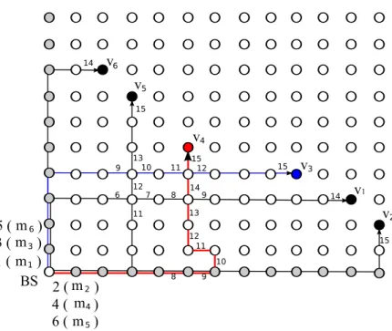
Example 3 Consider the following example (see Figure 6). We have 6 messages mi (1 ≤ i ≤ 6) with
destinations at distanced for m1andm2,d − 1 for m3andd − 4 for m4, m5, m6. HereLB = d + 1,
achieved for m2, m3 and m6. In the Figure 6, d = 14, v1 = (11, 3), v2 = (12, 2), v3 = (9, 4),
v4 = (5, 5), v5 = (3, 7) and v6 = (2, 8) and LB = 15. If we apply OneApprox[dI = 0, last =
V ](M) we get the sequence (m1, m3, m2, m5, m4, m6) with a makespan 16 attained for s3= m2. If we
applyOneApprox[dI = 0, last = H](M) we get the sequence (m1, m2, m4, m3, m6, m5) also with a
makespan16 attained for s4 = m3. Consider any algorithm where the messages are sent via shortest
directed paths. If the makespan is LB thenm1andm2should be sent in the first two steps and to avoid
interferences the source should sendm1 via(0, 1) and m2via(1, 0). m3should be sent at step 3. If
m2was sent at step1 and so m1at step2, then m3should be sent at step3 via (1, 0) and will interfere
withm1. Therefore, the only possibility is to sendm1at step1 via (0, 1), m2at step2 via (1, 0) and m3
at step3 via (0, 1). But then at step 4, we cannot send any of m4, m5, m6without interference. So the
source does no sending at step4, but the last sent message will be sent at step 7 and the makespan will be d + 2 = LB + 1. However there exists a tricky schedule with makespan LB, but not with shortest directed paths routing. We sentm1vertically,m2horizontally,m3vertically butm4with a detour to introduce a
delay of2. More precisely, if v4= (x4, y4), we send m4horizontally till(x4+ 1, 0), then to (x4+ 1, 1)
and(x4, 1) (the detour) and then vertically till (x4, y4). Finally we send m6vertically at step5 and m5
horizontally at step6. m4has been delayed by two but the message arrives at timeLB and there is no
interference between the messages.
In view of this example it seems difficult to characterize what are the instances for which the makespan is LB and those for which the instance is LB + 1. The complexity of determining the value of the minimum makespan is also open. Perhaps the problem would be simpler if we restrict ourselves to use only shortest directed path routings (or basic schemes). We will use this idea of detour in Section 5 to get efficient algorithms for dI ∈ {1, 2}.
4
Case d
I= 0; general grid, and BS in the corner
We will see in this section that, by generalizing the notion of basic scheme, Algorithm T woApprox[dI =
0, last = D](M) also achieves a makespan at most LB + 2 in the case of a general grid, that is when the destinations of the messages can be on one or both axes and with BS in the corner. First we have to extend the notions of horizontal sendings for a destination node on Y-axis and vertical sendings for a destination node on the X-axis. However the proof of the basic lemmas is more complicated as Lemma 3 is not fully valid in this case.
We will say that a message is sent “horizontally to reach the Y axis”, denoted by HY-sending, if the
destination of m is on the Y axis, i.e., dest(m) = (0, y), and the message is sent first horizontally from BS to (1,0) then it follows the vertical directed path from (1, 0) till (1, y) and finally the horizontal arc ((1, y), (0, y)). Similarly a message is sent “vertically to reach the X axis”, denoted by VX-sending, if
the destination of m is on the X axis, i.e., dest(m) = (x, 0), and the message is sent first vertically from BS to (0,1) then it follows the horizontal directed path from (0, 1) till (x, 1) and finally the vertical arc ((x, 1), (x, 0)).
Notations. Definition 1 of basic scheme in Section 3.1 is extended by allowing HY (resp., VX)-sendings
as horizontal (resp., vertical) sendings. For emphasis, we call it modified basic scheme. Similarly we will use the notation of Section 3.1 (m, m0) ∈ HV (resp., (m, m0) /∈ HV ) when the message m is sent first
horizontally including HY-sending and the message m0 is sent at the step just after vertically including
VX-sending , and if they do not interfere (resp., if they interfere). We define similarly (m, m0) ∈ V H
(resp., (m, m0) /∈ V H).
Note that we cannot have an HY-sending followed by a VX-sending (or a VX-sending followed by an
HY-sending) as there will be interference in (1, 1).
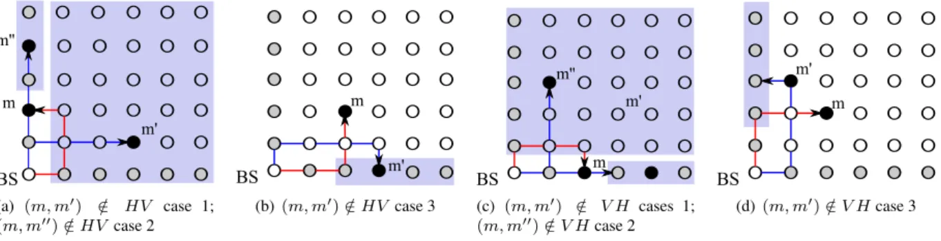
BS m' m m'' (a) (m, m0) ∈ HV case 1;/ (m, m00) /∈ HV case 2 BS m' m (b) (m, m0) /∈ HV case 3 BS m' m m'' (c) (m, m0) ∈ V H cases 1;/ (m, m00) /∈ V H case 2 BS m' m (d) (m, m0) /∈ V H case 3
Figure 7: Cases of interferences with destinations on the axis
Fact 4 Let dest(m) = (x, y) and dest(m0) = (x0, y0) and suppose at least one of them is on an axis. Then
• (m, m0) /∈ HV if and only if we are in one of the following cases 4.1: x = 0 and x0 > 0
4.2: x = 0, x0= 0 and y0 > y 4.3: x > 0, y0 = 0, x ≤ x0andy ≥ 2 or equivalently
4.4: y = 0
4.5: x = 0, x0 = 0 and y0≤ y 4.6: x > 0, y > 0, x0 = 0
4.7: x > 0, y > 0, y0= 0, and either y = 1 or x0< x
Proof. First suppose dest(m) is on one of the axis. If, y = 0 there is no interference (4.4). If x = 0 and y0> y message m arrives at its destination (0, y) at step y + 2, but message m0leaves (0, y) at step y + 2 and so they interfere (4.2 and 4.1 with y0> y). If x = 0 and y0≤ y, either x0 = 0 and the directed
paths followed by the messages do not cross (4.5), or x0 > 0, but then message m leaves (1, y0) at step y0+ 2, while message m0arrives at (1, y0) at step y0+ 2 and so they interfere (4.1 with y0≤ y).
Suppose now that dest(m) is not on one of the axis, that is x > 0 and y > 0. If x0 = 0, the directed paths followed by the messages do not cross (4.6). If y0= 0, then either x0 < x and the messages do not
interfere (4.7) or x0 ≥ x, and the directed paths cross at (x, 1) and there either y = 1 and the messages do not interfere (4.7) or y ≥ 2 , but then message m leaves (x, 1) at step x + 2, while message m0arrives at (x, 1) at step x + 2 and so they interfere (4.3).
By exchanging x and y and also H and V we get:
Fact 5 Let dest(m) = (x, y) and dest(m0) = (x0, y0) and suppose at least one of them is on an axis. Then
• (m, m0) /∈ V H if and only if we are in one of the following cases 5.1: y = 0 and y0 > 0
5.2: y = 0, y0= 0 and x0> x 5.3: y > 0, x0= 0, y ≤ y0andx ≥ 2 or equivalently
• (m, m0) ∈ V H if and only if we are in one of the following cases 5.4: x = 0 5.5: y = 0, y0= 0 and x0≤ x 5.6: x > 0, y > 0, y0= 0 5.7: x > 0, y > 0, x0 = 0, and either x = 1 or y0< y Lemma 5 • If(m, m0) /∈ HV , then (m, m0) ∈ V H. • If(m, m0) /∈ V H, then (m, m0) ∈ HV .
Proof. If none of the destinations of m and m0are on the axis, the result holds by Lemma 1. If at least one destination is on an axis, suppose that (m, m0) /∈ HV . If conditions of Fact 4.1 or 4.2 are satisfied, then x = 0 but then by Fact 5.4 (m, m0) ∈ V H. If condition of Fact 4.3 is satisfied , so x > 0, y0 = 0 and y ≥ 2 which implies by Fact 5.6 that (m, m0) ∈ V H. The second claim is obtained similarly.
Similarly we get the generalization of Lemma 2. Lemma 6 • If(m, m0) /∈ HV , then (m0, m) ∈ HV .
• If(m, m0) /∈ V H, then (m0, m) ∈ V H.
Lemma 7 Let dest(m) = (x, y), dest(m0) = (x0, y0) and dest(m00) = (x00, y00)
• If(m, m0) ∈ HV and (m0, m00) /∈ V H, then (m, m00) ∈ HV , except if y0 = 0 (V
X-sending is
used form0), andy ≥ max(2, y00+ 1), and 0 < x0 < x ≤ x00, in which case(m, m00) /∈ HV . • If(m, m0) ∈ V H and (m0, m00) /∈ HV , then (m, m00) ∈ V H,
except ifx0= 0 (HY-sending is used form0), andx ≥ max(2, x00+ 1), and 0 < y0 < y ≤ y00, in
which case(m, m00) /∈ V H.
Proof. Let us prove the first claim. If none of the destinations of m, m0, m00 are on an axis the result holds by Lemma 3. If y = 0, then (m, m00) ∈ HV by Fact 4.4. By Fact 5, (m0, m00) /∈ V H implies x0 > 0. If x = 0, then by Fact 4.5, (m, m0) ∈ HV implies x0 = 0 a contradiction with the preceding assertion. Therefore x > 0 and dest(m) is not on an axis. Now, if x00= 0 by Fact 4.6 (m, m00) ∈ HV . If y0 > 0, then (m0, m00) /∈ V H implies x00 = 0 by Fact 5.3, where we already know that by Fact 4.6
(m, m00) ∈ HV . So y0 = 0, x > 0, y > 0 and by Fact 4.7 (m, m0) ∈ HV implies that either y = 1 or
x0 < x.
If y00 = 0, by Fact 4.3, (m, m00) /∈ HV if and only if y ≥ 2 and x ≤ x00. If y00 > 0, none of the
destinations of m and m00are on the axis and so by Fact 2, (m, m00) /∈ HV , if and only if x00≥ x and
y00 < y. So again y ≥ 2 and x ≤ x00. In summary (m, m00) /∈ HV , if and only if y ≥ 2 and when y00> 0, y > y00and 0 < x0 < x ≤ x00
The second claim is obtained similarly.
We give the following useful corollary for the proof of the next theorem. Corollary 1 If d(m0) ≥ d(m00) then:
• If(m, m0) ∈ HV and (m0, m00) /∈ V H, then (m, m00) ∈ HV .
• If(m, m0) ∈ V H and (m0, m00) /∈ HV , then (m, m00) ∈ V H.
Proof. Indeed by the preceding lemma if (m, m00) /∈ HV , then y0 = 0, x0< x00and so d(m0) < d(m00). We now show that Lemma 4 is still valid in general grid.
Lemma 8 • If(m, m0) /∈ HV and (m, m00) /∈ V H, then (m0, m00) ∈ HV .
• If(m, m0) /∈ V H and (m, m00) /∈ HV , then (m0, m00) ∈ V H.
Proof. If none of the destinations of m, m0, m00are on an axis the result holds by Lemma 4. Suppose first
dest(m00) is on an axis; by Fact 5 (m, m00) /∈ V H implies x > 0. If furthermore dest(m) or dest(m0) are
on an axis, by Fact 4.3 (m, m0) /∈ HV implies y0= 0 and so by Fact 4.4 (m0, m00) ∈ HV . Otherwise if none of dest(m) and dest(m0) are on an axis, y > 0 and by Fact 5.3 (m, m00) /∈ V H implies x00= 0, and
with x0> 0 and y0> 0 Fact 4.6 implies (m0, m00) ∈ HV .
If dest(m00) is not on an axis, then one of dest(m) and dest(m0) is on an axis and (m, m0) /∈ HV implies y > 0. We cannot have x = 0 otherwise it contradicts (m, m00) /∈ V H. If x > 0, then by Fact 4.3 (m, m0) /∈ HV implies y0= 0, but then Fact 4.4 implies (m0, m00) ∈ HV . The second claim is obtained
similarly.
Theorem 6 Let dI = 0, and BS be in the corner of the general grid. Given an ordered (by
non-increasing distance) sequence of messages M = (m1, m2, · · · , mM) and a direction D, Algorithm
T woApprox[dI = 0, last = D](M) computes in linear-time an ordering S of the messages satisfying
following properties


](https://thumb-eu.123doks.com/thumbv2/123doknet/12961857.376870/15.892.161.803.176.490/figure-algorithm-t-woapprox-i-last-v-m.webp)
 and OneApprox[d I = 0, last = V ](M)](https://thumb-eu.123doks.com/thumbv2/123doknet/12961857.376870/16.892.74.741.293.514/figure-examples-algorithms-t-woapprox-i-d-oneapprox.webp)
(case when the last message is sent vertically)](https://thumb-eu.123doks.com/thumbv2/123doknet/12961857.376870/18.892.109.747.256.635/figure-algorithm-oneapprox-i-case-message-sent-vertically.webp)