HAL Id: cea-01342149
https://hal-cea.archives-ouvertes.fr/cea-01342149
Submitted on 5 Jul 2016
HAL is a multi-disciplinary open access
archive for the deposit and dissemination of
sci-entific research documents, whether they are
pub-lished or not. The documents may come from
teaching and research institutions in France or
abroad, or from public or private research centers.
L’archive ouverte pluridisciplinaire HAL, est
destinée au dépôt et à la diffusion de documents
scientifiques de niveau recherche, publiés ou non,
émanant des établissements d’enseignement et de
recherche français ou étrangers, des laboratoires
publics ou privés.
model with long range interactions
Li Huang, Thomas Ayral, Silke Biermann, Philipp Werner
To cite this version:
Li Huang, Thomas Ayral, Silke Biermann, Philipp Werner. Extended dynamical mean-field study
of the Hubbard model with long range interactions. Physical Review B: Condensed Matter and
Materials Physics (1998-2015), American Physical Society, 2014, 90 (19), pp.5114.
�10.1103/Phys-RevB.90.195114�. �cea-01342149�
arXiv:1404.7047v2 [cond-mat.str-el] 17 Oct 2014
interactions
Li Huang,1 Thomas Ayral,2, 3 Silke Biermann,2 and Philipp Werner1 1
Department of Physics, University of Fribourg, 1700 Fribourg, Switzerland 2
Centre de Physique Th´eorique, Ecole Polytechnique, CNRS-UMR7644, 91128 Palaiseau, France 3
Institut de Physique Th´eorique (IPhT), CEA, CNRS, URA 2306, 91191 Gif-sur-Yvette, France (Dated: October 20, 2014)
Using extended dynamical mean-field theory and its combination with the GW approximation, we compute the phase diagrams and local spectral functions of the single-band extended Hubbard model on the square and simple cubic lattices, considering long range interactions up to the third nearest neighbors. The longer range interactions shift the boundaries between the metallic, charge-ordered insulating and Mott insulating phases, and lead to characteristic changes in the screening modes and local spectral functions. Momentum-dependent self-energy contributions enhance the correlation effects and thus compete with the additional screening effect from longer range Coulomb interactions. Our results suggest that the influence of longer range intersite interactions is significant, and that these effects deserve attention in realistic studies of correlated materials.
PACS numbers: 71.15.-m, 71.10.Fd, 71.30.+h
I. INTRODUCTION
In condensed matter physics, electron-electron corre-lations give rise to many intriguing phenomena rang-ing from simple energy band renormalization to complex phase diagrams with charge-, spin-, or orbital ordering.1
The essential physics is the competition between elec-tron localization and itinerancy. The Hubbard model is one of the simplest models which captures this compe-tition, and it is therefore often used to investigate cor-relation effects in lattice systems.2,3 For instance, it is
generally believed that the two-dimensional single-band Hubbard model with static onsite Coulomb interaction U can be used to explain some underlying physics of cuprate high-temperature superconductors.4One widely
accepted assumption in these studies is that the electron-electron interaction is local, i.e., that long range inter-site interactions are fully screened or may be ignored. When additional intersite Coulomb interactions are con-sidered, the model becomes an extended Hubbard model, which can be used for example to explore charge-ordering and Wigner-Mott transitions.5This model also describes
the screening of local interactions by the nonlocal in-teractions. Both the charge-ordering transition and the screening effect in the extended Hubbard model have been investigated in numerous theoretical studies.6–15
The physical properties of the Hubbard model have been studied extensively using the dynamical mean-field theory (DMFT).2,3 This approximate scheme describes
the generic behavior of high-dimensional lattice systems. In particular, at half-filling and low temperature, the DMFT solution for the hypercubic lattice will be an antiferromagnetically ordered insulator, whose charac-ter changes from a Slacharac-ter-type antiferromagnet at weak interactions, to a Heisenberg-type antiferromagnet with local moments at large interaction. If the calculations are restricted to the paramagnetic phase, the DMFT method predicts a transition from a Fermi-liquid metal
to a Mott insulator at a temperature-dependent criti-cal value of the onsite interaction U (comparable to the bandwidth). This paramagnetic Mott transition can be considered as the generic physical situation at sufficiently high temperatures, or in the magnetically frustrated case. The extended Hubbard model with strong non-local in-teractions (parametrized by V ) exhibits a transition to a charge-ordered state characterized by a freezing of charge carriers and a spatial modulation of the charge density.5 To describe this transition one may resort to
the extended dynamical mean-field theory (EDMFT) framework.7,16–22 The basic idea of EDMFT was
origi-nally developed in studies of heavy-fermion systems and spin glasses with non-local Coulomb interactions.16,17
The physical effects induced by the nonlocal interac-tion V , including a frequency dependence of the effec-tive local interaction and a sizable reduction of the static value of U , are well captured by the EDMFT scheme. Since EDMFT takes into account the spatially nonlocal interactions beyond the Hartree level, it is a sophisti-cated numerical tool for studying the extended Hubbard model. However, EDMFT is still based on a local ap-proximation, i.e., it assumes a k-independent self-energy function and polarization function. To further incorpo-rate spatially nonlocal contributions into these functions, one can combine the EDMFT approach with the GW approximation.6,7,14,15,22
While the EDMFT and GW + EDMFT schemes have been developed more than ten years ago, there has been a recent revival in interest in these approaches, due to methodological improvements which enable an effi-cient and accurate solution of the self-consistency equa-tions. In the previous studies, phase diagrams in the space of onsite interaction U and the nearest neighbor interaction V , fully screened and retarded interactions, and local spectral functions have been calculated for the extended Hubbard model on square and simple cu-bic lattices.7,14,15,20,22 It has been found that the
criti-cal charge-ordering lines Vc(U ) between the Mott
insu-lator phase and the charge-ordered insuinsu-lator phase ob-tained by the EDMFT and GW + EDMFT approaches are substantially steeper than the naive mean-field esti-mate Vc = U/z, where z is the number of the nearest
neighbors.15This may point to an overestimation of the
local interactions in the EDMFT and GW + EDMFT schemes or a non-trivial screening effect. Further issues left open in previous work concern the physical interpre-tation of the dominant screening processes, and their de-pendence on the parameters of the model. In Ref.23, it was proposed that the effective local interaction incorpo-rating screening by neighboring lattice sites can be well approximated by simple estimates in terms of onsite and intersite interactions. The recent GW + EDMFT study of Ref.15was consistent with this simple picture in the correlated metallic case in two dimensions with nearest neighbor interactions. However, the usefulness and accu-racy of these estimates in the higher dimensional case or with longer range interactions remains an open question. The early studies of the three-dimensional extended Hubbard model7,22 used a modified Hirsch-Fye
algo-rithm to solve the effective impurity problem and could not reach low temperatures. In these calculations, the fermionic part of the impurity model was handled by a standard Hirsch-Fye algorithm,2,3 while the
statisti-cal weight due to the continuous bosonic fields was ob-tained directly by computing the corresponding Boltz-mann factor.24This algorithm is not as efficient and
ac-curate as the recently developed continuous time quan-tum Monte Carlo (CT-QMC) solver25–28which can treat
systems with a frequency-dependent retarded interaction without any approximations. Thus, it is worthwhile to reinvestigate the model using the EDMFT and GW + EDMFT approaches in combination with the state-of-the-art CT-QMC quantum impurity solver. This was done in Refs. 14 and 15 for the two-dimensional model with local and nearest neighbor interactions. Here, we extend the investigation to the three-dimensional model and to interactions of longer range. Indeed, recent constrained random phase approximation calculations29
and a recent GW + EDMFT study30 of adatom
sys-tems Si(111):X, with X = Sn, Si, C, Pb, suggests that taking into account substantially longer range interac-tions is mandatory to understand experimentally ob-served trends from Mott physics toward charge-ordering physics along this series. In particular, it was shown that long-range interactions (for the surface systems, the full Coulomb tail was considered) can decrease the effective local interaction by up to a factor of two. Similar con-clusions were drawn in Ref.23for other two-dimensional systems like graphene, silicene and benzene. Other stud-ies suggest that the superconducting Tc is generally
sup-pressed in some pairing channels as the strength of longer range interactions increases.13It thus appears that longer range intersite interactions beyond the nearest neighbors may be important, at least for low dimensional systems. So, it is worth investigating in a simple model context
how longer range intersite interactions modify the phase diagrams and various local and nonlocal observables.
The purpose of this paper is to gain qualitative and quantitative insights into the role of screening from non-local Coulomb interactions. For this, we study the ex-tended Hubbard model on the square (2D) and simple cubic (3D) lattices using a modern EDMFT and GW + EDMFT implementation with a numerically exact CT-QMC impurity solver. The calculations are restricted to repulsive interactions U > 0 and V > 0, and to the paramagnetic phase, so that we can investigate the par-ticularly interesting screening effects in the correlated metal, close to the Mott or charge ordered insulator phase boundaries. In particular, we extract the domi-nant screening modes and analyze the effects of longer range intersite interactions on local, but energy depen-dent observables, such as spectral functions. At first, we will perform self-consistent EDMFT calculations to map out the entire U −V phase diagram, and then compare to GW + EDMFT results at some representative points to gain insights into the effects of nonlocal self-energy and polarization contributions.
The rest of this paper is organized as follows. SectionII
defines the extended Hubbard model used in this study. The flowcharts for the EDMFT and GW + EDMFT methods and the computational details are also briefly summarized in this section. SectionIII Ashows the re-sults obtained using the EDMFT approach. The phase diagrams, fully screened and retarded interactions in-duced by the V term, and local spectral functions are presented and discussed in detail. Especially, doping-dependent phase diagrams and related bosonic spectral functions are also presented in this section. Some rep-resentative results obtained with the GW + EDMFT approach are discussed in Sec. III B. A brief summary and outlook are given in Sec.IV. Appendix Adescribes the long range intersite interactions considered in the 2D and 3D extended Hubbard models, while Appendix B
details the maximum entropy based analytical continu-ation method used to extract the spectral functions for the frequency-dependent fully screened and retarded in-teractions.
II. MODEL AND METHODS
A. Extended Hubbard model
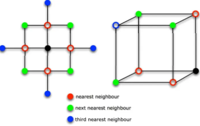
In the present study, we consider the single-band ex-tended Hubbard models on a two-dimensional square lattice and a three-dimensional simple cubic lattice, re-spectively (see schematic picture in Fig.1). The grand-canonical Hamiltonian can be written as
H = − X (i,j),σ tij(c†iσcjσ+ H.c) − µ X i ni + UX i ni↑ni↓+ X (i,j) Vijninj, (1)
nearest neighbour next nearest neighbour third nearest neighbour
FIG. 1. (Color online) Schematic picture of the one-band half-filled extended Hubbard model in the charge-ordered state for the square lattice (left) and simple cubic lattice (right). The full dots represent doubly occupied sites and the open dots empty sites. The red, green, and purple dots denote the NN, NNN, and 3NN sites of the black dot, respectively.
where i and j are site indices and (i, j) denotes a pair of sites i and j. ciσand c†iσare the annihilation and creation
operators of an electron of spin σ at the lattice site i. niσ
is the orbital occupation operator, and ni = ni↑+ ni↓.
tij is the hopping matrix element between two different
sites, µ the chemical potential, U the onsite interaction, and Vij the intersite interaction between sites i and j.
When i = j, both tij and Vij must be zero. Only the
hopping between the nearest neighbor (NN) sites is al-lowed in this study, namely, tij = thiji= t > 0. However,
for the nonlocal repulsive interactions Vijwe also consider
the next nearest neighbor (NNN) and the third nearest neighbor (3NN) sites. Our definitions for the NN, NNN and 3NN sites are shown in Fig. 1. We further assume that Vij can be calculated by scaling V with a/|~ri− ~rj|,
in other words, with the inverse distance in units of the NN distance a. In this sense, V is not only the NN in-teraction, but also the parameter which determines the strength of all the long range Coulomb interactions. The detailed formulas of the Fourier-transformed tij and Vij
are given in AppendixA.
B. EDMFT and GW + EDMFT
We solve the single-band extended Hubbard model [see Eq. (1)] with fully self-consistent EDMFT and GW + EDMFT calculations. The EDMFT approach with the “U V decoupling” scheme15 formally treats the local
in-teractions and nonlocal intersite inin-teractions on the same footing. It can be used to describe the Mott transi-tion and charge-ordering transitransi-tion in the extended Hub-bard model.16,17,20,21 The idea of the combined GW + EDMFT6 scheme is the following: One takes the local
part of the self-energy (or polarization) from the EDMFT calculation and adds to it the nonlocal component of the
GW self-energy (or polarization). Thus, a momentum dependence is introduced into the self-energy (or polar-ization), and the scheme captures the interplay of screen-ing and nonlocal correlations at least to some extent. While the accuracy of the scheme has not been system-atically tested, self-consistent GW + EDMFT calcula-tions can be obtained in the whole interaction range from the weakly correlated region to the atomic limit. A de-tailed derivation of the GW + EDMFT formulation for extended Hubbard model can be found in Ref.15.
The typical GW + EDMFT self-consistency loop in-volves the following steps.7,15 One starts with an initial
guess for the k-dependent fermionic self-energy Σ(k, iωn)
and the bosonic self-energy (or polarization) Π(k, iνn),
with Matsubara frequencies ωn = (2n + 1)π/β and
νn = 2nπ/β for integer n. The initial Σ(k, iωn) and
Π(k, iνn) can be obtained from previously calculated
re-sults, or chosen to be zero. Then one calculates the lattice Green’s function G(k, iωn) and fully screened interaction
W (k, iνn) using the lattice Dyson equations
G(k, iωn) = 1 iωn+ µ − ǫk− Σ(k, iωn) , (2) and W (k, iνn) = 1 v−1k − Π(k, iνn) . (3)
Here, ǫk is the band dispersion and vk is the bare
in-teraction in reciprocal space (see Appendix A for more details). Then the local counterparts of G, W , Σ and Π are calculated by averaging over the whole Brillouin zone, for instance (Nk is the number of k-points),
G(iωn) = 1 Nk X k G(k, iωn). (4)
Next, the local bath Green’s function G(iωn) and
fre-quency dependent retarded interaction U(iνn) are
calcu-lated through the impurity Dyson equations, namely, G−1(iωn) = G−1(iω) + Σ(iωn), (5)
and
U−1(iνn) = W−1(iνn) + Π(iνn). (6)
Then the quantum impurity model defined by G(iωn) and
U(iνn) is solved numerically. The impurity solver directly
yields the new G(iωn). On the other hand, the
calcula-tion of the new W (iνn) involves as an intermediate step,
the calculation of the connected charge-charge correlation function χ(τ ) = hT ¯n(τ)¯n(0)i with ¯n = n−hni. From the Fourier-transformed χ(iνn) and U(iνn), we finally obtain
the new W (iνn) via
W (iνn) = U(iνn) − U(iνn)χ(iνn)U(iνn). (7)
Using these G(iωn) and W (iνn) as inputs, the new local
by using Eqs. (5) and (6) again. Within the GW approx-imation, one evaluates the momentum-dependent GW self-energy and polarization functions as ΣGW = −GW
and ΠGW = 2GG.6 Here the factor 2 comes from the
contribution of the spin degree of freedom. Finally, one has to separate the local and nonlocal parts of these GW self-energies and polarizations,
ΣGW loc (iωn) = 1 Nk X k ΣGW(k, iω n), (8) ΠGWloc (iνn) = 1 Nk X k ΠGW(k, iνn), (9)
ΣGWnonloc(k, iωn) = ΣGW(k, iωn) − ΣGWloc (iωn), (10)
ΠGWnonloc(k, iνn) = ΠGW(k, iνn) − ΠGWloc (iνn), (11)
and then combine the nonlocal parts with the local con-tributions obtained from the impurity calculations, i.e., Σ(k, iωn) = ΣGWnonloc(k, iωn) + Σ(iωn), (12)
and
Π(k, iνn) = ΠGWnonloc(k, iνn) + Π(iνn). (13)
The new self-energy and polarization functions, Σ(k, iωn)
and Π(k, iνn), serve as the starting point of the next
it-eration. This completes the self-consistent loop.
The EDMFT self-consistency loop can be viewed as a simplification of the full GW + EDMFT iteration, where one ignores the calculations of the GW self-energies ΣGW(k, iω
n) and polarizations ΠGW(k, iνn), and adopts
the following local approximations
Σ(k, iωn) = Σ(iωn), (14)
and
Π(k, iνn) = Π(iνn). (15)
In the following calculations, we consider half-filled single-band extended Hubbard models on the square lat-tice and simple cubic latlat-tice (some results for the 2D model away from half-filling can be found in Sec.III A). The k-sums are discretized in the irreducible Brillouin zone on 81 × 81 and 19 × 19 × 19 grid points, respectively. We used the hybridization expansion quantum impurity solver to solve the effective impurity problems.27,28 The
imaginary time Green’s function G(τ ) and charge-charge correlation function χ(τ ) are measured on N = 1024 equally spaced time points. We used 4t as the unit of energy and performed calculations at inverse tempera-ture β = 100, restricting our study to the paramagnetic phase. Up to 40 EDMFT and GW + EDMFT itera-tions are required to reach convergence when the system is close to the Mott or charge-ordering transition.
C. Analytical continuation
Since the self-consistency loop is implemented fully on the imaginary time/frequency axis, we have to analyti-cally continue the converged G(τ ), U(iν), and W (iν) to obtain meaningful information about single particle ex-citations and screening modes.
The frequency dependence of the retarded interaction U(iν) affects the single particle spectral function A(ω), and in particular induces satellites at energies which are determined by the dominant screening frequencies.27,31,32
However, the classical maximum entropy method,33
which is commonly used to perform analytical contin-uations of G(τ ), tends to smooth out these high-energy features. To overcome this obstacle, we adopted the al-gorithm proposed by Casula et al.31 and proceed as
fol-lows: From the spectral function ImU(ν) we calculate the bosonic function B(τ ) = exp[K(0) − K(τ)], (16) where34 K(τ ) = Z ∞ 0 dνImU(ν) ν2 cosh[ν(β/2 − τ)] sinh(νβ/2) , (17) and the corresponding spectral function AB(ν). We then
define the auxiliary fermionic Green’s function Gaux(τ ) =
G(τ )/B(τ ), which later is analytically continued us-ing the conventional maximum entropy method to yield Aaux(ω). Finally, the spectral function for G(τ ) is
ob-tained from the convolution A(ω) =
Z
dǫAB(ǫ)Aaux(ω − ǫ)(1 + e
−βω)
(1 + eβ(ǫ−ω))(1 − e−βǫ) . (18)
This procedure requires an accurate estimate of the spectral function ImU(ν). In previous studies, the Pad´e approximation was used.15 However, we found that the
Pad´e results are very sensitive to the data quality of U(iν). Small fluctuations in U(iν), which are almost un-avoidable [see Eq. (6)], can lead to drastic modifications in the Pad´e estimation of ImU(ν). Thus, a robust proce-dure with respect to the typical level of numerical noise is crucial. The maximum entropy method is superior in this respect, and we have adapted it to the problem of analytically continuing the retarded interaction U(iν) and fully screened interaction W (iν). The details of this procedure are explained in AppendixB.
III. RESULTS AND DISCUSSION
A. EDMFT results
In this subsection, we present self-consistent EDMFT results for the paramagnetic, half-filled single-band U -V Hubbard model on the square lattice and simple cubic lattice. All results are for inverse temperature β = 100.
1. U -V phase diagrams
Figure2shows the phase diagrams in the space of the parameters U and V . In this figure, the left panel shows the result for the square lattice, and the right panel corre-sponds to the simple cubic lattice. Both phase diagrams exhibit three phases: a metallic Fermi-liquid (FL) phase in which the kinetic energy dominates the interactions, the Mott insulating (MI) phase with one particle per site, where U is dominant, and the charge-ordered (CO) insu-lator with a charge density wave (CDW) when V prevails. The insets plot the phase diagrams with axes rescaled by the bandwidth (8t for the square lattice and 12t for the simple cubic lattice), to emphasize the similarities and differences between the 2D and 3D cases.
The paramagnetic phase diagram for the extended Hubbard model with the NN interactions on the square lattice is consistent with the result by Ayral et al.15
The paramagnetic phase diagram for the simple cubic lattice with the NN interactions has been calculated in the pioneering paper by Sun et al.7 Their calculations
however were performed at a much higher temperature (β = 5), above the end-point of the FL-MI transition. Also, the quantum impurity solver used in that study was a modified Hirsch-Fye algorithm with Bose factor approximation,24 which is not as accurate as the
nu-merically exact CT-QMC algorithm.27 Taking into
ac-count these differences, the phase diagram presented in Fig.2(b) appears to be qualitatively consistent with the previous result by Sun et al.7 When the temperature is
increased, the Vc(U ) line shifts upwards, and the Uc(V )
line is shifted to the left. In contrast to the paramag-netic MI, the CO insulator does not have a large entropy of ln 2 per site (the phase boundary is determined from the divergence in the charge susceptibility, see subsection
III A 2for further details).
In the previous calculations, only the NN intersite in-teractions have been included. In the present work, we also consider the effects of longer range interactions, more specifically the NNN and 3NN intersite interactions, as depicted in Fig.1. In a future study, it would be inter-esting to consider the effect of an infinite range Coulomb 1/r-type tail. A proper treatment of it requires an Ewald lattice summation, as is shown by Hansmann et al.30
The modifications in the phase diagram for the square lattice are shown in Fig. 2(a). When U is small, the Vc(U ) lines is shifted upward if the NNN and 3NN
inter-actions are added, which means that these longer range intersite interactions destabilize the CO state. This is not surprising, since the left panel of Fig. 1 shows that both the NN and 3NN interactions act between sites of the same sub-lattice, and hence penalize the CDW. In the strongly correlated region, the Vc(U ) line is shifted
downward, which means that the MI state is suppressed by longer range intersite interactions, which can be in-terpreted as the result of the enhanced screening of the onsite interaction. For the same reason, the Uc(V ) line
is slightly shifted to the right. Finally, if only the NN
in-tersite interaction is considered, the Vc(U ) line “jumps”
in the region where the Vc(U ) and Uc(V ) lines intersect,
and this jump is accompanied by a change of the slope. If longer range interactions are included, the metallic phase extends to larger values of U , so that the transition be-tween MI and CO phases is no longer a direct one, at least for 2.5 . U . 3.0. As a result of this interme-diate metallic phase, the jump in the Vc(U ) line
disap-pears. We note that the shape of the metallic phase with longer range interactions is qualitatively similar to the FL phase in the single-band Holstein-Hubbard model with large phonon frequency.27One difference is that the
phase diagram for the Holstein-Hubbard model does not have a sudden slope change in the phase boundary to the CO phase in the vicinity of the Mott transition. This suggests that the slope change in the extended Hubbard model originates from changes in the screening processes near Uc. We will investigate this issue in more detail in
subsectionIII A 3.
Next, let’s turn to the simple cubic lattice case [see Fig.2(b)]. Here, for small U , the Vc(U ) phase boundary
is shifted upward when the NNN interaction is added, just as in the 2D case, but the 3NN interaction has the opposite effect. Therefore, the shift is not monotonous any more. This can be understood by looking at the right hand panel of Fig.1. While the NNN interactions act between sites on the same sub-lattice, and hence frus-trate the CDW, the 3NN interactions act between sites on different sub-lattices, and thus favor the CO phase. Another difference to the 2D case is that the metallic region between the MI and CO phases is larger, so that there is no obvious “kink” or sudden “jump” in the Vc(U )
line near the Mott transition. In fact, for the model with only the NN interactions, the slope change in the Vc(U )
line happens already quite a bit before the Mott transi-tion (Uc∼ 3.1) at V = 0.
2. Charge-ordering and Mott metal-insulator transitions
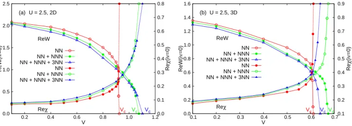
The phase transition from the FL and MI phases to the CO phase is signaled by a diverging charge susceptibility χ(iν = 0).7This divergence almost coincides with a sign
change in the fully screened interaction ReW (iν = 0) [see Eq. (7)]. When V increases, ReW (iν = 0) gets smaller, and when it reaches zero, the cost for the for-mation of doublons vanishes.15 In Fig. 3, the real parts
of W (iν = 0) and χ(iν = 0) are plotted against V for U = 2.5, which is still in the metallic state for the square and simple cubic lattices. The phase boundary to the CO state has been located by approaching the phase transition from below Vc. Actually, before Reχ(iν = 0)
diverges or ReW (iν = 0) reaches zero, we already en-counter a numerical instability which prevents the con-vergence of the EDMFT self-consistency loop. Thus, we extrapolate the curves using (V − Vc)−1, as shown by the
dashed lines in Fig.3, to determine the critical Vc. While
0.0 0.5 1.0 1.5 2.0 2.5 3.0 3.5 4.0 4.5 1.0 1.5 2.0 2.5 3.0 3.5 4.0 V U (a) CO FL MI NN NN + NNN NN + NNN + 3NN 0.0 0.2 0.4 0.6 0.8 1.0 1.2 0.5 0.7 0.9 1.1 1.3 1.5 V/W U/W 0.0 0.5 1.0 1.5 2.0 2.5 3.0 3.5 1.0 1.5 2.0 2.5 3.0 3.5 4.0 V U (b) CO FL MI NN NN + NNN NN + NNN + 3NN 0.0 0.2 0.4 0.6 0.8 1.0 1.2 0.5 0.7 0.9 1.1 1.3 1.5 V/W U/W
FIG. 2. (Color online) The paramagnetic U -V phase diagrams for the single-band half-filled extended Hubbard model deter-mined by EDMFT calculations. (a) Phase diagram for the 2D square lattice. (b) Phase diagram for the 3D simple cubic lattice. Here CO denotes a charge-ordered insulating phase, FL the metallic state, and MI the Mott insulator. The dashed lines are extrapolated FL-MI phase boundaries. The insets in (a) and (b) show the phase diagrams with axes rescaled by the bandwidth.
0.0 0.5 1.0 1.5 2.0 2.5 0.2 0.4 0.6 0.8 1.0 1.20.0 0.1 0.2 0.3 0.4 0.5 0.6 0.7 0.8 ReW(i ν =0) Re χ (i ν =0) V Vc Vc Vc U = 2.5, 2D (a) Reχ ReW NN NN + NNN NN + NNN + 3NN NN NN + NNN NN + NNN + 3NN 0.0 0.2 0.4 0.6 0.8 1.0 1.2 1.4 1.6 0.1 0.2 0.3 0.4 0.5 0.6 0.7 0.1 0.2 0.3 0.4 0.5 0.6 0.7 0.8 0.9 ReW(i ν =0) Re χ (i ν =0) V Vc VcVc U = 2.5, 3D (b) Reχ ReW NN NN + NNN NN + NNN + 3NN NN NN + NNN NN + NNN + 3NN
FIG. 3. (Color online) ReW (iν = 0) (see left x-axis) and Reχ(iν = 0) (see right y-axis) as a function of V . U = 2.5. (a) Results for the square lattice. (b) Results for the simple cubic lattice. The dashed lines are used to determine Vc for the
charge-ordering transition.
trend is unambiguous: In the square lattice case, Vc
in-creases as we add longer range interactions, even though for V . 0.9, the trend is actually opposite (due to an increasing screening effect). For the simple cubic lattice, the screening effect leads to a reduction of ReW (iν = 0) with increasing range of the interaction for V . 0.6, but then the drop to zero occurs in a non-monotonic way, for reasons related to lattice geometry as discussed above. In the large-U region, close to the Mott transition, the Vc(U ) phase boundary shifts down with increasing range
of the interaction, both for the square and the simple cu-bic lattice. This indicates that the interaction induced changes in the screening function should play the domi-nant role there.
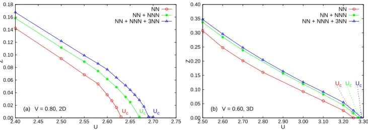
The phase boundary between metal and Mott insu-lator is signaled by a vanishing spectral weight at the
Fermi level. We increased the onsite interaction U step by step to approach the phase transition from the FL metallic side, so that our Uc values indicate the stability
region of the metallic phase (U < Uc). In our
calcula-tions, the Mott metal-insulator transition is determined by computing the quasiparticle weight Z2
Z = " 1 − ImΣ(iωω 0) 0 #−1 , (19)
where ω0 is the first Matsubara frequency ω0 = π/β.
Strictly speaking, this equation is only valid at zero tem-perature, but our temperature is low enough (β = 100) that it can be regarded as a good approximation. In Fig. 4, the calculated quasiparticle weights Z for the square and simple cubic lattices are plotted for selected
0.00 0.02 0.04 0.06 0.08 0.10 0.12 0.14 0.16 0.18 2.40 2.45 2.50 2.55 2.60 2.65 2.70 2.75 Z U Uc Uc Uc V = 0.80, 2D (a) NN NN + NNN NN + NNN + 3NN 0.00 0.05 0.10 0.15 0.20 0.25 0.30 0.35 0.40 2.50 2.60 2.70 2.80 2.90 3.00 3.10 3.20 3.30 Z U Uc Uc Uc V = 0.60, 3D (b) NN NN + NNN NN + NNN + 3NN
FIG. 4. (Color online) Quasiparticle weight Z as a function of U . (a) Results for the square lattice, V = 0.80. (b) Results for the simple cubic lattice, V = 0.60. When Z goes to zero, the Mott-Hubbard metal-insulator transition occurs. The corresponding U is Uc. In panel (b) the dashed lines are used to guide the eyes.
V parameters. This figure shows that longer range inter-site interactions lead to a larger Z and hence to a larger Uc. The reason is again a larger screening effect.
3. Screened and retarded interactions
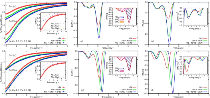
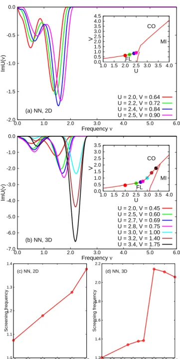
In the top panels of Fig. 5, we plot the real parts of W (iν) and U(iν), and the imaginary parts of W (ν) and U(ν) for the square lattice with selected U and V pa-rameters. The counterparts for the simple cubic lattice are shown in the bottom panels of Fig. 5. We concen-trate here on the FL region for both the 2D and 3D lat-tices. When ν → ∞, both the fully screened interactions ReW (iν) and partially screened interactions ReU(iν) [see Fig.5(a) and (b)] asymptotically approach the bare in-teraction U . As the frequency ν is lowered, ReW (iν) and ReU(iν) decrease monotonously. Longer range intersite interactions produce a stronger screening effect, and lead to lower values of the static interactions ReW (iν = 0) and ReU(iν = 0).
Let us take a closer look at the ImW (ν) and ImU(ν) spectra, which we have obtained from a modified max-imum entropy procedure33 (see Appendix B). To
ana-lyze the spectra, we fit ImW (ν) with multiple Gaussians. Each peak can be regarded as a screening mode (abbrevi-ated as SM), and the position of the peak corresponds to the screening frequency. Figures5(c) and (d) show that the ImW (ν) spectra feature two prominent SMs, whose screening frequencies differ by about a factor of two. The insets of Fig.5(a) and (b) show the contributions of these modes to the frequency dependence of ReW (iν). In the ImU(ν) spectra, one can also distinguish two humps, and the locations and weights of these screening modes are similar to the ImW (ν) counterparts. In both cases, the weight of the high-energy screening mode depends on the range of the intersite interaction. In the 3D case, the
high-energy mode also seems to shift in energy, as longer range interactions are included.
The physical interpretation of the two screening modes is somewhat subtle. As we will see in the following sec-tion, the spectral function in the metallic phase essen-tially exhibits a three-peak structure consisting of two Hubbard bands and a renormalized quasiparticle band. One can therefore distinguish screening processes stem-ming from transitions between the Hubbard bands, be-tween the quasiparticle peak and one of the Hubbard bands, and within the quasiparticle band.15It is natural
to associate the high-energy screening mode with inter-Hubbard band transitions and the low-energy mode with transitions from the quasiparticle peak to either Hubbard band. Consistent with this interpretation is the fact that the energy difference between the two modes is roughly a factor of two. Even the energy values associated with the two modes are in good agreement with the energy sepa-ration between the two Hubbard bands and between the quasiparticle and the Hubbard bands, respectively (see Fig.8below). One may however wonder why the bosonic spectra do not exhibit a low-energy mode related to transitions within the renormalized quasiparticle band. There is in fact no necessity for this to happen: even in the metallic phase, where Imχimp(ω) has a Drude-like
contribution παδ(ω) and hence, by the Kramers-Kronig relation, Reχimp = α/ω, the polarization Πimp does not
have a pole at ω = 0. Indeed, taking U = U for simplic-ity, we have Πimp= −χimp/(1 − Uχimp) = −α/(ω − αU).
As a result, the screened interaction does not have a pole at ω = 0 either: Wloc = Pqvq/(1 − vqΠimp) =
P
qvq(ω − αU)/(ω − α(U − vq)).
It is worth noting that the structures in the ImU(ν)/ν2
function, which are shown in the insets of Fig.5(e) and (f), determine the most relevant screening modes and the associated energies of satellites in the local spectral function A(ω).32 Therefore, despite the smaller weight,
1.2 1.4 1.6 1.8 2.0 2.2 2.4 0 1 2 3 4 5 6 ReW(i ν ) and ReU(i ν ) Frequency iν (a) U = 2.5, V = 0.8, 2D ReW(iν) ReU(iν) NN NN + NNN NN + NNN + 3NN 1.6 1.8 2.0 2.2 2.4 0 1 2 3 4 5 6 ReW(i ν ) Frequency iν NN, SM1 NN, SM2 NN, SM3 -6.0 -5.0 -4.0 -3.0 -2.0 -1.0 0.0 0 1 2 3 4 5 6 ImW( ν ) Frequency ν (c) NN NN + NNN NN + NNN + 3NN -4.0 -3.5 -3.0 -2.5 -2.0 -1.5 -1.0 -0.5 0.0 0 0.5 1 1.5 2 2.5 3 ImW( ν ) Frequency ν SM1 SM2 SM3 -2.0 -1.5 -1.0 -0.5 0.0 0 1 2 3 4 5 6 ImU( ν ) Frequency ν (e) NN NN + NNN NN + NNN + 3NN -1.0 -0.8 -0.6 -0.4 -0.2 0.0 0 0.5 1 1.5 2 2.5 3 ImU( ν )/ ν 2 Frequency ν 0.5 1.0 1.5 2.0 2.5 0 1 2 3 4 5 6 ReW(i ν ) and ReU(i ν ) Frequency iν (b) U = 2.5, V = 0.6, 3D ReW(iν) ReU(iν) NN NN + NNN NN + NNN + 3NN 0.5 1.0 1.5 2.0 2.5 0 1 2 3 4 5 6 ReW(i ν ) Frequency iν NN, SM1 NN, SM2 -10.0 -8.0 -6.0 -4.0 -2.0 0.0 0 1 2 3 4 5 6 ImW( ν ) Frequency ν (d) NN NN + NNN NN + NNN + 3NN -8.0 -7.0 -6.0 -5.0 -4.0 -3.0 -2.0 -1.0 0.0 0 0.5 1 1.5 2 2.5 3 ImW( ν ) Frequency ν SM1 SM2 -4.5 -4.0 -3.5 -3.0 -2.5 -2.0 -1.5 -1.0 -0.5 0.0 0 1 2 3 4 5 6 ImU( ν ) Frequency ν (f) NN NN + NNN NN + NNN + 3NN -3.5 -3.0 -2.5 -2.0 -1.5 -1.0 -0.5 0.0 0 0.5 1 1.5 2 2.5 3 ImU( ν )/ ν 2 Frequency ν
FIG. 5. (Color online) Real part of fully screened interactions ReW (iν) and partially screened interaction ReU(iν), imaginary part of real frequency fully screened interaction ImW (ν) and partially screened interactions ImU(ν) for the extended Hubbard model solved by EDMFT. (a), (c) and (e) Results for the square lattice, U = 2.5 and V = 0.8. (b), (d) and (e) Results for the simple cubic lattice, U = 2.5 and V = 0.6. In this figure, SM means screening mode. In the insets of (a) and (b) panels, the SM-resolved ReW (iν), together with full ReW (iν) are shown for the NN case. In (c) and (d) panels, the ImW (ν) for the NN case is approximated by Gaussian-type functions. The fitted results are shown in the insets. Each Gaussian peak denotes a SM. The insets in (e) and (f) panels show the ImU(ν)/ν2
functions. Here ImW (ν) and ImU(ν) are extracted using a modified maximum entropy method. See AppendixBfor more details.
Metallic state
Square lattice Simple cubic lattice
mode V U ReU(ν = 0) ReW (ν = 0) ν0 V U ReU(ν = 0) ReW (ν = 0) ν0
NN 0.80 2.50 2.14 (2.36) 1.51 (1.96) 1.61 (1.11) 0.60 2.50 1.68 (2.21) 0.73 (1.23) 1.44 (1.06) NN + NNN 0.80 2.50 2.03 (2.31) 1.34 (1.91) 1.77 (1.12) 0.60 2.50 1.65 (2.06) 0.62 (1.15) 1.96 (1.12) NN + NNN + 3NN 0.80 2.50 1.98 (2.28) 1.27 (1.86) 1.84 (1.10) 0.60 2.50 1.62 (2.03) 0.59 (1.14) 2.14 (1.16)
Mott insulating state
Square lattice Simple cubic lattice
mode V U ReU(ν = 0) ReW (ν = 0) ν0 V U ReU(ν = 0) ReW (ν = 0) ν0
NN 1.50 3.00 2.75 (2.82) 2.54 (2.61) 2.48 (1.75) 1.50 3.60 3.24 (3.33) 2.98 (3.08) 2.88 (2.16) NN + NNN 1.50 3.00 2.63 (2.75) 2.40 (2.55) 2.52 (1.66) 1.50 3.60 2.81 (3.04) 2.50 (2.79) 2.84 (2.00) NN + NNN + 3NN 1.50 3.00 2.56 (2.71) 2.34 (2.51) 2.54 (1.66) 1.50 3.60 2.56 (2.98) 2.27 (2.74) 2.87 (2.00) TABLE I. Summary of ReU(ν = 0), ReW (ν = 0) and effective screening frequency ν0 for U and V parameters in the metallic
and Mott insulating regime. The ν0 is defined by Eq. (20). The results in parentheses are from fully self-consistent GW +
EDMFT calculations (see Sec.III Bfor further details), while the others are from self-consistent EDMFT calculations.
the low-energy mode is equally or even more important than the high-energy mode. In order to quantify the evolution of the screening modes by a single number, we define the effective screening frequency ν0as follows:34
ν0= Z ∞ 0 dννImU(ν) .Z ∞ 0 dνImU(ν). (20) In Tab. I, the static retarded interaction ReU(ν = 0), fully screened interaction ReW (ν = 0), and the effective
screening frequency ν0 are listed for some representative
regions in the phase diagrams (see Fig. 2). ReU(ν = 0) and ReW (ν = 0) are two key quantities that can be used to quantify the screening effect. They decrease for longer range intersite interactions, irrespective of the strength of the bare interaction U , the strength of the intersite interaction V , and the lattice dimension. This is to be expected, since a longer ranged interaction increases the number of sites which participate in the screening
pro--2.0 -1.5 -1.0 -0.5 0.0 0.0 1.0 2.0 3.0 4.0 5.0 6.0 ImU( ν ) Frequency ν (a) NN, 2D U = 2.0, V = 0.64 U = 2.2, V = 0.72 U = 2.4, V = 0.84 U = 2.5, V = 0.90 0.0 0.5 1.0 1.5 2.0 2.5 3.0 3.5 4.0 4.5 1.0 1.5 2.0 2.5 3.0 3.5 4.0 V U CO FL MI -7.0 -6.0 -5.0 -4.0 -3.0 -2.0 -1.0 0.0 0.0 1.0 2.0 3.0 4.0 5.0 6.0 ImU( ν ) Frequency ν (b) NN, 3D U = 2.0, V = 0.45 U = 2.5, V = 0.60 U = 2.7, V = 0.69 U = 2.8, V = 0.75 U = 3.0, V = 1.00 U = 3.2, V = 1.40 U = 3.4, V = 1.75 0.0 0.5 1.0 1.5 2.0 2.5 3.0 3.5 1.0 1.5 2.0 2.5 3.0 3.5 4.0 V U CO FL MI 1.0 1.1 1.2 1.3 1.4 2.0 2.1 2.2 2.3 2.4 2.5 Screening frequency U (c) NN, 2D 1.2 1.4 1.6 1.8 2.0 2.2 2.0 2.2 2.4 2.6 2.8 3.0 3.2 3.4 Screening frequency U (d) NN, 3D
FIG. 6. (Color online) Imaginary part of real frequency par-tially screened interactions ImU(ν) for the extended Hubbard model with the NN interactions solved by EDMFT. (a) Re-sults for the square lattice. (b) ReRe-sults for the simple cubic lattice. The U and V parameters are shown as color-filled cir-cles in the insets. In (c) and (d), the corresponding effective screening frequencies ν0 are shown.
cess. In addition, ReW (ν = 0) is always smaller than ReU(ν = 0), since the former incorporates the screen-ing effects not only from the nonlocal processes, but also from the local processes. As is seen in Tab. I, the effec-tive screening frequency increases with increasing range of the intersite interaction in the metallic phase, while it is almost independent of the range of the interaction in
the Mott insulating phase. The larger the bare interac-tion, the larger the effective screening frequency, which is consistent with previous EDMFT calculations.15
It is instructive to look at the evolution of the SM along the metallic side of the Vc(U ) phase boundary, especially
in the U -region where this phase boundary exhibits a slope change. The results for the two and three dimen-sional lattices with the nearest neighbor interactions are shown in Fig.6. In the case of the simple cubic lattice [Fig.6(d)], the slope change is smooth and occurs quite a bit before U reaches the V = 0 Mott transition value Uc. The slope change therefore occurs within the
metal-lic phase, and is not directly associated with the Mott transition. Nevertheless, there is a sudden increase in the effective screening frequency at U ≈ 2.9, originating from a simultaneous shift in the energy of both screen-ing modes. In the square lattice case [Fig. 6(c)], where the slope change occurs simultaneously with the Mott transition, the effective screening frequency does not ex-hibit such a jump within the metallic phase. These re-sults, and the comparison with the phase diagram of the Holstein-Hubbard model27 show that the slope change,
which cannot be understood within a simple mean-field picture, is related to correlation induced changes in the effective screening frequency.
4. Effective static interaction
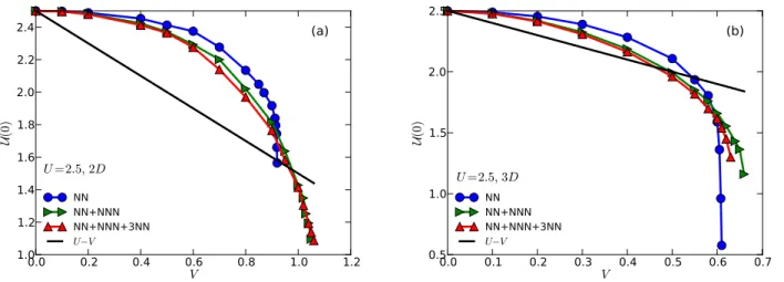
EDMFT provides an elegant means of constructing a model with purely local – though dynamical – interac-tions incorporating the effects of the nonlocal interacinterac-tions in an effective manner. Furthermore, Ref. 34 demon-strated that – at least in the anti-adiabatic limit – a model with dynamical interactions can to a first approx-imation be thought of as a model with static interac-tions corresponding to the zero-frequency limit of the dy-namical ones and a renormalized one-body Hamiltonian. These facts motivate a comparison of the zero-frequency limit of the effective dynamical interaction with attempts in the literature of constructing low-energy Hamiltoni-ans with effective local static interactions, incorporating some of the screening effects stemming from longer range interactions. In Ref.23, it was shown that the best Hub-bard model with purely local interactions mimicking the physics of a model with long-range interactions is one with modified local interactions. “Best” is here defined in the sense of the Peierls-Feynman-Bogoliubov variational principle, leading to a free energy closest to the one of the original system. The result is an effective interaction where the bare interaction U is modified by a weighted average of the nonlocal interaction matrix elements Vij:
Ueff = U + 1 2 X i6=j,σ,σ′ Vij ∂Ueffhniσnjσ′i P l∂Ueffhnl↑nl↓i . (21)
Here, the sums are over lattice sites and spins, and hniσnjσ′i denotes the density-density correlator between
0.0 0.2 0.4 0.6 0.8 1.0 1.2 V 1.0 1.2 1.4 1.6 1.8 2.0 2.2 2.4 U( 0) U =2.5, 2D (a) NN NN+NNN NN+NNN+3NN U−V 0.0 0.1 0.2 0.3 0.4 0.5 0.6 0.7 V 0.5 1.0 1.5 2.0 2.5 U( 0) U =2.5, 3D (b) NN NN+NNN NN+NNN+3NN U−V
FIG. 7. (Color online) Comparison of the effective static interaction U(0) and the simple estimate U − V [see Eq. (22)]. (a) Results for the 2D model with U = 2.5. (b) Results for the 3D model with U = 2.5.
sites i and j. Assuming that a variation of U leads to a displacement of charge only to the nearest neighbor sites, charge conservation leads to a further simplifica-tion. Eq. (21) then reduces to
Ueff= U − V01, (22)
that is, screening by nonlocal interactions results in a simple reduction of the onsite interaction by the nearest neighbor one. Numerical calculations for graphene, sil-icene and benzene in Ref.23indeed found values for the effective interactions close to the simple estimate given by Eq. (22). Inspection of the calculations of Ref. 15
for an extended Hubbard model in two dimensions with NN interactions reveals another interesting aspect: in these calculations screening was found to be strongly de-pendent on the regime, with barely any screening in the Mott phase (as expected) but a strong reduction of the effective local interaction in the correlated metal. In-terestingly, however, the simple estimate of Eq. (22) was found to provide a lower bound with Ueffcoming closer to
U − V01or U depending on the proximity to the metallic
or Mott phase, respectively.
Here, we address the question of the generic character of this observation. In Fig.7, we plot the static part of the effective local interaction obtained from EDMFT as a function of V . As expected, this quantity is strongly reduced when approaching the phase boundary to the CO phase where strong charge fluctuations dominate. In the two-dimensional case with onsite and NN interactions, the effective interaction remains bounded by Eq. (22), while for longer-ranged interactions, U(0) drops below this bound as one approaches the phase boundary. In three dimensions we find a drastic drop of the effective interaction even for the NN case, invalidating any simple estimate. Some of the differences between the 2D and 3D results are presumably due to the fact that the 2D system is closer to the Mott transition.
5. Local spectral properties
We focus on three characteristic regions in the phase diagrams: the FL metallic phase, the MI phase, and the metallic region between the CO and MI phases (or “triangle zone” in between the Vc(U ) and Uc(V ) lines).
We computed the local spectral functions in these zones via analytical continuation of the impurity Green’s func-tion G(τ ). For the calculafunc-tions, we use the method de-scribed in Sec. II C, with the bosonic factor B(τ ) ob-tained from the maximum entropy result for ImU(ν).31,33
In the calculations of B(τ ), we introduced a cutoff at small frequencies to prevent an unphysical divergence of ImU(ν)/ν2 [see insets in Fig. 5(e) and (f)]. The
spec-tral functions A(ω) for the square lattice are displayed in the top panels of Fig.8, while those for the simple cubic lattice are shown in the bottom panels.
We found that the screening effects resulting from long range intersite interactions affect the impurity spec-tral functions in several ways. In the FL regime, the onsite interaction is weak. The major effect of longer range intersite interactions is to transfer spectral weight from the Hubbard bands to the quasiparticle peak, and to small satellites, which are shifted from the Hubbard bands by roughly the effective screening frequency ν0. In
the triangle zone, where the onsite interaction is mod-erate, the longer range intersite interactions can trig-ger an insulator-metal phase transition. Let’s look at Fig.8(e), which illustrates the evolution of the spectral functions across such a metal-insulator transition. For the NN case, the system is an insulator with sharp Hub-bard bands and sizable gap. However, for the NN + NNN case, spectral weight appears at the Fermi level, which indicates a strongly renormalized metallic state. While the Hubbard bands are smeared out, their position is al-most unchanged. When the 3NN intersite interaction is added, the system turns into a good metal with a large
0.0 0.1 0.2 0.3 0.4 0.5 0.6 -6 -4 -2 0 2 4 6 Intensity (a.u) Frequency (a) U = 2.5, V = 0.8 NN + NNNNN NN + NNN + 3NN 0.0 0.1 0.2 0.3 0.4 0.5 0.6 -6 -4 -2 0 2 4 6 Intensity (a.u) Frequency (c) U = 3.0, V = 1.5 NN + NNNNN NN + NNN + 3NN 0.0 0.1 0.2 0.3 0.4 0.5 0.6 -6 -4 -2 0 2 4 6 Intensity (a.u) Frequency (e) U = 2.7, V = 1.0 NN + NNNNN NN + NNN + 3NN 0.0 0.1 0.2 0.3 0.4 0.5 0.6 -6 -4 -2 0 2 4 6 Intensity (a.u) Frequency (b) U = 2.5, V = 0.6 NN + NNNNN NN + NNN + 3NN 0.0 0.1 0.2 0.3 0.4 0.5 0.6 -6 -4 -2 0 2 4 6 Intensity (a.u) Frequency (d) U = 3.6, V = 1.5 NN + NNNNN NN + NNN + 3NN 0.0 0.1 0.2 0.3 0.4 0.5 0.6 -6 -4 -2 0 2 4 6 Intensity (a.u) Frequency (f) U = 3.2, V = 0.8 NN + NNNNN NN + NNN + 3NN
FIG. 8. (Color online) Spectral functions at selected points for the single-band half-filled extended Hubbard model solved by EDMFT. (a), (c), and (e) Results for the square lattice. (b), (d), and (e) Results for the simple cubic lattice. The parameters are as follows: (a) Metallic region, U = 2.5 and V = 0.8; (b) Metallic region, U = 2.5 and V = 0.6; (c) Mott insulating region, U = 3.0 and V = 1.5; (d) Mott insulating region, U = 3.6 and V = 1.5; (e) “Triangle” zone, U = 2.7 and V = 1.0; (f) “Triangle” zone, U = 3.2 and V = 0.8. The impurity spectral functions are obtained using the analytical continuation method proposed in Ref.31.
quasiparticle peak and the Hubbard bands are shifted to higher energy. In the MI phase in which the onsite interaction is strong, the spectral functions are less af-fected by longer range intersite interactions. It seems that the longer range intersite interactions do not signifi-cantly shrink the gaps. The main effect is to redistribute the weight within the Hubbard bands. At the begin-ning, the upper and lower Hubbard bands are broad and smooth. When longer range intersite interactions are in-cluded, the Hubbard bands turn sharper and thinner, and spectral weight is transfered to the edges of the gap and high-frequency features [see Fig.8(d)].
As mentioned before, the structures in ImU(ν)/ν2
pro-duce satellites in the local spectral functions A(ω). For example, the screening modes displayed in Fig.5(e) and (f) explain the broad tails in the energy range |ω| & 2 in Fig.8(a) and (b).
6. Away from half-filling
Having identified the dominant screening modes in the half-filled system and their interpretation in terms of the spectral function, it is interesting to look also at the evo-lution of these quantities away from half-filling. In this section, we present some results for the 2D and 3D lat-tices with onsite and NN intersite interactions. First, we show the phase diagrams for fixed U in the space of V and δµ = µ − U/2. In the 2D (3D) case we choose U = 2.4 and U = 3.6 (U = 2.5 and U = 3.6). For the smaller
onsite interaction, the system at half-filling (δµ = 0) and small enough V is metallic, while for the larger U it is Mott insulating. As the filling of the metallic system is increased, the phase boundary to the CO phase shifts to larger V , i.e., in the small-U regime, the CO instability is a nesting-type phenomenon. We also plot, as dashed lines, the location where the screened interaction W (0) changes sign. We note that this W (0) = 0 line is very different from the FL-CO phase boundary. In the heav-ily doped region, one can still obtain a stable metallic solution even though W (0) < 0.
The situation is quite different for the larger U , where the half-filled solution is either MI or CO. Here, the MI solution is destabilized by doping. In the 3D case, one observes a transition into a doped metal phase for V . 1.0, while in the 2D system, a similar transition occurs for V . 2.0. We note that the phase diagrams of the 2D/3D system are qualitatively very similar to those of the Holstein-Hubbard model.25
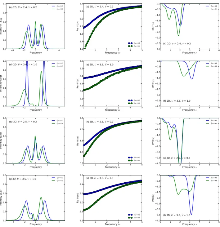
Both the electron spectral function and the screened interaction depend sensitively on δµ. Some representa-tive results are shown in Fig.10. For δµ > 0, the elec-tron spectral function (left panels) becomes asymmetric. In the metallic phase, the quasiparticle peak grows and shifts closer to the upper Hubbard band, while in the in-sulating phase, the gap shrinks due to a broadening of the lower Hubbard band. These changes in the electron spectral function qualitatively explain the changes in the bosonic spectra (right panels). In the metallic case, the main effect of increasing δµ is a growing low-energy
fea-0.0 0.2 0.4 0.6 0.8 1.0 δµ 0.2 0.4 0.6 0.8 1.0 V CO FL (a) 2D, U = 2.4 0.0 0.2 0.4 0.6 0.8 1.0 δµ 0.2 0.4 0.6 0.8 1.0 V CO FL (b) 3D, U = 2.5 0.0 0.2 0.4 0.6 0.8 1.0 1.2 1.4 δµ 0.0 0.5 1.0 1.5 2.0 2.5 3.0 3.5 V MI CO FL (c) 2D, U = 3.6 0.0 0.2 0.4 0.6 0.8 1.0 δµ 0.0 0.5 1.0 1.5 2.0 2.5 V MI CO FL (d) 3D, U = 3.6
FIG. 9. (Color online) V -µ phase diagrams for the single-band extended Hubbard model with NN interactions, determined by EDMFT calculations. Here δµ = µ − U/2. Panels (a) and (c) show results for the 2D square lattice which at half-filling is in the FL or MI regime. Panels (b) and (d) show similar results for the 3D simple cubic lattice. The black dashed lines in (a) and (b) show the location of W (0) = 0, i.e. on the right side of this boundary, the static screened interaction is negative.
ture in ImW (ν). This can be explained by the larger number of states in the quasiparticle band. In the Mott insulating case, where the bosonic spectra for the half-filled system show a single peak at an energy given by the gap, the shrinking of the gap with increasing δµ leads to a broadening and shift of this peak to lower energies. In the 3D case, where the gap size for δµ = 0.6 is small and elec-tron spectral function has a peak at the lower gap edge, we also find a low-energy mode in ImW (ν) which is asso-ciated with transitions between this peak and the upper Hubbard band. Since the low-energy mode in ImW (ν) produces the largest screening effect, it is not surprising that increasing δµ has a large effect on the screened in-teraction (middle panels). As we saw in Fig. 9 (dashed line), in the metallic phase, doping quickly leads to an overscreening of the local interaction.
B. GW + EDMFT results
In this subsection, we present the GW + EDMFT re-sults. Since the computational cost of fully self-consistent GW + EDMFT calculations is much higher than in the case of EDMFT calculations, we do not map out the whole U -V phase diagram. Instead, we performed GW + EDMFT calculations for selected U and V parameters. As a starting point for the self-consistent GW + EDMFT calculation, we used the converged EDMFT results.
1. Nonlocal and local self-energy and polarization
The GW + EDMFT method incorporates nonlo-cal correlations by adding the nonlononlo-cal components of the GW self-energy and polarization functions to the EDMFT result.6,7,14,15 Hence, the GW + EDMFT
frequency-−4 −2 0 2 4 Frequency 0.0 0.2 0.4 0.6 0.8 1.0 In te nsi ty (a .u ) (a) 2D, U = 2.4, V = 0.2 δµ =0.0δµ =0.4 0 1 2 3 4 5 Frequency iν 1.2 1.4 1.6 1.8 2.0 2.2 2.4 R e W (i ν) (b) 2D, U = 2.4, V = 0.2 δµ =0.0 δµ =0.4 0 1 2 Frequency ν3 4 5 6 −4.0 −3.5 −3.0 −2.5 −2.0 −1.5 −1.0 −0.5 0.0 Im W (ν ) (c) 2D, U = 2.4, V = 0.2 δµ =0.0 δµ =0.4 −4 −2 0 2 4 Frequency 0.0 0.2 0.4 0.6 0.8 1.0 In te nsi ty (a .u ) (d) 2D, U = 3.6, V = 1.0 δµ =0.0δµ =0.6 0 1 2 3 4 5 Frequency iν 3.0 3.1 3.2 3.3 3.4 3.5 3.6 R e W (i ν) (e) 2D, U = 3.6, V = 1.0 δµ =0.0 δµ =0.6 0 1 2 3 4 5 6 Frequency ν −4.0 −3.5 −3.0 −2.5 −2.0 −1.5 −1.0 −0.5 0.0 Im W (ν ) (f) 2D, U = 3.6, V = 1.0 δµ =0.0 δµ =0.6 −4 −2 0 2 4 Frequency 0.0 0.2 0.4 0.6 0.8 1.0 In te nsi ty ( a. u) (g) 3D, U = 2.5, V = 0.2 δµ =0.0δµ =0.4 0 1 2 3 4 5 Frequency iν 0.5 1.0 1.5 2.0 2.5 R e W (i ν) (h) 3D, U = 2.5, V = 0.2 δµ =0.0 δµ =0.4 0 1 2 Frequency ν3 4 5 6 −4.0 −3.5 −3.0 −2.5 −2.0 −1.5 −1.0 −0.5 0.0 Im W (ν ) (i) 3D, U = 2.5, V = 0.2 δµ =0.0 δµ =0.4 −4 −2 0 2 4 Frequency 0.0 0.2 0.4 0.6 0.8 1.0 In te nsi ty ( a. u) (j) 3D, U = 3.6, V = 1.0 δµ =0.0δµ =0.6 0 1 2 3 4 5 Frequency iν 2.6 2.8 3.0 3.2 3.4 3.6 R e W (i ν) (k) 3D, U = 3.6, V = 1.0 δµ =0.0 δµ =0.6 0 1 2 3 4 5 6 Frequency ν −4.0 −3.5 −3.0 −2.5 −2.0 −1.5 −1.0 −0.5 0.0 Im W (ν ) (l) 3D, U = 3.6, V = 1.0 δµ =0.0 δµ =0.6
FIG. 10. (Color online) Spectral functions for the Hubbard model with NN interactions away from half-filling. (a)-(f) Results for the square lattice. (g)-(i) Results for the cubic lattice. In the left column, the impurity spectral functions A(ω) are shown. In the middle and right columns, we show the screened interaction W (iν) and corresponding ImW (ν). The parameters are as follows: (a)-(c) U = 2.4, V = 0.2, 2D lattice. (d)-(f) U = 3.6, V = 1.0, 2D lattice. (g)-(i) U = 2.5, V = 0.2, 3D lattice. (j)-(l) U = 3.6, V = 1.0, 3D lattice.
dependent but also momentum-dependent.
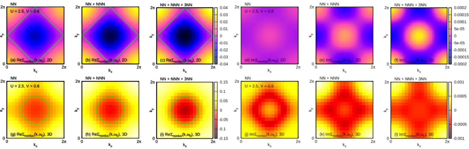
In Fig.11the nonlocal parts of the self-energy for the lowest Matsubara frequency ω0 are shown. These data
have been obtained using Eq. (10). For the square lat-tice, we plot Σnonloc(k, iω0) for kx and ky ∈ [0, 2π]. In
the case of the simple cubic lattice, we show a cut of Σnonloc(k, iω0) in the kz= 0 plane. Consistent with
pre-vious GW + EDMFT calculations for the square lattice
with NN interations,15 we find that the GW
contribu-tion to the imaginary part of the nonlocal self-energy is negligible with respect to the local self-energy. The real part of the nonlocal self-energy is relatively large away from the EDMFT Fermi surface, but does not alter this Fermi surface. Longer range interactions do increase the k-dependence, but they do not significantly affect the conclusion that the k-dependence of the self-energy
0 2π kx 0 2π ky U = 2.5, V = 0.8 NN (a) ReΣnonloc(k,ω0), 2D 0 2π kx 0 2π ky U = 2.5, V = 0.8 NN (a) ReΣnonloc(k,ω0), 2D 0 2π kx 0 2π ky NN + NNN (b) ReΣnonloc(k,ω0), 2D 0 2π kx 0 2π ky NN + NNN (b) ReΣnonloc(k,ω0), 2D 0 2π kx 0 2π ky -0.04 -0.03 -0.02 -0.01 0 0.01 0.02 0.03 0.04 NN + NNN + 3NN (c) ReΣnonloc(k,ω0), 2D 0 2π kx 0 2π ky NN + NNN + 3NN (c) ReΣnonloc(k,ω0), 2D 0 2π kx 0 2π ky NN U = 2.5, V = 0.8 (d) ImΣnonloc(k,ω0), 2D 0 2π kx 0 2π ky NN + NNN (e) ImΣnonloc(k,ω0), 2D 0 2π kx 0 2π ky -0.0002 -0.00015 -0.0001 -5e-05 0 5e-05 0.0001 0.00015 0.0002 NN + NNN + 3NN (f) ImΣnonloc(k,ω0), 2D 0 2π kx 0 2π ky NN U = 2.5, V = 0.6 (g) ReΣnonloc(k,ω0), 3D 0 2π kx 0 2π ky NN U = 2.5, V = 0.6 (g) ReΣnonloc(k,ω0), 3D 0 2π kx 0 2π ky NN + NNN (h) ReΣnonloc(k,ω0), 3D 0 2π kx 0 2π ky NN + NNN (h) ReΣnonloc(k,ω0), 3D 0 2π kx 0 2π ky -0.15 -0.1 -0.05 0 0.05 0.1 0.15 NN + NNN + 3NN (i) ReΣnonloc(k,ω0), 3D 0 2π kx 0 2π ky NN + NNN + 3NN (i) ReΣnonloc(k,ω0), 3D 0 2π kx 0 2π ky NN U = 2.5, V = 0.6 (j) ImΣnonloc(k,ω0), 3D 0 2π kx 0 2π ky NN + NNN (k) ImΣnonloc(k,ω0), 3D 0 2π kx 0 2π ky -0.001 -0.0005 0 0.0005 0.001 NN + NNN + 3NN (l) ImΣnonloc(k,ω0), 3D
FIG. 11. (Color online) Σnonloc(k, iω0) for the extended Hubbard model from GW + EDMFT. (a)-(f) Results for the square
lattice, U = 2.5, V = 0.80. (g)-(l) Results for the simple cubic lattice, U = 2.5, V = 0.60. We only show the kz = 0 plane.
(a)-(c) and (g)-(i) ReΣnonloc(k, iω0). (d)-(f) and (j)-(l) ImΣnonloc(k, iω0). The green curves in (a)-(c) and (g)-(i) panels denote
the EDMFT Fermi surface.
-2.0 -1.8 -1.6 -1.4 -1.2 -1.0 -0.8 -0.6 -0.4 -0.2 0.0 0.2 0.4 0.6 0.8 1.0 Im Σ (i ω ) Frequency iω (a) 2D NN, EDMFT NN + NNN, EDMFT NN + NNN + 3NN, EDMFT NN, GW + EDMFT NN + NNN, GW + EDMFT NN + NNN + 3NN, GW + EDMFT -0.9 -0.8 -0.7 -0.6 -0.5 -0.4 -0.3 -0.2 -0.1 0.0 0.0 0.2 0.4 0.6 0.8 1.0 Im Σ (i ω ) Frequency iω (b) 3D NN, EDMFT NN + NNN, EDMFT NN + NNN + 3NN, EDMFT NN, GW + EDMFT NN + NNN, GW + EDMFT NN + NNN + 3NN, GW + EDMFT
FIG. 12. (Color online) Imaginary part of the local self-energy function ImΣ(iω) for the extended Hubbard model solved with EDMFT and GW + EDMFT. (a) Results for the square lattice, U = 2.5 and V = 0.8. (b) Results for the simple cubic lattice, U = 2.5 and V = 0.6.
both for the 2D and 3D lattice models is not very strong in the GW + EDMFT scheme. Even in the vicinity of the Mott transition (for instance, U = 2.5 and V = 0.8 for the square lattice is very close to the Mott transi-tion, see Fig. 2), the momentum differentiation is weak. This result is in contrast to the strong momentum depen-dence observed in the self-energy functions obtained from dynamical cluster approximation (DCA)35,36 and
cellu-lar dynamical mean-field theory (CDMFT)37,38
calcula-tions for the two-dimensional Hubbard model as one ap-proaches the Mott transition. This discrepancy suggests that additional nonlocal diagrams, such as ladder dia-grams, should be included to provide a better description of the momentum dependence of the self-energy functions (and other k-dependent quantities).
As for the nonlocal polarization function for the first bosonic Matsubara frequency Πnonloc(k, iν = 0) (not
shown in this figure), we observe a stronger momentum
dependence, especially when one approaches the charge-ordering transition.15However, it seems that longer range
intersite interactions do not enhance this k-dependence prominently, which is contrary to the trend found for the nonlocal self-energy.
Finally, we plot in Fig. 12 some typical local self-energies in the FL phase. |ImΣ(iω0)| is considerably
en-hanced in the GW + EDMFT calculations, compared to the EDMFT result. These observations show that local correlations become stronger if the k-dependent GW con-tributions are added to the self-energy and polarization functions in the self-consistency loop. More evidence for this change will be presented in the following section. In Fig. 12, we also compare the local self-energies for in-tersite interactions of different range. The effect of the longer ranged interactions is to reduce the self-energy. In the calculations with long range interactions and nonlo-cal self-energies we thus have a competition between the
additional screening from long range interactions, which leads to weaker correlation effects, and the momentum dependence, which enhances local correlations. The lat-ter effect seems to be dominant.
2. Screened and retarded interactions
As we have seen in the previous subsection, the GW + EDMFT scheme not only adds nonlocal contributions to the self-energy Σ(k, iωn) and polarization Π(k, iνn),
but it also affects the local quantities through the self-consistency loop.15 Figure 13 shows the fully screened
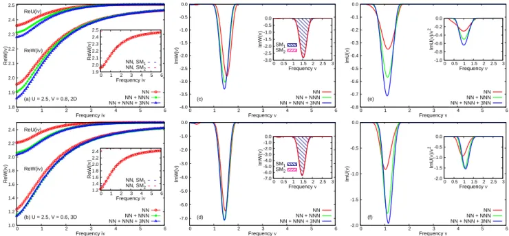
local interaction ReW (iν) and partially screened inter-action ReU(iν), together with the corresponding spectral functions ImW (ν) and ImU(ν), for the square lattice and simple cubic lattice in the FL metallic state. The related EDMFT data have been plotted in Fig.5 and analyzed in Sec.III A. Again, our results are consistent with previ-ous GW + EDMFT studies for the 2D and 3D extended Hubbard model if available.7,15
Compared to the EDMFT result, both ReW (iν = 0) and ReU(iν = 0) are greatly enhanced [see Fig. 13(a) and (b)], while |ImG(iω0)| (not shown in these figures)
is reduced. This indicates that the local interactions are stronger in GW + EDMFT than in EDMFT, i.e., that the screening effect is weaker. This can be understood in the following way:15 In the EDMFT approach, all of
the screening and correlation effects are absorbed into the local self-energy. However, in the framework of GW + EDMFT, some of these effects are carried by the non-local self-energy. In other words, the screening between local and nonlocal quantities is redistributed in the GW + EDMFT scheme, and the result of this is that the local interaction becomes less screened. Let us also mention that Nomura et al.39have shown that the nonlocal
polar-ization induces an anti-screening effect, which competes with the screening effect caused by the long range in-tersite interactions. Anyhow, the interplay between the local and nonlocal self-energy and polarization in GW + EDMFT leads, after self-consistency, to a weaker screen-ing effect.
Another interesting observation is that the ImW (ν) and ImU(ν) spectra extracted from the self-consistent GW + EDMFT calculations [see Fig. 13(c)-(f)] ex-hibit a single-hump structure, whereas the corresponding EDMFT results yield a two-hump structure [see Fig.5 (c)-(f)]. Once again, we have fitted ImW (ν) with multiple Gaussians to extract the positions and weights of the dominant SMs. It seems that the ImW (ν) spectra ob-tained from the GW + EDMFT calculations feature only one medium-frequency SM (∼ 1.5 eV), while the low-frequency SMs (∼ 0.5 eV) are extremely weak and the high-frequency SMs (2 ∼ 3 eV) previously identified in the EDMFT results have disappeared. As for the ImU(ν) spectra, analogous characteristics are observed. Since the satellite structures of the local spectral function A(ω) are determined by the function ImU(ν)/ν2,32 we conclude
that the high-frequency features of A(ω) will be different in the GW + EDMFT calculations, and more specifi-cally that the satellites will be at lower energy. Though we only present results for the FL metallic phase in this figure, those for the Mott phase and the strongly corre-lated metal phase between the MI and CO states exhibit the same trend (see also Tab.I).
Next, we consider the influence of longer range inter-site interactions on the static screened and retarded in-teractions obtained with the GW + EDMFT scheme. TableI also shows data collected from GW + EDMFT calculations. Once more, we see that ReU(ν = 0) and ReW (ν = 0) are reduced, and |ImG(iω0)| (not shown
in the Table) is enhanced if longer range intersite teractions are present. The effects of longer range in-teractions and nonlocal correlations compete with each other: the longer range intersite interaction tends to en-hance the screening and make the system less correlated, while including the GW nonlocal self-energies and po-larizations has the opposite effect. The latter effect is dominant. From Fig.13(e) and (f), we can see that the weight of the hump in the ImU(ν) spectra increases if longer range intersite interactions are added which means a larger screening effect. However, interestingly, the ef-fective screening frequency ν0 is only little affected by
the range of the interaction within the GW + EDMFT approach, which is also seen in Tab.I.
3. Local spectral properties
The top panels of Fig. 14 show some typical spec-tral functions for the square lattice obtained by GW + EDMFT. Similar results for the simple cubic lattice are shown in the bottom panels. Here we consider the FL metallic state, MI state, and the “triangle” zone in the U − V phase diagrams. Since the parameter values are the same, one can directly compare these spectra to the EDMFT results as shown in Fig.8. Consistent with the previous discussion, within the GW + EDMFT scheme, the quasiparticle peak is greatly reduced, and the upper and lower Hubbard bands become more pronounced. For instance, let us focus on the “triangle” zone for the square lattice (parameters U = 2.7 and V = 1.0). The EDMFT local spectral function shows considerable weight at the Fermi level, i.e., the system is metallic [see Fig. 8(e), for the NN + NNN case]. However, the corresponding GW + EDMFT spectral function has almost no weight at ω = 0, which means that it is close to or even in the MI phase [see Fig. 14(e), for the NN + NNN case]. From this fact, we conclude that there exists a small dif-ference between the FL-MI phase boundaries calculated with EDMFT and GW + EDMFT, respectively, and that the MI region in the latter case should be larger.
The influence of longer range intersite interactions on the local spectral functions A(ω) is very similar to the EDMFT case. Namely, longer range intersite interac-tions enhance the quasiparticle peak and shift spectral
1.8 1.9 2.0 2.1 2.2 2.3 2.4 2.5 0 1 2 3 4 5 6 ReW(i ν ) Frequency iν (a) U = 2.5, V = 0.8, 2D ReW(iν) ReU(iν) NN NN + NNN NN + NNN + 3NN 1.9 2.0 2.1 2.2 2.3 2.4 2.5 0 1 2 3 4 5 6 ReW(i ν ) Frequency iν NN, SM1 NN, SM2 -4.0 -3.5 -3.0 -2.5 -2.0 -1.5 -1.0 -0.5 0.0 0 1 2 3 4 5 6 ImW( ν ) Frequency ν (c) NN NN + NNN NN + NNN + 3NN -3.0 -2.5 -2.0 -1.5 -1.0 -0.5 0.0 0 0.5 1 1.5 2 2.5 3 ImW( ν ) Frequency ν SM1 SM2 -0.8 -0.7 -0.6 -0.5 -0.4 -0.3 -0.2 -0.1 0.0 0 1 2 3 4 5 6 ImU( ν ) Frequency ν (e) NN NN + NNN NN + NNN + 3NN -1.0 -0.8 -0.6 -0.4 -0.2 0.0 0 0.5 1 1.5 2 2.5 3 ImU( ν )/ ν 2 Frequency ν 1.0 1.2 1.4 1.6 1.8 2.0 2.2 2.4 0 1 2 3 4 5 6 ReW(i ν ) Frequency iν (b) U = 2.5, V = 0.6, 3D ReW(iν) ReU(iν) NN NN + NNN NN + NNN + 3NN 1.2 1.4 1.6 1.8 2.0 2.2 2.4 0 1 2 3 4 5 6 ReW(i ν ) Frequency iν NN, SM1 NN, SM2 -7.0 -6.0 -5.0 -4.0 -3.0 -2.0 -1.0 0.0 0 1 2 3 4 5 6 ImW( ν ) Frequency ν (d) NN NN + NNN NN + NNN + 3NN -7.0 -6.0 -5.0 -4.0 -3.0 -2.0 -1.0 0.0 0 0.5 1 1.5 2 2.5 3 ImW( ν ) Frequency ν SM1 SM2 -2.0 -1.5 -1.0 -0.5 0.0 0 1 2 3 4 5 6 ImU( ν ) Frequency ν (f) NN NN + NNN NN + NNN + 3NN -2.0 -1.5 -1.0 -0.5 0.0 0 0.5 1 1.5 2 2.5 3 ImU( ν )/ ν 2 Frequency ν
FIG. 13. (Color online) Real part of the fully screened interactions ReW (iν) and partially screened interaction ReU(iν), imaginary part of the real frequency fully screened interaction ImW (ν) and partially screened interactions ImU(ν) for the extended Hubbard model solved by GW + EDMFT. (a), (c) and (e) Results for the square lattice, U = 2.5 and V = 0.8. (b), (d) and (e) Results for the simple cubic lattice, U = 2.5 and V = 0.6. In this figure, SM means screening mode. In the insets of panels (a) and (b), the SM-resolved ReW (iν), together with full ReW (iν) are shown for the NN case. In the (c) and (d) panels, the ImW (ν) for the NN case is approximated by Gaussian-type functions. The fitted results are shown in the insets. Each Gaussian peak corresponds to a SM. The insets in panels (e) and (f) show the ImU(ν)/ν2
functions. Here ImW (ν) and ImU(ν) are extracted using a modified maximum entropy method. See AppendixBfor more details.
0.0 0.1 0.2 0.3 0.4 0.5 0.6 -6 -4 -2 0 2 4 6 Intensity (a.u) Frequency (a) U = 2.5, V = 0.8 NN + NNNNN NN + NNN + 3NN 0.0 0.1 0.2 0.3 0.4 0.5 0.6 -6 -4 -2 0 2 4 6 Intensity (a.u) Frequency (c) U = 3.0, V = 1.5 NN + NNNNN NN + NNN + 3NN 0.0 0.1 0.2 0.3 0.4 0.5 0.6 -6 -4 -2 0 2 4 6 Intensity (a.u) Frequency (e) U = 2.7, V = 1.0 NN + NNNNN NN + NNN + 3NN 0.0 0.1 0.2 0.3 0.4 0.5 0.6 -6 -4 -2 0 2 4 6 Intensity (a.u) Frequency (b) U = 2.5, V = 0.6 NN + NNNNN NN + NNN + 3NN 0.0 0.1 0.2 0.3 0.4 0.5 0.6 -6 -4 -2 0 2 4 6 Intensity (a.u) Frequency (d) U = 3.6, V = 1.5 NN + NNNNN NN + NNN + 3NN 0.0 0.1 0.2 0.3 0.4 0.5 0.6 -6 -4 -2 0 2 4 6 Intensity (a.u) Frequency (f) U = 3.2, V = 0.8 NN + NNNNN NN + NNN + 3NN
FIG. 14. (Color online) Spectral functions at selected points for the single-band half-filled extended Hubbard model solved by GW + EDMFT. (a), (c), and (e) Results for the square lattice. (b), (d), and (e) Results for the simple cubic lattice. The parameters are as follows: (a) Metallic region, U = 2.5 and V = 0.8; (b) Metallic region, U = 2.5 and V = 0.6; (c) Mott insulating region, U = 3.0 and V = 1.5; (d) Mott insulating region, U = 3.6 and V = 1.5; (e) “Triangle” zone, U = 2.7 and V = 1.0; (f) “Triangle” zone, U = 3.2 and V = 0.8. The impurity spectral functions are obtained using the analytical continuation method proposed in Ref.31.