Design of a person tracking algorithm for the intelligent room

(1)

Design of a -Person Tracking Algorithm

for the Intelligent Room

by

Gregory Andrew Klanderman

Submitted to the Department of Electrical Engineering and Computer Science

in partial fulfillment of the requirements for the degree of

Master of Science in Computer Science and Engineering

at the

MASSACHUSETTS INSTITUTE OF TECHNOLOGY

August 1995

@

Massachusetts Institute of Technology 1995. All rights reserved.

Signature of Author

... . ...

.'...

Department of ilectrical Engineering and Computer Science

August 18, 1995

Certified by ... ...

--

• .

...

W. Eric L. Grimson

Professor of Computer Science

Thesis Supervisor

(71,

Accepted by...

. . .

N.. :

V•e,...

F. R. Morgenthaler

Chairman, epartmental ommittee on Graduate Students

;.LASAGCHUSEfTS INSIi

Ui-OF TECHNOLOGY

~nr

NOV

0

2 1995

(2)

(3)

Design of a Person Tracking Algorithm

for the Intelligent Room

by

Gregory Andrew Klanderman

Submitted to the Department of Electrical Engineering and Computer Science on August 18, 1995, in partial fulfillment of the

requirements for the degree of

Master of Science in Computer Science and Engineering

Abstract

In order to build a room which can monitor the activities of its occupants and assist them naturally in the tasks they are performing, it is first necessary to be able to determine the locations and identities of its occupants. In this thesis, we analyze several algorithms proposed for visually tracking people interacting in such a computer-monitored "intelligent room". Through both experiments on real data and theoretical analysis of the algorithms, we will characterize the strengths and weaknesses of these algorithms. Given this analysis, we will discuss the implications for building a person tracking system using some combination these algorithms. We finish by proposing further experiments and an algorithm to solve the person tracking problem. This algorithm will form the basis for higher-level visual identification and gesture recognition for the Intelligent Room currently being built at the MIT Artificial Intelligence Laboratory.

Thesis Supervisor: W. Eric L. Grimson Title: Professor of Computer Science

(4)

(5)

Acknowledgments

I would like to thank my advisor Eric Grimson for all the direction and support he has provided which were essential to the completion of this work. I would also like to thank Tom's Lozano-P6rez for his direction while Eric was on sabbatical and for pushing me to work hard in the early stages of this work. In addition, I have benefited greatly from many conversations with the members of both the HCI and WELG groups. My officemates Pamela Lipson and Aparna Lakshmi Ratan certainly deserve many thanks for all their help and for putting up with me during the last three years. And of course, Dan Huttenlocher cannot be thanked enough for getting me interested in computer vision and for always looking out for me. Special thanks also go to Sajit Rao, Miguel Schneider, Jae Noh, and William Rucklidge who generously provided code which I used extensively. My many friends at the AI Lab, MIT, and elsewhere must also be thanked. Their humor and the many diversions they provided somehow kept me sane throughout this endeavor. Finally and most importantly, I would like to thank my family without whose constant support throughout my entire life I could never have gotten here.

This report describes research done at the Artificial Intelligence Laboratory of the Massachusetts Institute of Technology, and was funded in part by the Advanced Research Projects Agency of the Department of Defense under Image Understanding contract number N00014-94-01-0994 and the Air Force Office of Sponsored Research under contract number F49620-93-1-0604.

(6)

(7)

Chapter 1 Introduction

At the MIT Artificial Intelligence Laboratory, we have embarked upon building the prototype system for a new paradigm in human-computer interaction. The goal is to eliminate explicit interaction with the computer in favor of a natural, seamless interface with computing resources. This natural interface would make interacting with the computer much like interacting with another human. The interface will take the form of an intelligent room which is able to interpret and augment human activity within the room. With the computer acting as an observer and participant, people in the room will be able to transparently command a vast array of computational and communication resources without even thinking about it. Instead, they will concentrate on solving real problems.

The applications we envision for such a room revolve around collaborative planning, rehearsal, and technical design. For example, a remote doctor assists in a surgery or one or more doctors plan a surgery, rehearsing several scenarios. Augmented reality eyeglass displays show a segmented model of the patient's anatomy. Tactile feedback allows probing of anatomical structures. Hand gestures allow the surgeon to change viewpoint, and voice commands allow him to remove structures to see what is beneath. Intelligent software agents look for relevant information in the patient's history and search for similar cases the doctor has seen.

As another example, in the context of collaborative mechanical design, engineers view a model of the system being designed. Augmented reality glasses automatically highlight different aspects of the design based on the current discussion or background and interests of each participant. As the discussion progresses, 'minutes' are automatically kept containing who said what for future reference. The room keeps track of who has the floor and allows that person to manipulate the shared view and modify the design using natural hand gestures.

The technology needed to build such a room consists of various presentation devices (augmented reality glasses, large screen displays, tactile feedback), intelligent software agents, a perceptual sys-tem to allow natural interaction, and a coordination and control syssys-tem. In this thesis, we are

(10)

interested in building a basic component of the room's perceptual system. The perceptual system has the task of observing the people in the room and understanding what they are doing. It has to locate the occupants, identify them, recognize large and small scale gestures they are making, esti-mate where they are looking, estiesti-mate where they are pointing, determine their facial expressions, and recognize who is leading the discussion (who 'has the floor'). We propose to implement this part of the perceptual functionality visually, using a number of active and passive video cameras placed in the room to observe the occupants. Of course, other non-visual perceptual components will be needed, such as a voice recognition system to allow voice interaction.

This research is concerned with developing a low level person tracking system on which to base the higher lever visual processes of the room. This system will be responsible for tracking the location of each of the room's occupants through time. Since many higher level processes will be using this information, it must be very robust. In this thesis, we present research on the design of such a person tracking system. We will evaluate the performance of three tracking systems on many video sequences to characterize their strengths and weaknesses. Given this analysis, we will discuss the implications for building the person tracking system for the Intelligent Room using some combination these algorithms. We finishing by proposing further experiments and an algorithm to solve the person tracking problem.

1.1 Person Tracking

In order visually to observe people with the goal of understanding their gestures and allowing natural interaction with the computer to take place, we must first know where the people are so we can have some idea of where to look for these gestures. For example, we propose to recognize pointing and other hand and arm gestures, to determine gaze direction and facial expression, and to use face recognition to identify the participants. Since the room is a large and unstructured space with people allowed to come and go, these tasks are much easier if we can constrain the search space

by having a rough idea where to look for arms, hands, and faces as well as how many to expect.

Also, if we can recognize who has the floor (the person leading the discussion), we can direct the computational resources to that person's needs.

Thus, we need a multiple person tracking system to localize each person in the room and track these positions over time. At each time, the system should estimate the pose and location of each person and determine the correspondences with previous estimates. We will refer to determining correspondences as solving the 'person constancy problem'. It is not enough simply to know where people are; we need to know that the person now located at some position is the same one we observed at another location previously. This allows a higher-level process to assist the same person through time as they move around within the room.

(11)

The system must operate in real time and be capable of tracking complex human interactions over very long time periods (ideally, an hour or more). It must be very robust because higher level visual processing will be based on its estimates. Full recovery of the shape of the people in the room is probably unnecessary, however[14, 22]. Even if possible, this would require many orders of magnitude more computation than we can afford. Instead, the position and shape of a participant will be represented retinotopically, as the set of camera pixels comprising the image of that participant. Given the rough localization of each person, higher level process can determine what additional information is necessary for their task.

Figure 1-1 demonstrates the desired behavior of the multiple person tracking system. The figure shows two images from a sequence taken while three occupants were moving around in the room. The time elapsed between the two frames is a few seconds. Rough localization of the people has been accomplished by placing a bounding box around each person's outline in each frame. Further, correspondences between the detected people are represented by each person being given the same label in both frames.

In this thesis we consider only the restricted case of a single, fixed view, wide angle camera ob-serving an area where people are interacting. We are interested in eventually incorporating multiple, possibly active cameras in the room for tracking, but this is outside the scope of the current research. In this context, the tracking system will determine the locations of the people present in each video frame as well as correspondences between the tracked people in consecutive frames.

Why should this tracking be done visually? We could use a pressure sensitive floor or

transpon-ders worn by the occupants, but these would not be able to give a rough segmentation of the people in the scene, just a single reference point. Also, a pressure sensitive floor would not solve the person constancy problem, and would likely be confused by chairs being moved around. Further, we would like to avoid having to instrument the people in the room; anyone should be able to enter and par-ticipate. Our goal is to make the room as non-intrusive as possible. Those who care to may wear enhanced reality glasses, but not all applications would need this technology so we hesitate to require it. Also, other applications of the technology being developed such as analysis of pedestrian traffic would not allow instrumenting each participant. We would like the technology required to be able to be added to an existing room as easily as possible. Requiring the floor to be instrumented with an array of sensors would be a significant impediment to transferring the technology into existing rooms. Finally, the higher level systems seem best solved visually.

1.2 Difficulty

The context of the room provides many constraints on this problem. For example, the only moving things are people or images on computer screens. The screens are in fixed and known locations._I

(12)

Figure 1-1: Example demonstrating the desired behavior of the multiple person tracking system.

(13)

People are usually standing or sitting, and normally are upright. The background is relatively stable and lighting is mostly constant temporally, except for lighting changes and shadows. Most lighting

changes will be computer initiated.

However, there are many difficulties. Keeping in mind the expected use for collaborative design and planning sessions, we expect participants in the room will often be close together and not moving a lot. Segmentation will be difficult with people nearby or occluding each other. People are inherently non-rigid and have many degrees of motion; arms and legs can be moving in very different directions and at different speeds. People may sit or stand still for long periods, then quickly turn around or bend over. Tracking all of these motions can be difficult. The person constancy problem is very difficult; it involves matching many similar non-rigid objects and distinguishing between them over time. When a participant is showing slides, low-lighting conditions may greatly reduce the contrast. Finally, a person gesturing in front of the shared large screen display may be difficult to

track if the image on the screen is also changing.

1.3 Related Work

Much research in computer vision has been done on tracking both feature points and objects. Types of objects tracked vary widely. Tracking systems make various assumptions about the type of object to be tracked, for example whether or not the object is or is not rigid, articulated, or polyhedral. Tracking systems may be based on 3d or 2d models or may not be model based at all.

The basics of feature point tracking seem to be relatively well understood[21]. Correlation based methods which minimize sum of squared differences with respect to translation seem to work quite well in the case of small inter-frame displacements (See [1], for example). The problem of selecting good feature windows to track is more difficult. Obviously it is important that the feature window being tracked correspond to a real point in the world, not a motion boundary or specularity on a glossy surface. Shi and Tomasi[21] developed a promising selection criterion and feature monitoring method to select good features and detect when the template approach has lost the feature. A translation only model of image motion is used when matching from frame to frame, while an affine model is used over longer time periods to monitor if the original feature is still being tracked. Nowlan[17] has used convolutional neural networks to track a hand through hundreds of video frames and identify whether it is open or closed. The tracking system was able to track a number of hands correctly through 99.3 percent of the frames using a correlation based template match.

Lowe [13] has shown good tracking results for articulated polyhedral objects with partial oc-clusion. He uses an integrated treatment of matching and measurement errors, combined with a best-first search. The method handles large frame to frame motions and can track models with many degrees of freedom in real time. This method is probably not applicable to our needs since it

(14)

requires a 3d model of a rigid, articulated object comprised of straight line-segment features. Woodfill and Zabih describe real-time tracking of a single non-rigid object[25]. They use dense motion field estimates based on consecutive frames to propagate a 2d model from frame to frame. The model is a boolean retinotopic map. The camera need not be fixed. At each frame, they adjust the model towards motion or stereo boundaries. They show results of tracking people on a CM-2 parallel computer. Having implemented this algorithm, we are skeptical about propagating optical flow estimates over many frames. Because there is noise in the optical flow computation, these errors get magnified over many frames causing the model to diverge and fill with gaps.

Huttenlocher et al.[10] have developed a model based tracking system based on 2d shape matching using a Hausdorff distance metric which works well. This is one of the algorithms we will be considering and will be described in detail in Section 2.3.

Bascle[2] integrates snake-based contour tracking with region based motion analysis. The motion field within the tracked object is used to estimate an affine motion of the object. This estimate is used to update the B-spline model and guide the initialization of a snake with affine motion constraints for segmentation in the next frame. Next, the affine constraints on the snake are relaxed giving the new object segmentation. Because the snake seeks edge boundaries, it does a good job segmenting the object. However, it requires a good initialization because it only uses edge information. Optical flow does not estimate region boundaries well, as seen by the failures of the Woodfill and Zabih method. But by using the whole region, it does estimate region motion quite precisely. This method has been used to track cars on a highway. It is unclear whether people would move fast enough to break the assumptions of mostly affine motion in our application.

Koller, et al. are also interested in tracking cars on a highway[11]. By using an adaptive

background model, the objects are extracted then adjusted toward high spatial and time gradients. They use a Kalman filter to estimate the affine motion parameters of each object. Since the motion is constrained to the highway and the scene geometry is known, they can determine a depth ordering of the scene and therefore reason about occlusions. Again, it is unclear whether we can make the assumption of affine motion. Also, the ground plane assumption may not be useful to us if there are chairs and tables in the room which could occlude people's feet from view, as we expect to be the case.

Work on tracking people for measuring pedestrian traffic and intrusion detection has been done by Shio[22] and by Makarov[15]. Shio argues against recovery of full 3d structure in favor of 2d translational motion, considering algorithm robustness against noise and changing imaging condi-tions more important than high fidelity. He uses a background subtraction to segment the people from the background. By spatially propagating the motion field and smoothing the motion vectors temporally over a few seconds, the motions of all parts of a single person converge to the same value. Motion regions are then split and merged based on motion direction and a simple

(15)

proba-bilistic model of object shape to give a segmentation of the people. Makarov obtained good results

for intrusion detection using a simple background subtraction on non-thinned edges. He notes that lighting changes are the main cause of false alarms for intrusion detection systems. Because of the prevalence of shadows and reflections in indoor scenes, ordinary background subtraction methods do not perform well. He obtained good results for his algorithm, but tested robustness to lighting change using an artificial additive model which does not effect the image derivatives upon which the edge detector is based except due to saturation.

Maes et al.[14] have developed a system which allows a user to interact with virtual agents. A camera projects an image of the user on a large screen and cartoon-like agents are virtually projected giving a 'magic mirror' effect. The system uses computer vision techniques to segment the user's silhouette and analyze his gestures. Very simple techniques suffice, because of the controlled environment. The constant background and floor and controlled lighting allow simple 'blue screen' subtraction to segment the user. The orientation with respect to the screen is controlled, since you must look at the screen. There is no furniture, making it easy to estimate depth based on the intersection of the ground plane with the user's feet. This system is similar to ours, however we are interested in allowing multiple people to interact in much less constrained environments.

Finally, much speculation exists regarding the form human-computer interaction will take in the future. For example, the video by Sun Microsystems[16] gives their vision. Many aspects of this vision are similar to ours, including multi-media presentation support using visual gesture recognition, speech understanding, enhanced visualization, access to global information, and remote participation.

1.4 Approach

In order to design a multiple person tracking algorithm for the Intelligent Room, we will first analyze three algorithms developed for similar purposes. All are based on having a single fixed camera observing the area in which we wish to allow intelligent interaction with the computer. The first is a correlation based feature tracker, similar to those described in [1], [24], and [21]. The second uses motion information to segment the image into moving objects. This tracker uses some of the ideas discussed in [25] but is greatly simplified. The final algorithm is a model based system employing

2D shape matching using the Hausdorff distance. This algorithm was developed by Huttenlocher,

et al. [10]. Our hope is that the shape matching which it uses will enable us to distinguish between multiple people and solve the person constancy problem for tracking several people.

The planned experiments consist of a number of difficult cases obtained by reasoning about the algorithms and also observing their behavior in many situations. For example, in the motion based algorithm, if the person moves too fast, the search radius in the optical flow step will be too small

(16)

0.8 0.6 U) 0.4 0.2 n

sequence: squares1 run: startS down: 1

0 5 10 15 20 25 30 35 40 45

Image Number

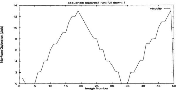
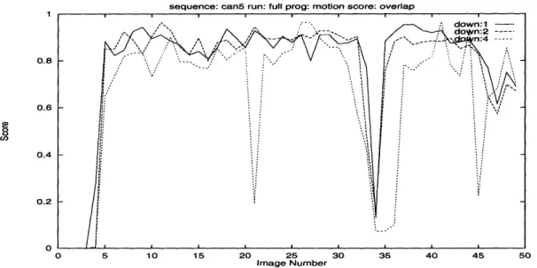
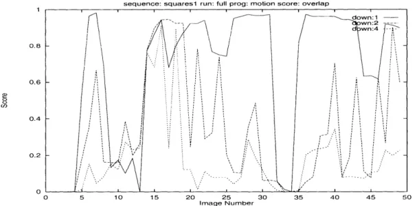
Figure 1-2: Example plot comparing the frame by frame scores of runs of the three algorithms on the full resolution squares sequence.

and the algorithm should fail to find matches. The experiments involve a number of tests of the algorithms tracking simple objects making relatively simple motions as well as tracking real people interacting in the room.

Analysis of the experiments will involve scoring each algorithm's performance on each test video sequence. Ground truth data will allow us to score each algorithm's performance. Using this quantitative analysis as a guide, we can quickly analyze the strengths and failures of each algorithm qualitatively and uncover the reasons for each failure. Based on these failures, we then propose an algorithm that is less susceptible to these conditions.

Figure 1-2 shows an example of the type of quantitative analysis we will be using. Scores for each of the three algorithms we are studying are plotted as a function of image frame number for one of the video sequences we will be using. From the plot it is easy to see when the algorithms are performing well and when they are failing. We will be using this type of analysis extensively in Chapter 4.

The remainder of this thesis is organized as follows: Chapter 2 describes each of the algorithms we will be analyzing in detail. Chapter 3 describes the experimental design, including our image sequences, the experiments we will be doing, quantitative measurement of performance, and analysis. Chapter 4 describes each of our experiments and analyzes the results. Finally, Chapter 5 analyzes the implications of these experimental results for solving the person tracking problem and proposes further experiments and an algorithm to track people.

(17)

Chapter 2 Tracking Algorithms

As we have described previously, we will be analyzing three tracking algorithms and the features of which they make use. By understanding the conditions under which they succeed and fail, we will be able to suggest an algorithm to solve the multiple person tracking problem in the Intelligent Room. We have chosen these algorithms because the underlying features of the algorithms are representative of a wide range of tracking systems. The features used are correlation matching, difference images, optical flow (motion), and shape matching.

2.1 Correlation Based Feature Tracking Algorithm

The first algorithm we will consider is a correlation based feature point tracker. The basic algorithm is very simple and consists of tracking a small patch of an image of the object of interest from frame to frame, looking for the best match of the patch from the previous image in the current image. The particular implementation described was originally developed by Miguel Schneider[20] for an embedded TMS320C30 based vision system. Only minor changes were made in converting it to run

on a UNIX platform.

Correlation based feature trackers are quite common for computer vision applications (see [1], [24], and [21]). They are also among the simplest tracking algorithms. The general framework for a correlation based feature tracker is shown in Figure 2-1. At each step, we first locate the feature being tracked in the current frame. Using the image patch surrounding the feature in the previous image as a template, we look in a region of the current image around the predicted new location for the best match with the template. This predicted location may be based on the previous trajectory, among other things. Using the best match location, we then update the template and trajectory information. Although the matching we use is based on minimizing a sum of squared differences, it is essentially equivalent to maximizing the correlation and hence we will refer to this algorithm as the correlation based feature tracker.

(18)

Figure 2-1: Correlation based feature-point tracker

Let Mt I [i, j] be the N x N feature template from time t - 1. For convenience, let N = 2Rp + 1

where Rp is the patch radius and let the i and j indices of Mt-1 range from -Rp to Rp. This choice of coordinates allows the center of the patch to have coordinates (0, 0) and we designate this position the feature's location. Usually the patch is rather small in relation to the whole object being tracked and is centered on some local feature of that object. Given a new image It [i, j] at time t, we search for the best match for the model patch Mt-1 in the region of the image It of radius

Rs surrounding the predicted position by minimizing the sum of square differences (SSD) measure.

Given a predicted position of the feature in the current frame (i, j) we compute the displacement to the best match from the prediction as

(i*, j*) = arg min SSD(- + i,j + j). (2.1)

-Rs<i,j<Rs

The SSD measure is defined as

Rp Rp

SSD(i,j) = (Mt_[k, 1] - It[i + k, j + 1])2. (2.2) k=-Rp 1=-Rp

Once the displacement of the best match (i*, j*) has been determined, the point (i + i*,

J

+ j*) is considered the new location of the feature, and this point is output. Finally, the model is updated to be the patch of the current image which matched best, and any trajectory information is updated.

Figure 2-2 shows an example of the correlation tracker tracking a person's head. The previous image, It-1, is shown in (a), with the bounding box of the model, Mt-1, outlined. A closeup of the

model is shown in (b). The current image, It, is shown in (c). The SSD surface is shown in (d) for a predicted position of (-24, 24) with respect to the position in the previous image. The center corresponds to SSD(0, 0) and darker regions indicate smaller SSD values. The patch radius is 20. The minimum is at (-9, -26) with a match SSD value of 374680 (about 15 grey values per patch pixel). This gives an overall displacement of (-33, -2) with respect to the previous feature location. The new model Mt corresponding to this location is shown outlined in (c) and magnified in (e).

In our implementation, we use color images for the correlation matching if available. To compute the SSD in the RGB color space we simply sum the individual squared pixel differences from each

(19)

C.

e.

Figure 2-2: Correlation based tracker example: a. previous image showing the bounding box of the previous model feature patch, b. closeup of the previous model, c. current image, d. SSD surface, e. closeup of the new model patch

(20)

of the three channels. Also, our implementation actually makes two predictions for the new feature location. The first is centered at the previous detected location. The second is based on the "motion difference" within two windows centered on the previous detected feature location. The search for a match with the template is performed around each and the best matching location used.

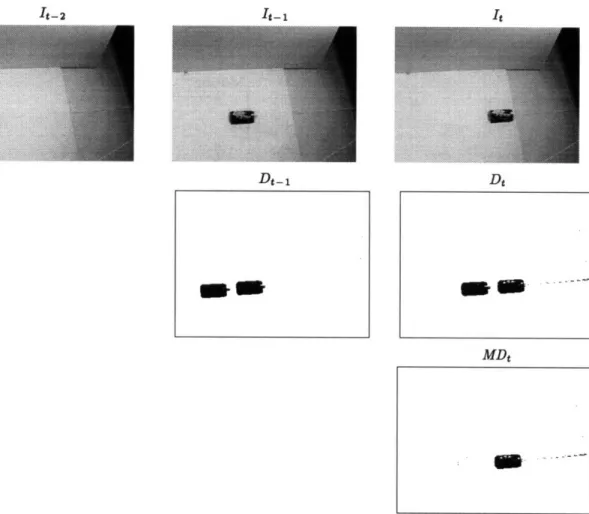
To compute the motion difference successive images are first subtracted and the absolute value thresholded to give a binary difference image indicating where significant change has occurred. More precisely,

.

j]

1 if l[i,

if [ijl - It-1 [i, j]l > 7 ,

(23)

0 otherwise.

Then, successive difference images are compared to give the binary motion difference image. This image consists of those pixels where there is change in the current difference but not in the previous difference:

MDt [i, j] 1 if Dt [i,j] = 1and Dt_[i, j] = 0,

MD [i, j] = (2.4)

0 otherwise.

Consider the can moving left to right in Figure 2-3. The corresponding difference images detect change at both the previous and new locations. However, the second difference, or motion difference image has almost entirely eliminated the response at the previous location while preserving the response at the new location.

The motion difference based prediction is computed from the first order moments of the motion difference image within two windows surrounding the previous feature location. The mean horizontal pixel index is computed within the horizontal window to give the estimated position i and the mean vertical pixel index is computed within the vertical window to give

I:

1 i'+WHw j*+Hw

NH

E E i MD[i,j] (2.5) i=i* -Www j=j*-Haw and i'+Wvw j*+Hvw 1= j .MD[i,j] (2.6) i=i*-Wvw j=j*-Hvw

where (i*, j*) is the previous detected location, NH and Nv are the number of motion difference pixels in the horizontal and vertical windows, and WHW, Wvw, HHW, and Hvw are the half widths and half heights of the horizontal and vertical windows.

An example of these windows on the can sequence is shown in Figure 2-4. The horizontal and vertical windows are shown centered on the previous patch location which is shown in light gray. The motion difference pixels are shown in black. The cross-hairs show the location of the predicted new location, which is very close to the true position shown by the small square patch.

(21)

experi-It-1i

Dt- 1

Figure 2-3: Motion difference computation. Top row: can moving left to right, center row: difference images, bottom row: motion difference.

Figure 2-4: Computation of prediction based on motion difference windows

21

MDt

I-2

(22)

Figure 2-5: Motion based tracker

ments.

The parameter values we have used for this algorithm are as follows: The search radius for the first prediction, SRI, is 2 and for the second (motion difference) prediction, SR2, is 8. The patch size is 11 x 11 (PR = 5). The horizontal window is 41 x 11 and the vertical window is 21 x 31

(HHW = 5, WHW = 20, Hvw = 15, Wvw = 10). All of these values are for 80 x 60 images and are

scaled linearly with image size. The image difference threshold, 7D, is 15 grey levels. These values of the parameters were found to give good results by Schneider and we have left them unchanged.

2.2 Motion Based Tracking Algorithm

The basic idea behind the second tracking method we will investigate is that the pixel locations in the image where there is motion can be grouped into connected regions corresponding to the objects we wish to track. The algorithm we will describe was developed by Satyajit Rao[19] in the summer of 1994 and is currently in use in the Intelligent Room for tracking single people at a time. Again, some minor modifications have been done to convert the algorithm to our platform, further instrument it, and investigate small variations.

A block diagram of this algorithm is shown in Figure 2-5. First the regions of the image where change has occurred since the previous image are identified. Optical flow is computed at these locations and the places where motion was detected are grouped into connected regions. Finally, these motion regions are put into correspondence with the previously detected regions.

(23)

the previous image It-_ to locate the pixels where significant change has taken place and focus the computation on these locations. These locations are most easily represented using a binary image where each pixel tells whether there was significant change in the corresponding location of the input image. This is identical to the difference image used for the motion difference based prediction in the correlation based feature tracker:

S

1 if It [i,

j]

- It-1[i,j]i > TD,

Dt[i,j ] =

t[ ] ]

(2.7)

0 otherwise.

Next, at each of the locations where there was significant change, eg. Dt [i, j] = 1, we compute the optical flow from the previous image to the current image. Optical flow gives a vector at each image pixel pointing to the location that pixel moves to in the next image. There are two common techniques for computing optical flow, those using correlation of small image patches between the two images and those using the constant brightness equation[8] on the spatial and time derivatives of image brightness. We use a correlation based algorithm similar to the feature point tracker described previously to get a dense set of correspondences between the previous and current images using small image patches. The matching is done using a sum of absolute differences (SAD) measure, similar to the SSD measure discussed previously. We denote by SAD(i, j, k, 1) the match score of the square patch of radius Rp centered at (i, j) in image It-1 with the patch centered at (k, 1) in image It:

Rp Rp

SAD(i,j,k,l) = E

E

IMt_[i

+

m,j

+

n]- It[k+m, + nil.

(2.8)

m=-Rp n=--Rp

The optical flow at a pixel (i, j) is computed as

J

arg min SAD(i, j, i + z, j + y) if min SAD(i, j, i + x, j + y) < TM, OF(i, j) -Rs<,y!Rs -Rs<:,y<Rs

(no-match) otherwise.

(2.9)

This is simply the displacement within a small search window of radius Rs at which the patch centered at (i, j) in Itl- best matches a patch in It. If the match score is not below the match threshold TM there is no good matching patch and the optical flow has the special value (no-match). Finally, we can group the pixels where motion was detected into connected motion regions cor-responding to moving objects. Given the optical flow values, we generate a binary image telling at each image pixel whether motion was detected there. We define the MOTION image:

MO

1 Dt[i,j] = 1 and OF(i,j) $ (no-match) and IIOF(i,j)ll > 0,

MOTION[i, j] -- (2.10)

0 otherwise.

(24)

which labels any two pixels in the MOTION image within a distance of Rcc using the same label. Given these regions, all that remains is to determine correspondences between the objects being tracked and the motion regions. Since this algorithm was designed for tracking a single person, it uses a simple rule: it chooses the component closest to the last position the person was detected as the new location. If no motion was detected the person is considered to have stayed in the same place. The output consists of the bounding box for the motion region being tracked. Note that unlike the feature point tracker, this algorithm is able to track the whole moving object, not just a point on that object.

Examples of the steps of this algorithm can be seen in Figure 2-5. Images (a) and (b) show two consecutive frames of a sequence in which a cereal box is moving right to left. The difference image is shown in (c) and (d) shows the MOTION image containing the pixels where motion was detected. It is the same as the difference image, except for some boundary pixels where the optical flow is not computed due to the edge of the image. In (e), the two connected regions of motion pixels detected are shown, one in black and one in grey. Finally, in (f), the region corresponding to the cereal box which is being tracked has been selected and a bounding box and cross hairs drawn. The other region corresponds to a thin string the box is hanging by.

This algorithm is somewhat similar to that described by Woodfill and Zabih in [25]. However, each uses the motion information from the optical flow differently. Woodfill and Zabih propagate model from frame to frame using the detected flow, which tends to accumulate large errors over time. Rao, on the other hand, simply uses the flow to detect where motion is taking place based on two frames and then groups these locations. There is no accumulation of errors over long image sequences.

The values of the parameters we have used are: The patch radius for the optical flow, Rp, is 1

(3 x 3 patch) and the search radius, Rs, is 3 (7 x 7 region). The connected component radius, Rcc,

is 4 pixels. The match threshold, rM, is 20 grey levels times the patch area in pixels. The difference threshold, rD, is 20 grey levels. The values for Rp, Rs, and Rcc given are for 80 x 60 images and scale linearly with image size.

As implemented, this algorithm uses only intensity information (grey images). It would be easy to extend both the differencing and optical flow steps to make use of multiple channels. The direction of the motion could also be used in the grouping stage to only group nearby pixels with the same motion direction, thereby possibly separating nearby moving objects better. We will not investigate how these changes would affect the performance of the algorithm.

(25)

c. d.

Figure 2-6: Motion based tracker example: a. previous image, b. current image, c. difference image,

d. detected motion locations, e. two connected motion regions, f. new tracked motion region and

bounding box

(26)

2.3 Hausdorff Distance Model Based Tracking Algorithm

The third and final algorithm we will be investigating is a shape based tracking system developed

by Huttenlocher, et al.[10] and described there in detail. The method is based on a shape similarity

metric, called the Hausdorff distance, applied to 2D image edge feature points. This metric has been shown to perform well in the presence of noise and partial occlusions and can be computed quickly[9]. It does not rely on establishing explicit correspondences between the image and model feature points but rather matches entire groups of edge points. The code we will be testing was obtained from the authors of [10]. Some work has been done to instrument it further and some minor modifications have been made.

The basic idea behind the algorithm is to match a 2D model of the shape of the object acquired from the previous image against the edges found in the current image, considering all possible locations. The best match location determines the position of the object in the new frame. Then, the model is updated to reflect the features matched in the current image. By exploiting the global shape of the object being tracked, the method should provide significant advantages over purely local methods when there is significant clutter in the environment, there are multiple moving objects, or there are large motions of the objects between frames. This is a major reason we have chosen this as one of our algorithms to test. We hope that the shape based approach will be able to distinguish between multiple people and solve the person constancy problem by matching the shapes of the people being tracked between frames.

The algorithm considers the change in the image of the object between frames to be composed of a 2D motion and a 2D shape change. This decomposition allows articulated or non-rigid objects to be tracked without requiring any model of the object's dynamics, so long as the shape change is small enough between frames that the shape matching metric does not fail. The shape matching will be based on the Hausdorff distance, which is inherently insensitive to small perturbations in the edge pixels comprising the shape of the object.

2.3.1 Comparing 2D Shapes Using the Hausdorff Distance

The Hausdorff distance measures the extent to which each point of a set A lies near some point in a set B and vice versa. It is defined as

H(A, B) = max(h(A, B), h(B, A)) (2.11) where

h(A, B) = max min Ila - b l (2.12) aEA bEB

(27)

Figure 2-7: Example showing the computation of the Hausdorff distances between two point sets

and I - I is some underlying norm measuring the distance between the points of A and B. For our purposes we will use the Euclidean or L2 norm. The function h(A, B) is called the directed Hausdorff distance from A to B. It identifies the point a E A which is furthest from any point in B and gives the distance from a to the closest point in B. In effect, it computes the distance from each point in

A to the closest point in B, ranks all these distances, and gives the maximal such distance. Hence,

if h(A, B) = d then each point of A is within a distance d of some point in B and there it at least one point in A which is exactly a distance d from the nearest point in B. Thus h(A, B) tells how well the points in A match those in B.

The Hausdorff distance is the maximum of h(A, B) and h(B, A) and therefore measures the mismatch between the two point sets. If this distance is small, all points in A must be near points in B and vice versa. Figure 2-7 shows two point sets and illustrates the computation of the directed Hausdorff distances between them. The set A is represented by hollow circles and the set B by filled circles. Arrows from each point indicate the closest point in the other set. Hence, h(A, B) is the length of the longest arrow from a hollow circle to a filled circle, and H(A, B) is the length of the longest arrow.

The Hausdorff distance measures the mismatch between two point sets at fixed positions with respect to each other. By computing the minimum distance over all possible relative positions of the point sets we can determine the best relative positioning and how well the sets match at that positioning. The positions we consider can in general be any group of transformations. Here we will

(28)

consider only the set of translations of one set with respect to the other. Thus, we can define

MT (A, B) = min H(A e t, B) (2.13) t

to be the minimum Hausdorff distance between A and B with respect to translation. In Figure 2-7,

H(A, B) may be large but MT (A, B) is small because there is a relative translation which makes

the two point sets nearly identical.

We can use the Hausdorff distance to look for an instance of a model in an image. We consider the set A to be the 'model' and the set B to be the 'image' because it is most natural to consider the model translating with respect to the image. An edge detector or some other point feature detector can be used to get a set of points corresponding to the features of the model and image from intensity values. We then look for translations t for which H(A E t, B) < 6. We consider these translations of the model with respect to the image where the mismatch is small to be instances of the model. Note that because the full image may contain more than just an instance of the model, when performing the reverse (image to model) match, h(B, A

E

t), only those points in A which lie beneath the outline of the translated model should be considered. The distance threshold 6 is set to account for noise in the edge detection process and to allow for small amounts of uncertainty in the model's expected appearance due to small amounts of rotation, scaling, shape change, etc.

One final modification to the Hausdorff distance is needed for this to work well in practice. The fact that the Hausdorff distance measures the most mismatched point makes it very sensitive to the presence of outlying points. In order to deal robustly with this situation and to allow the object of interest to be partly occluded, we introduce partial distances. In computing h(A, B), we ranked the distances of points in A to the nearest point in B and chose the maximum distance. If instead, we choose the Kth ranked value we get a partial distance for K of the q model points:

hK(A, B) =

Kth

A

min Ila - b

_bEB

(2.14)

where K tA denotes the Kth ranked value in the set of distances. Thus, if hK(A, B) = d then K of

the model points are within distance d of image points. This definition automatically selects the K best matching points of A. In general, we choose some fraction f and set K = [fqj. It is easy to

extend this idea to get a bidirectional partial distance, HKL(A, B).

Efficient rasterized algorithms have been developed for finding all translations of a model with respect to an image where the partial Hausdorff distance is below some threshold distance[9]. We will not go into the details of this here.

(29)

Figure 2-8: Hausdorff distance model based tracker

2.3.2 Model Based Tracking Using the Hausdorff Distance

A simplified block diagram for the model based tracker is shown in Figure 2-8. The fundamental part

of the algorithm consists of two basic steps: locating the object in the current frame, and updating the object model. The inputs take the form of the current image, It, and the previous object model,

Mt-1. A binary image representation is used, with the non-zero pixels representing sets of points.

For simplicity, the model is a rectangular sub-image consisting of a subset of the pixels found in the image at the location the object was found.

The current image, It, is actually a processed version of the intensity image input from the camera. A method similar to [5] is first used to extract intensity edges from the input intensity image. Next, any edge pixels corresponding to stationary background which appeared in the output of the edge detector for the previous image are removed. Finally, a shot noise filter is applied to remove any remaining stray background pixels, yielding edge image It.

Locating the object in the current image consists of using the forward Hausdorff distance to locate the best match location of the previous model, M-1, in the current image It. The forward distance measures the extent to which some portion of the model resembles the image, so minimizing this distance over all possible relative translations gives the best match location. This minimum value of the forward distance is given by

d = min hK(Mt-l

E

t, It)

and identifies the translation t* minimizing Equation 2.14. Note that all possible translations are considered, not just those within some local search window. At this position, at least K of the translated model points are within a distance d of image points. This match location t* is considered the new position of the object in the current frame and the bounding box of the model at that translation is output as the object's location.

(30)

the current image, trajectory information is used to disambiguate and determine the most likely match. Objects are assumed to continue in the same direction they have been moving. If there is no good match (e.g. d > bm where 6b is some match threshold), the tracker tries to locate a good match for a previous model, by searching a database of canonical models. The canonical models are a subset of the models Mo ... Mt-2 constructed by selecting the distinctive looking ones. A new

model Mt is added to the set of canonical models if it does not match any existing canonical model well, using the bidirectional Hausdorff distance HKL(A, B).

Once the object is located, the model Mt-1 is updated to build the new model Mt. The new model consists all edge pixels in It which are close (within a distance 6u) to points in the previous

model overlaid at the new object location, Mt-1

E

t* as follow:

Mt = {q

It I

minPEM,_t*

llP

-

ql < 6

}.

(2.15)

Finally, each border of the new model's bounding box is adjusted inward if there are relatively few non-zero pixels nearby or outward if there are a significant number of non-zero pixels nearby. Larger values of b6 allow the tracker to follow non-rigid motion better and to pick up new parts of the object that come into view. However, as br becomes larger it also becomes more likely that remaining background pixels will be incorporated into the model.

One final detail of the model update step is that we typically select at random a subset of the points given by Equation 2.15 for use as the new model Mt, instead of using every point selected by this equation. Given a model density factor aM, each point in Mt is selected with probability

aM to be included in a sparse model Mt, and the sparse model is used instead of the full model to

locate the object in the next image frame and to generate a new model in the next time step. A sparser model reduces the effect of background pixels getting included in the model and also speeds the computation. This detail is not described in [10] but was discovered through reading the code. The logic behind this aspect of the algorithm was confirmed by talking to the author of a second generation version of the tracker [3].

Figure 2-9 demonstrates the Hausdorff tracker in operation. The edge detector output is shown in (a) and the edge pixels which remain after the background is removed are shown in (b). The previous model Mt-1 is shown in (c). The updated model Mt is shown in (d). Finally, the model

Mt-1 is shown overlaid on image It demonstrating the match in (e).

The values of the parameters to this algorithm that we have used are those which were found to work well by the authors of [10]. Values for the major parameters of the algorithm are as follows: The match threshold b6 is 10 pixels. The forward fraction f is 0.8. The forward fraction determines the number of model pixels which must match well, K, in the Hausdorff distance equation. Recall that K = LfqJ, where q is the number of pixels in the model. The model update threshold by is 20

(31)

C.

Figure 2-9: Example of the Hausdorff tracker in operation. (a) shows the edge detector output, (b) shows the image It after removal of stationary background, (c) shows the previous model M-_1, (d) shows the new model Mt, and (e) shows the match of model M_-1 overlaid on image It.

31

C.

1 ·----

I

(32)

pixels. Finally, the model density factor am• is 0.10 unless otherwise specified. We will consider the effect of varying this parameter in the experiments.

(33)

Chapter 3 Experimental Design

Having described the algorithms we will be investigating, we will now proceed to discuss the design of the experiments we will be performing in order to analyze the strengths and weaknesses of these algorithms.

We are interested for now at least in designing a person tracking algorithm to observe the room through a single camera using a wide-angle lens. The camera will have a fixed position as well as fixed focus and focal length. Someday, we would like to incorporate multiple cameras for person tracking and may even want them to be actively computer controlled but for now we consider only this restricted case.

Since we have chosen to have the camera fixed, it is easy to do the analysis off-line. Because the algorithms will always get the same views and can do nothing to affect the images they receive, they can be fed pfilmed image sequences. This will greatly simplify testing because it enables re-peatability. The exact sequence can be re-run as many times as needed. The algorithm's parameters may be varied or the algorithms may be further instrumented to gain clearer insight into what is happening. Also, running the algorithms off-line allows us to relax the real-time constraint. We can step frame by frame for close analysis and are not required to find platforms capable of running the algorithms in real time, as long as we can run them at reasonable speeds. A disadvantage, however, is that we will be limited by the amount of data we can reasonably store; we will not be able to test on many hours of video.

In our experiments we will be using bounding boxes for the locations of the objects being tracked rather than some more precise representation such as the set of image pixels corresponding to the object. There are several reasons for this choice. First, we are only interested in a rough segmentation of the scene which will allow the higher level processes to focus their attention on those areas where the people are known to be. At this low level, it is not necessary to track the arms and hands precisely, for example. This will be left for the gesture recognition system, which will probably

(34)

only want to devote such computational resources to the single person who currently 'has the floor' and is commanding the room. Bounding boxes provide a very easy to manipulate and compact representation. They also make it easy to compare two segmentations. Finally, bounding boxes make it easy to hand segment the images for scoring the tracker output against the correct answer. Finally, we will be primarily looking at images sequences in which there is a single object to track. Some of the sequences do have small amounts of motion other than the primary object. None of the three algorithms are actually set up to simultaneously track multiple objects. They can be separately initialized to track each of a number of objects in the scene, however they have not been designed to deal with multiple objects in motion which can occlude each other. It is our primary goal to understand the features employed by each algorithm to understand how they might be modified and or combined to actually track multiple objects.

3.1 Image Sequences

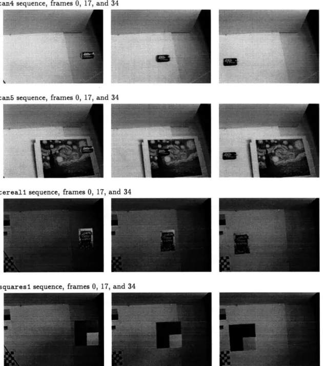
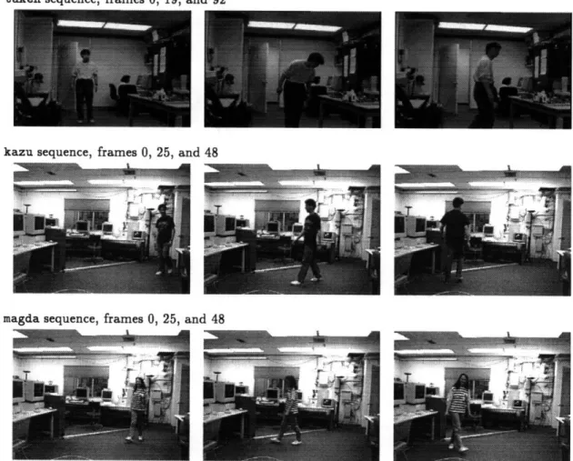
We now describe the seven video image sequences we will use for our testing. They have all been grabbed at half resolution in both the a and y dimensions. Due to hardware limitations, it was not possible to grab images at sufficient rates at full resolution and there would not have been sufficient storage either. The downsampling in the z dimension was done by sampling every even pixel of each row and the sampling in y was done by selecting even fields only. Selecting only the even fields was necessary to eliminate motion blur caused by the odd and even fields being captured 1/60th of a second apart. No smoothing was done prior to downsampling.

The sequences were mostly captured using the NTSC color input of an SGI Indy computer and stored as 24 bit RGB color images. The one exception is the takeh sequence which was captured using a VideoPix board in a Sun SparcSTATION 2 and stored as 8 bit grey-scale images. We unfortunately did not have access to a suitable 24 bit color frame grabber. The SGI captured images are 320 x 240 pixels and were taken using the NTSC color output of a Pulnix TMC-50 RGB CCD camera. The VideoPix captured images are 360 x 240 pixels and were taken from a Sanyo CCD grey-scale camera. Frame rates given below for both frame grabbers are approximate. For example, 7.5 frames per second means that for the most part every fourth even field was captured. However, paging of the computers virtual memory system and other effects cause frames to be missed occasionally.

The image sequences we will use for our testing fall into two classes. Four contain rigid objects undergoing a controlled motion. These motions were made with a computer controlled linear posi-tioner. The positioner was arranged horizontally on a table, and pulleys were used to route two thin threads from the moving platform to the stationary end of the positioner and up to the ceiling. The objects were hung such that they moved vertically as the positioner was controlled to move back

Design of a person tracking algorithm for the intelligent room

Design of a -Person Tracking Algorithm

for the Intelligent Room

by

Gregory Andrew Klanderman

Submitted to the Department of Electrical Engineering and Computer Science

in partial fulfillment of the requirements for the degree of

Master of Science in Computer Science and Engineering

at the

MASSACHUSETTS INSTITUTE OF TECHNOLOGY

August 1995

@

Massachusetts Institute of Technology 1995. All rights reserved.

Signature of Author

... . ...

.'...

Department of ilectrical Engineering and Computer Science

August 18, 1995

Certified by ... ...

--

•

.

...

W. Eric L. Grimson

Professor of Computer Science

Thesis Supervisor

(71,

Accepted by...

. . .

N.. :

V•e,...

F. R. Morgenthaler

Chairman, epartmental ommittee on Graduate Students

~nr

NOV

0

2

1995

Design of a Person Tracking Algorithm

for the Intelligent Room

by

Gregory Andrew Klanderman

Abstract

Acknowledgments

Contents

Chapter 1

Introduction

1.1

Person Tracking

1.2

Difficulty

1.3

Related Work

1.4

Approach

Chapter 2

Tracking Algorithms

2.1

Correlation Based Feature Tracking Algorithm

J

.

j]

1 if l[i,

if [ijl - It-1 [i, j]l > 7 ,

(23)

I:

NH

experi-It-1i

I-2

2.2

Motion Based Tracking Algorithm

S

j]

Dt[i,j ] =

(2.7)

SAD(i,j,k,l) = E

E

IMt_[i

+

m,j