Parafermionic theory with the symmetry Z_5

HAL Id: hal-00000101

https://hal.archives-ouvertes.fr/hal-00000101

Submitted on 13 Dec 2002

HAL is a multi-disciplinary open access

archive for the deposit and dissemination of sci-entific research documents, whether they are pub-lished or not. The documents may come from teaching and research institutions in France or abroad, or from public or private research centers.

L’archive ouverte pluridisciplinaire HAL, est destinée au dépôt et à la diffusion de documents scientifiques de niveau recherche, publiés ou non, émanant des établissements d’enseignement et de recherche français ou étrangers, des laboratoires publics ou privés.

Vladimir Dotsenko, Jesper Jacobsen, Raoul Santachiara

To cite this version:

Vladimir Dotsenko, Jesper Jacobsen, Raoul Santachiara. Parafermionic theory with the symmetry Z_5. Nuclear Physics B, Elsevier, 2003, pp.259. �hal-00000101�

ccsd-00000101 : 13 Dec 2002

Vladimir S. Dotsenko(1)_{, Jesper Lykke Jacobsen}(2) _{and Raoul Santachiara}(1)

(1) LPTHE1_{, Universit´e Pierre et Marie Curie, Paris VI}

Boˆıte 126, Tour 16, 1er _{´etage, 4 place Jussieu, F-75252 Paris Cedex 05, France.}

(2) Laboratoire de Physique Th´eorique et Mod`eles Statistiques, Universit´e Paris-Sud, Bˆatiment 100, F-91405 Orsay, France.

[email protected], [email protected], [email protected]

Abstract.

A parafermionic conformal theory with the symmetry Z5 is constructed, based on the

second solution of Fateev-Zamolodchikov for the corresponding parafermionic chiral algebra. The primary operators of the theory, which are the singlet, doublet 1, doublet 2, and disorder operators, are found to be accommodated by the weight lattice of the classical Lie algebra B2. The finite Kac tables for unitary theories are defined and the formula for the

conformal dimensions of primary operators is given.

1. Introduction

Extra discrete group symmetries in two-dimensional critical phenomena are naturally realised by parafermionic chiral algebras. The most well-known and widely used parafermionic conformal theory is due to Fateev and Zamolodchikov [1]. It describes, in particular, the self-dual fixed points of a particular lattice model with ZN symmetry [1,2].

In terms of the associativity constraint for physically consistent chiral algebras, the parafermions of the theory [1] represent the first solution, with the minimal possible values of the conformal dimensions (or spins) of the parafermionic currents. In this solution the central charge of the corresponding Virasoro algebra is a function of N only, i.e., for each N of the group ZN there is just one conformal theory, with a given, fixed value cN of the

central charge.

These same authors gave in the Appendix of Ref. [1] a second solution of the associative parafermionic chiral algebra, with the next allowed values of the spins of the parafermions.

In the second ZN symmetric solution the central charge remains a free parameter, for each

N .

The case N = 2 of this second solution corresponds to the superconformal theory. The

conformal theory corresponding to the second solution with Z3 symmetry has been fully

constructed by Fateev and Zamolodchikov in a subsequent work, Ref. [3]. It produces an infinite set of conformal theories which are selected by applying the degeneracy condition to the representations generated by physical fields, similar to the case of minimal models of purely conformal (non-extended) conformal field theory. This infinite set of conformal theories was supposed [3] to correspond to higher, multicritical fixed points of physical statistical systems with the symmetry Z3. And in fact, the first theory in this set (the one

with the least value of the central charge) was shown to correspond to the tricritical Potts model.

For the second associative solution of the chiral algebra [1], the conformal theories with N > 3 (i.e., with symmetries Z4, Z5, Z6 etc.) have not been constructed so far. The

purpose of our present work is to build the corresponding theories. In particular, we shall define the Kac formula giving the conformal dimensions of physical (primary) fields, which realise degenerate representations of the corresponding parafermionic chiral algebras.

The first of these theories, the one of N = 4, turns out to be trivial in the sense that it factorises into two independent superconformal chiral algebras, with fields of dimensions 2 and 3/2.

The first new theory is therefore that of Z5. This theory in itself turns out to be so

rich, and also representative for the whole class (whilst being the simplest at the same time), that it appeared reasonable for us to present it separately, in all the details. The present paper is therefore devoted to the theory Z5, and generalisations will be given in a

following work [4].

One extra result which we have used in our construction is that the central charge for the second solution of the ZN parafermionic algebra agrees with that of the coset [5]

SOk(N ) × SO2(N ) SOk+2(N ) , (1.1) which is c = (N − 1) µ 1 − N (N − 2)_{p(p + 2)} ¶ , (1.2) p = N − 2 + k. (1.3)

In the construction of the representation theory of the parafermionic algebra this observation turns out to be extremely useful.

Our paper is organised as follows. In Section 2 we review some technical details on the second associative solution of the chiral algebra as found in Ref. [1]. We then specialise

to the case of Z5. The structure of the representation modules of the various physical

operators (singlets, doublets, disorder operators) are fixed. We present explicit calculations of the first degeneracies in these modules. The resulting conformal dimensions, and the levels on which singular states are found, serve as initial conditions for dressing the entire theory. In Section 3 we give the Kac formula of the theory. We give the boundary terms corresponding to the various sectors of the theory.

The general question of determining the appropriate sector label for each operator in the theory is addressed in Section 4. We give a first argument, based on fusion rules and an assumed Coulomb gas construction. Some aspects of this argument are then verified by considering differential and characteristic equations for three-point functions. We also give the general formula for the eigenvalues of the parafermionic zero modes for the disorder operators. The conclusions are given in Section 5.

Four appendices deal with technical points of the calculations.

2. Parafermionic algebras in different sectors. First degeneracies

The operator product expansions of chiral fields within the second solution of the ZN

symmetric parafermionic algebra is given in Appendix A of Ref. [1]. They take the form

Ψq(z)Ψq0(z0) = λ q,q0 q+q0 (z − z0₎∆q+∆q0−∆q+q0 (2.1) × ½ Ψq+q0 (z0 ) + (z − z0₎∆q+q0 + ∆q− ∆q0 2∆q+q0 ∂z0Ψq+q 0 (z0_{) + . . .} ¾ , q + q0 6= 0 Ψq(z)Ψ−q(z0) = 1 (z − z0₎2∆q ½ 1 + (z − z0)22∆q c T (z 0 ) + . . . ¾ (2.2) Here the structure constants λq,q_q+q00 and the central charge c (of the Virasoro algebra) are

given by the expressions: (λq,q_q+q00)2 =

Γ(q + q0

+ 1)Γ(N − q + 1)Γ(N − q0_{+ 1)}

× Γ(q + q 0 + v)Γ(N + v − q)Γ(N + v − q0_)Γ(v) Γ(N + v − q − q0_{)Γ(q + v)Γ(q}0_{+ v)Γ(N + v)}, (2.3) c = 4(N − 1)(N + v − 1)v (N + 2v)(N + 2v − 2). (2.4)

The dimensions of the fields {Ψq

(z)} have the following form:

∆q = ∆N −q = 2q(N − q)

N . (2.5)

Note in particular that the field Ψ−q _{in (2.2) is assumed to have dimension ∆}

N −q, in the

sense that the indices q referring to the ZN charge are always defined modulo N . Thus,

ΨN −q

≡ Ψ−q

≡ (Ψq₎+_{, ∆}

N −q ≡ ∆−q. (2.6)

In the expressions (2.3)–(2.4) v is a free parameter, which was chosen in [1] to parametrise this solution. If one defines

v = 2k (2.7)

then the expression (2.4) for the central charge c could also be represented as in (1.2), making connection to the coset (1.1) [5].

From now on we specialise in this paper to the case N = 5, for the reasons given in the Introduction. In this case the Z5 charge q takes the values 0, ±1, ±2, and we have the

following parafermionic fields:

Ψ±1(z), Ψ±2(z). (2.8)

Together with the identity and the stress-energy operator T (z) these fields make a closed operator algebra, given by Eqs. (2.1)–(2.2). Their dimensions are

∆1 = 8 5, ∆2 = 12 5 (2.9) according to Eq. (2.5).

On the side of the representation fields, primary fields of the algebra (2.1)–(2.2), we should expect the singlet operators:

Φ0(z, ¯z) (q = 0) (2.10)

the doublet 1 operators:

Φ±1(z, ¯_{z) (q = ±1)} (2.11)

and the doublet 2 operators:

Φ±2(z, ¯_{z) (q = ±2).} (2.12)

In addition to these usual representations of the Z5 group we expect the spectrum to

include a quintuplet (5-plet) of Z2 disorder operators:

{Ra(z, ¯z), _{a = 1, 2, 3, 4, 5}.} (2.13)

The presence of disorder operators reflects the fact that the theory is, in fact, invariant under a larger group than Z5, viz. the dihedral group D5. This group includes, in addition

to Z5, also the Z2 reflections with respect to the five axes shown in Fig. 1.

This higher symmetry stems from the fact that in the solution (2.1)–(2.5) everything is symmetric with respect to the ZN charge conjugation:

q → N − q. (2.14)

(For the structure constants (λq,q_q+q00)2 in Eq. (2.3) the demonstration requires a little algebra

with products.)

The disorder fields have previously been shown to be in the spectrum of the Z3 theory,

second solution, as constructed in Ref. [3]. They appear as triplet representations in this case. The disorder fields also appear in the first solution [1] (for the case of general ZN),

One could object that the disorder fields {Ra(z, ¯z)} in Eq. (2.13) are on a somewhat

different footing than the standard (singlet and doublet) representation fields. Namely, the disorder fields complete the cyclic group Z5, as generated by 1 = Ψ0(z), Ψ±1(z) and Ψ±2(z),

to the dihedral group D5. However, there is a crucial difference between the Ψ and the R

fields. The first are chiral, or holomorphic, whilst the latter are non-chiral, like the rest of the representation operators. So despite of the fact that the symmetry of the theory is D5,

not all of the elements in the dihedral group are represented in the chiral algebra but only those of the biggest abelian subalgebra, Z5. The rest of the group elements find themselves

in the representation space, as disorder operators.

This is at least the structure of the present theory, and of the theory Z3 in Ref. [3].

Summarising, we expect that the representation space of the theory Z5 can be divided

into singlet, doublet 1, doublet 2, and disorder operators, cf. Eqs. (2.10)–(2.13).

It is already a standard point that the spectrum, for a given chiral algebra with a free parameter (the central charge (2.4), or the parameter v), is to be defined by the degeneracy condition of the representations. The reasoning why this is so can be given in various ways, for example by demanding the closure of the operator algebra of primary (physical) fields.

To define the spectrum of dimensions of singlets, doublets, and disorder operators, we have to define the representations of the chiral algebra in the corresponding sectors. One then constructs the modules induced by the various primary fields, and demands their degeneracy.

As usual, it will be sufficient to analyse directly the degeneracies on the first few levels in the modules. The physical operators defined in this way become the basic ones in the Kac table. Using these basic fields we shall be able, in the following Sections, to define the whole set, the Kac table and the formula for the dimensions.

2.1. Structure of the representation modules

The level structure of the modules induced by the singlets and by the two types of doublets can be defined as follows. We first place the chiral fields, i.e., the parafermions Ψ±1(z), Ψ±2(z) as well as the stress-energy operator T (z), in the module of identity. The levels of the various operators in this module correspond to their conformal dimensions:

∆±1 = 8/5 and ∆±2 = 12/5. This partially filled identity module is shown in Fig. 2.

To make apparent the crucial role played by the Z5 charge q, we depict the modules by

separating the various charge sectors horizontally.

Next, the level spacing within each charge sector (along a given vertical line on the figure) should be equal to 1, as the monodromy of the Ψ fields is abelian. This is so with respect to the identity operator, and, more generally, with respect to the singlet and doublet

operators forming the usual representations of the abelian group Z5. So we can complete

the levels in the identity module as shown in Fig. 3. The states below I and above Ψ±1_{, on}

levels 2/5, 3/5, 1, and 7/5 are actually empty. They will however become occupied when the identity operator I, placed at the summit of the module, is replaced by a more general singlet state, Φ0_.

We can now read off from Fig. 3 the level structure of the doublet 1 (with Φ±1 _at

the summit) and the doublet 2 (with Φ±2 _{at the summit) modules by inspecting their}

corresponding submodules in Fig. 3. For instance, for the doublet 1 we should consider the two states in Fig. 3 on level 3/5 as being at the summit, i.e., by imposing the levels above these states to be empty. Then, everything has to be shifted upwards by 3/5, putting these states at level 0. Proceeding in this way one obtains the level structure of the modules for a singlet, a doublet 1, and a doublet 2 operator, as shown in Figs. 4, 5 and 6. The consistency of these manipulations is ensured by the associativity of the algebra of Ψ fields.

1

3

5

2

4

Z

Z

Z

Z

Z

Fig. 1.— The action of the parafermionic current Ψk_{can be represented pictorially as a 2πk/5}

rotation of a pentagon. A quintuplet of disorder operators augments the cyclic symmetry to a dihedral one, each operator corresponding to the Z2 reflection with respect to an axis

passing through one of the vertices of the pentagon. The labeling of the five axes, as shown on the figure, is also used to label the corresponding disorder operators.

I(z)

Fig. 2.— The position of the parafermionic currents in the identity module. The horizontal

axis shows the Z5 charge q. The vertical axis gives the level of a given state, here with

I(z)

Fig. 3.— Completion of the identity module. Each state is shown as a filled circle.

q=−2

q=−1

q=1

q=2

0

1

7/5

2/5

3/5

0

Φ

Fig. 4.— Representation module of a singlet operator. Arrows depict (some of) the possible

actions by the parafermionic mode operators (with an appropriate change of the Z5 charge

Φ

−1

q=−2

q=2

0

1

7/5

2/5

Φ

+1

4/5

q=0

Fig. 5.— Representation module of a doublet of operators of charge q = ±1, henceforth referred to as doublet 1. Note the existence of a zero mode linking the two states at the summit of the diagram.

0

1

q=0

Φ

−2

Φ

+2

q=1

q=−1

1/5

3/5

6/5

Fig. 6.— Representation module of a doublet 2 operator. The two states at the summit are linked by a zero mode.

developments of the chiral fields Ψ in the basis of the representation fields, Φ0_{, Φ}±1 _and

Φ±2_{, should be of the forms given below.}

In the singlet basis one has:

Ψ±1(z)Φ0(0) = X n 1 (z)∆1−3₅+nA ±1 −3₅+nΦ 0_(0), A±1₋3 5+nΦ 0_{(0) = 0, n > 0 (2.15)} Ψ±2(z)Φ0(0) = X n 1 (z)∆2−2₅+nA ±2 −2₅+nΦ 0_(0), A±2₋2 5+n Φ0(0) = 0, n > 0. (2.16)

The fact that positive-index mode operators annihilate Ψ0_{(0) is the usual highest-weight}

condition, expressing the fact that we are trying to make the representation fields primary with respect to the chiral algebra. Conversely, one gets:

A±1₋3 5+n Φ0(0) = 1 2πi I C0 dz (z)∆1−3₅+n−1_Ψ±1_(z)Φ0_{(0), (2.17)} A±2₋2 5+n Φ0(0) = 1 2πi I C0 dz (z)∆2−2₅+n−1_Ψ±2_(z)Φ0_{(0). (2.18)}

The arrows in Figs. 4–6 represent the actions of the mode operators A±1

µ and A±2µ . For the

sake of clarity not all possible arrows are shown. In particular, we do not show the upwards arrows which would represent the action on a descendent state. The “gaps” in the modules, i.e., the level of the first descendents, show up in the fractional shifts of the indices of the operators A±1

µ and A±2µ (e.g., µ = −3/5 + n in Eq. (2.17), etc.).

In a similar way, for the doublet 1 one gets:

Ψ±1(z)Φ∓1(0) = X n 1 (z)∆1−2₅+nA ±1 −2₅+nΦ ∓1_{(0), (2.19)} Ψ±1(z)Φ±1(0) = X n 1 (z)∆1−4₅+nA ±1 −4₅+nΦ ±1_{(0), (2.20)} Ψ±2(z)Φ∓1(0) = X n 1 (z)∆2+nA ±2 n Φ∓1(0), (2.21)

Ψ±2(z)Φ±1(0) = X n 1 (z)∆2−4₅+nA ±2 −4₅+nΦ ±1_{(0). (2.22)}

We remark that the action of Ψ±2(z) on Φ∓1(0) in Eq. (2.21) involves a zero mode A±20 ,

which acts between the states Φ±1_{(0) at the summit:}

A∓2₀ Φ±1(0) = h2,1Φ∓1(0). (2.23)

The index of the eigenvalue h2,1 refers to the indices of A and Φ. Another zero mode

appears in the action of Ψ±1_{(z) on Φ}±2_(0):

A±1₀ Φ±2(0) = h1,2Φ∓2(0). (2.24)

(The corresponding expansion, in the basis of Φ±2_{(0), is given below.) The eigenvalues}

h in Eqs. (2.23)–(2.24) characterise the representations, in addition to the values of the conformal dimensions of the fields Φ±1_{, Φ}±2 _{(which are the eigenvalues of the Virasoro zero}

mode L0).

The relations which are the inverse of Eqs. (2.19)–(2.22) read: A±1₋2 5+n Φ∓1(0) = 1 2πi I C0 dz (z)∆1−3₅+n−1_Ψ±1_(z)Φ∓1_{(0), (2.25)} A±1₋4 5+n Φ±1(0) = 1 2πi I C0 dz (z)∆1−4₅+n−1_Ψ±1_(z)Φ±1_{(0), (2.26)} A±2n Φ∓1(0) = 1 2πi I C0 dz (z)∆2+n−1_Ψ±2_(z)Φ∓1_{(0), (2.27)} A±2₋4 5+n Φ±1(0) = 1 2πi I C0 dz (z)∆2−4₅+n−1_Ψ±2_(z)Φ±1_{(0). (2.28)}

Finally, for the doublet 2 one gets the expansions:

Ψ±1(z)Φ∓2(0) = X n 1 (z)∆1−1₅+nA ±1 −1₅+nΦ ∓2_{(0), (2.29)} Ψ±1(z)Φ±2(0) = X n 1 (z)∆1+nA ±1 n Φ±2(0), (2.30)

Ψ±2(z)Φ∓2(0) = X n 1 (z)∆2−3₅+nA ±2 −3₅+nΦ ∓2_{(0), (2.31)} Ψ±2(z)Φ±2(0) = X n 1 (z)∆2−1₅+nA ±2 −1₅+nΦ ±2_{(0), (2.32)}

the inverse relations being: A±1₋1 5+n Φ∓2(0) = 1 2πi I C0 dz (z)∆1−1₅+n−1_Ψ±1_(z)Φ∓2_{(0), (2.33)} A±1_n Φ±2(0) = 1 2πi I C0 dz (z)∆1+n−1_Ψ±1_(z)Φ±2_{(0), (2.34)} A±2₋3 5+n Φ∓2(0) = 1 2πi I C0 dz (z)∆2−3₅+n−1_Ψ±2_(z)Φ∓2_{(0), (2.35)} A±2₋1 5+nΦ ±2_{(0) =} 1 2πi I C0 dz (z)∆2−1₅+n−1_Ψ±2_(z)Φ±2_{(0). (2.36)}

2.2. Degeneracy of the modules

Having defined the mode operators, A±1

µ and A±2µ , we now turn to the problem of

degeneracies in the modules.

To analyse the degeneracies, we shall need to compute various matrix elements of the mode operators. To this end, we shall make extensive use of the commutation relations of the mode operators, in the various sectors. For convenience, we have listed the complete set of commutation relations in Appendix A: these are all obtained in a way analogous to that used in Refs. [1,3]. We also exemplify in Appendix A the computation of some of the matrix elements needed in the subsequent analysis.

2.2.1. Doublet 1

For the doublet 1 module, depicted on Fig. 5, we begin by imposing degeneracy at level

2/5. Forming the linear combination2

χ0₋2 5 = aA 1 −2₅Φ −1_{+ bA}−1 −2₅Φ 1_{, (2.37)}

we wish to make it into a primary operator, i.e., to ensure that it is annihilated upon action by positive index mode operators. In this case it will be sufficient to verify that

A1₊2 5χ 0 −2₅ = 0 and A −1 +2 5χ 0 −2₅ = 0. (2.38)

The others arrows going upwards in Fig. 5 will be zero for trivial reasons. The conditions (2.38) for the state (2.37) can be rewritten as:

aA12 5A 1 −2₅Φ −1_{+ bA}1 2 5A −1 −2₅Φ 1 _{= 0,} aA−12 5 A1₋2 5Φ −1_{+ bA}−1 2 5 A−1₋2 5 Φ1 = 0, (2.39) where, obviously, A1 2 5 A1 −2₅Φ

−1 _{∝ Φ}1 _{etc. It is convenient to define matrix elements µ by}

A12 5A 1 −2₅Φ −1 _{= µ}(1,1;−1) 2 5,−25 Φ 1_{, (2.40)} A12 5A −1 −2₅Φ 1 _{= µ}(1,−1;1) 2 5,−25 Φ 1_{, (2.41)} A−12 5 A1₋2 5Φ −1 _{= µ}(−1,1;−1) 2 5,− 2 5 Φ−1, (2.42) A−12 5 A−1₋2 5 Φ1 = µ(−1,−1;1)2 5,− 2 5 Φ−1. (2.43)

By the Z2 reflection symmetry (q ↔ −q) we have

µ(1,1;−1) = µ(−1,−1;1), (2.44) µ(1,−1;1) = µ(−1,1;−1). (2.45)

2_{We adopt the convention of denoting singular vectors as χ}q

−µ, where q denotes the Z5

To compute the remaining two matrix elements in Eq. (2.39) we need the commutation relations of the mode operators A±1

µ . In Appendix A it is shown that

µ(1,1;−1)2 5,− 2 5 = λ1,1₂ h2,1, (2.46) µ(1,−1;1)2 5,− 2 5 = − 2 25+ 2∆1 c ∆Φ1. (2.47)

Here, λ1,1₂ is one of the structure constants (2.3) of the chiral algebra (2.1) and h2,1 is the

eigenvalue of Φ∓1 _{with respect to the zero mode A}±2_{, as defined in Eq. (2.23). Finally,}

∆1 = 8/5 is the dimension of Ψ±1, and ∆Φ1 is the as yet unknown dimension of the operator

Φ±1_.

A non-trivial solution of the system (2.39) exists provided that ¯ ¯ ¯ ¯ ¯ ¯ µ(1,1;−1) _µ(1,−1;1) µ(−1,1;−1) _µ(−1,−1,1) ¯ ¯ ¯ ¯ ¯ ¯ = 0, (2.48)

from which one obtains:

¡λ1,1 2 h2,1 ¢2 = µ −₂₅2 + 2 5c∆Φ1 ¶2 . (2.49)

We recall that, for a given operator Φ1 _{or Φ}−1_{, we need to determine both the eigenvalue}

h2,1 and the dimension ∆Φ1. By imposing degeneracy at level 2/5, we have obtained

Eq. (2.49), which defines h2,1 as a function of ∆Φ1 and c. (Note also that the structure

constant λ1,1₂ is a function of c, by Eqs. (2.3)–(2.4).)

In conclusion, degeneracy at level 2/5 is not sufficient to define also ∆Φ1 (as a function

of c). We have two unknowns, h2,1 and ∆Φ1. So we need one more constraint, in addition

to that in Eq. (2.49).

We shall therefore require that the doublet 1 module be degenerate also at level 4/5. This is obtained by demanding the degeneracy of the state

χ2₋4 5 = ˜aA 1 −4₅Φ 1_{+ ˜bA}−2 −4₅Φ −1_{. (2.50)}

The reason for considering a linear combination of two states only is that the “indirect” descendent at level 4/5, obtained by descending through the state which remains at level 2/5 after imposing the degeneracy constraint at that level, is linearly dependent on the direct descendents. More precisely, by using the mode operator algebra given in Appendix A, one finds (in Appendix A) that

A2₋2 5A 1 −2₅Φ −1 _{= A}2 −2₅A −1 −2₅Φ 1 _(2.51)

is linearly dependent on the states A1₋4 5Φ 1 _{and A}−2 4 5 Φ −1_{. (2.52)}

(In Eq. (2.51) we have used the linear dependence resulting from the degeneracy at level 2/5.)

The degeneracy of the state (2.50) takes the form ¯ ¯ ¯ ¯ ¯ ¯ ¯ µ(−1,1;1)4 5,−45 µ (−1,−2;−1) 4 5,−45 µ(2,1;1)4 5,− 4 5 µ(2,−2,−1)4 5,− 4 5 ¯ ¯ ¯ ¯ ¯ ¯ ¯ = 0, (2.53)

involving the following matrix elements (see Appendix A for details): A−14 5 A1₋4 5Φ 1 ₌ µ 3 25+ 2∆1 c ∆Φ1 ¶ Φ1 _{≡ µ}(−1,1;1)4 5,− 4 5 Φ1, (2.54) A−14 5 A2₋4 5Φ 1 _{= λ}21 −2h2,1Φ1 ≡ µ(−1,−2;−1)4 5,− 4 5 Φ1, (2.55) A24 5A 1 −4₅Φ 1 _{= λ}21 −2h2,1Φ1 ≡ µ(−2,1;1)4 5,− 4 5 Φ1, (2.56) A24 5A −2 −4₅Φ 1 ₌ µ 4 (λ1,1₂ )2 · 4 5y 2 − 2∆_c1(∆Φ1 +2 5)y ¸ + 9 5(λ1,1₂ )2y 2₊ 3 2y ¶ Φ−1 ≡ µ(2,−2;−1)4 5,− 4 5 Φ−1, (2.57) where y = λ1,1₂ h2,1= − 2 25+ 2∆1 c ∆Φ1. (2.58)

The solutions of Eq. (2.53), with the ingredients (2.54)–(2.57) as well as Eq. (2.49), have a rather simple form, in spite of its appearances. They can be presented as:

∆(1)_Φ1 = 3 5 p + 5 p , ∆ (2) Φ1 = 3 5 p − 3 p + 2, (2.59) ∆(3)_Φ1 = 1 10 p2_{+ 2p − 15} p(p + 2) , (2.60)

where the parameter p has been defined in Eq. (1.3). For N = 5,

p = 3 + k = 3 + v

2 (2.61)

where v is the parameter in the solution (2.1)-(2.5) of the chiral algebra; we recall from Eq. (2.7) that v = 2k.

By introducing the parameters

α2₊ = p + 2 p , α 2 −= p p + 2 (2.62)

which are suggestive from the formula for the central charge (1.2), the solutions for the dimensions in Eqs. (2.59)–(2.61) take the form

∆(1)_Φ1 = 3 2α 2 +− 9 10, ∆ (2) Φ1 = 3 2α 2 −− 9 10, (2.63) ∆(3)_Φ1 = − 3 8(α 2 ++ α2−) + 17 20. (2.64)

We shall defer to the next section further discussion on the significance of the solutions (2.63)–(2.64).

We state once again that in the Z5 theory the modules have to be doubly degenerate,

on two levels simultaneously, to reach the goal that the dimension of the primary field gets fixed as a function of c.

2.2.2. Doublet 2

The module of Φ±2_{, shown in Fig. 6, has its first descendents at level 1/5, with q = ±1.}

We could consider one side, q = −1 for instance, because what is constructed for q = −1 will also be confirmed by the algebra for q = +1, due to the Z2 reflection symmetry.

At level 1/5 it would appear that there are two states: A1₋1

5Φ

−2 _{and A}2

−1₅Φ

2_{. (2.65)}

However, it turns out that they are proportional to one another. Indeed, by the commutation relation {Ψ1_{, Ψ}1_}Φ2 _{(see Appendix A) with n = m = 0, one gets:}

λ1,1₂ A2₋1 5Φ 2 _{= 2A}1 −1₅A 1 0Φ2 = 2A1−1₅h1,2Φ −2_{, (2.66)} λ1,1₂ A2₋1 5Φ 2 _{= 2h} 1,2A1₋1 5Φ −2_{, (2.67)}

where the number h1,2 is the zero mode eigenvalue, yet to be fixed.

With this simplification, in order to have a degeneracy at level 1/5, it suffices to require that the state

χ−1₋1 5 = A

1 −1₅Φ

−2 _(2.68)

be primary. Also, it is sufficient to require that it be annihilated by A−1₊1 5

only, and not by both A−1₊1

5 and A

2

+1₅. The algebraic reason for this follows from a relation analogous to

Eq. (2.67), but for positive index mode operators. We therefore require that

A−11 5

A1₋1 5Φ

−2 _{= 0, (2.69)}

and by means of the commutation relation {Ψ1_{, Ψ}−1_}Φ−2 _{with n = m = 0}

³ A1₀A−1₀ + A−11 5 A1₋1 5 ´ Φ−2 = µ − 3 25+ 2∆1 c ∆Φ2 ¶ Φ−2 (2.70)

this takes the form (h1,2)2 = − 3 25 + 2∆1 c ∆Φ2. (2.71)

If we impose the condition (2.71), the state (2.68) can be put equal to zero, thus reducing the module. As a consequence of the proportionality (2.67) the second state in Eq. (2.65) will then also vanish. Thus, after this reduction, level 1/5 will be completely degenerate, or empty.

Analogous to the case of doublet 1, the constraint (2.71) only defines (h1,2)2 as a

function of ∆Φ2 and c. We therefore turn to level 3/5.

By the commutation relation {Ψ1_{, Ψ}1_}Φ−2 _{with n = m = 0 we have}

2A1₋2 5A 1 −1₅Φ −2 _{= λ}1,1 2 A2−3₅Φ −2_{. (2.72)} Since now A1 −1₅Φ

−2 _{= 0, by the previous degeneracy, one obtains}

A2₋3 5Φ −2 _{= 0. (2.73)} Similarly, because of A−1₋1 5 Φ2 _{= 0, one gets} A−2₋3 5Φ 2 _{= 0. (2.74)}

In conclusion, the complete degeneracy at level 1/5 implies that, after the reduction consisting in factoring out the degenerate submodule, level 3/5 is also empty.

To fix ∆Φ2 we therefore go on to examine the next available level, which is level 1. It is

not difficult to verify that at level 1 we have to consider the state

χ−2₋₁ = aL−1Φ−2+ bA1−1Φ2 (2.75)

and require the following degeneracy conditions to be satisfied:

In terms of the matrix elements µij defined by

L1L−1Φ−2 = µ11Φ−2, (2.77)

L1A1−1Φ2 = µ12Φ−2, (2.78)

A−1₁ L−1Φ−2 = µ21Φ2, (2.79)

A−1₁ A1₋₁Φ2 = µ22Φ2, (2.80)

the degeneracy criterion reads

µ11µ22− µ12µ21= 0. (2.81)

Using the Virasoro algebra and the commutation relations {Ψ1_{, Ψ}−1_}Φ−2 _{and {T, Ψ}Φ the}

required matrix elements are readily computed:

µ11 = 2∆Φ2, (2.82) µ12 = 8 5h1,2, (2.83) µ21 = 8 5h1,2, (2.84) µ22 = 1 5(h1,2) 2₊ 7 25 + 2∆1 c ∆Φ2, (2.85)

and the resulting criterion is 2∆Φ2µ 1 5(h1,2) 2₊ 7 25+ 2∆1c∆Φ2 ¶ −64₂₅(h1,2)2 = 0. (2.86)

Solving Eqs. (2.71) and (2.86) one gets the following solutions: ∆(1)_Φ2 = α2₊− 3 5, ∆ (2) Φ2 = α2−− 3 5 (2.87) with α2 ± defined in Eq. (2.62). 2.2.3. Singlet

For the singlet module, depicted in Fig. 4, the first descendents are at level 2/5 in the sector q = ±2. By charge conjugation symmetry it is sufficient to consider one of them.

One may thus define the state χ2₋2 5 = A 2 −2₅Φ 0_{, (2.88)}

subject to the constraint

A−22 5

χ2₋2

5 = 0. (2.89)

Using the commutation relation {Ψ2_{, Ψ}−2_}Φ0 _{given in Appendix A, with m = −1, n = 0,}

one obtains: ³ A27 5A −2 −7₅ + A −2 2 5 A2₋2 5 ´ Φ0 = 2∆2 c ∆Φ0Φ 0_{. (2.90)}

We observe that the constraint (2.89) has the consequence of fixing a matrix element at a lower level: A2 7 5A −2 −7₅Φ 0 ₌ 2∆2 c ∆Φ0Φ 0_{. (2.91)}

Accepting Eqs. (2.89) and (2.91) we can eliminate the only state on level 2/5. We thus put A2₋2

5Φ

0 _{= 0. (2.92)}

We next demand degeneracy at level 3/5 in the sector q = ±1. Once the level 2/5 is

empty, there will be only a single state on level 3/5, up to the Z2 symmetry q ↔ −q. We

therefore set χ1₋3 5 = A 1 −3₅Φ 0_{, (2.93)}

subject to the constraint

A−13 5

χ1₋3

5 = 0. (2.94)

Using the commutation relation {Ψ−1_{, Ψ}1_}Φ0 _{in Appendix A, with n = 1, m = 0, one}

obtains: A13 5A −1 −3₅Φ 0 ₌ 2∆1 c ∆Φ0Φ 0_{. (2.95)}

The constraint (2.94) requires that

∆Φ0 = 0. (2.96)

2.3. Sector of the disorder operator Ra

2.3.1. Structure of the disorder modules

The disorder operator (quintuplet) Ra(z, ¯z), a = 1, 2, 3, 4, 5, has non-abelian monodromy

with respect to the chiral fields Ψ±1_{(z), Ψ}±2_{(z). This amounts to the decomposition of the}

local products Ψ+1_(z)R

a(0) and Ψ+2(z)Ra(0) into half-integer powers of z:

Ψ+1(z)Ra(0) = X n 1 (z)∆1+n₂ A 1 n 2Ra(0), (2.97) Ψ+2(z)Ra(0) = X n 1 (z)∆2+n₂ A 2 n 2Ra(0). (2.98)

Because of the non-abelian monodromy of the disorder fields, the expansion of the products Ψ−1_(z)R

a(0) and Ψ−2(z)Ra(0) are related to those in Eqs. (2.97)–(2.98), by an analytic

continuation of z around 0 on both sides of these two equations. One finds: Ψ−1(z)Ra(0) = X n (−1)n (z)∆1+n₂A 1 n 2 U_{Ra(0), (2.99)} Ψ−2(z)Ra(0) = X n (−1)n (z)∆2+n₂A 2 n 2 (U) 2_R a(0). (2.100)

Here U is a 5 × 5 matrix which rotates the index of the disorder field backwards by one

unit: URa(0) = Ra−1(0). (Note that in Eq. (2.100) we have denoted the square of U by

(U)2 _{rather than by U}2_{. This notation is intended to avoid confusion with upper indices of}

operators which are abundant in our presentation.)

The theory of disorder operators has been fully developed in Ref. [6] in the context of the first parafermionic conformal field theory (with symmetry ZN), and in Ref. [3] in

the context of the second parafermionic theory (with symmetry Z3). As far as the general

properties (products, analytic continuations) of the disorder sector operators are concerned, the approach of Refs. [3,6] generalises directly to the present case. In Appendix B we present some details of the disorder sector which are specific to the second Z5 theory (the

one treated in this paper). In particular, the developments (2.97)–(2.100) are justified and

the commutation relations of the mode operators A1

n

2 and A

2

n

2 in the disorder sector are also

given.

As compared to Figs. 4–6, the level structure of the modules of disorder operators is relatively simple. There are only integer and half-integer levels, and there exists zero modes for all the operators {Ψq_{} acting on the quintuplet of disorder operators. For the zero}

modes one should have, in general:

A1₀Ra = h1(U)2Ra, (2.101)

A20Ra = h2(U)−1Ra. (2.102)

The matrices (U)2 _{and (U)}−1 _{turn the indices in accordance with the multiplication rules}

of Z5: we refer to Appendix B for details. The constants h1 and h2 are the eigenvalues of

Ra with respect to A10 and A20. As in the case of the doublets, these eigenvalues furnish

an additional characterisation of the disorder representations, in addition to the conformal dimension of Ra. Actually, it suffices to specify one of the eigenvalues, h1 or h2, since the

two are generally related, irrespective of the details of the representation of a particular

operator Ra. This can be seen by applying the commutation relation (B25) with n = m = 0.

We obtain 2A1 0A10Ra(0) = λ1,12 2∆2−3A20Ra(0) + 2−∆2−2 µ κ(0) + 16∆1 c ∆R ¶ (U)−1_R a(0), (2.103)

where κ(n) is defined in Eq. (B26). In particular, κ(0) = −11/10. Taking into account Eqs. (2.101)–(2.102) one obtains

2(h1)2 = λ1,12 2∆2−3h2+ 2−∆2−2 µ κ(0) + 16∆1 c ∆R ¶ . (2.104)

2.3.2. Degeneracy of the disorder modules

As discussed above, the modules of the disorder operators consist of integer and half-integer levels. The first descendents of a given primary operator Ra will therefore be

found at level 1/2. For a given value of the index a, there exist two states: ¡χ(1) a ¢ −1₂ ≡ A 1 −1₂(U) −2_R a= (U)−2A11 2Ra, (2.105) ¡χ(2) a ¢ −1₂ ≡ A 2 −1₂URa = UA 2 1 2Ra. (2.106)

The matrices (U)−2 _{and U commute with the action of the mode operators, A}1

−1₂ and A 2 −1₂.

They just compensate for the rotation of indices of the Ra which are produced by the action

of A1

−1₂ and A 2 −1₂.

In analogy with the computations for the doublet 1 operator (see above), one could now try to produce one primary state at level 1/2, by making a linear combination of the states (2.105)–(2.106). We shall, however, not follow this route. Instead, we shall require in this case that both states, (2.105) and (2.106), be primaries. Thus, the two of them will be eliminated eventually, and there will be a complete degeneracy at level 1/2.

It should be remarked that in this process of looking for degeneracies at the lowest levels in the modules there is a certain choice, and the way of performing the computations is not uniquely defined from the outset. For some of the choices, the solutions found (and the formulae for the dimensions in particular) will have to be classified as non-physical, not matching with the theory that we are constructing. In general, the number of possible solutions is bigger then the number of physical operators to be determined, and there is some redundancy. For instance, in the case of the doublet 1 module, if we had required that both states at level 2/5 be primaries, we would have found a non-physical value for the conformal dimension of the doublet, a value which would have to be discarded. Also, among the three solutions that we eventually found for the case of doublet 1, see Eqs. (2.63)–(2.64),

the first two will turn out to be physical whilst the third one is not.

The distinction between physical and non-physical solutions shall be done in the next section. All the solutions that we are getting at present will serve in the next section to fix the form of the Kac formula for dimensions and to fill the Kac table, positioning the singlets, doublets and disorder operators correctly. In this analysis some of the present solutions for ∆ will turn out to be inconsistent and will have be discarded.

Going back to the disorder operator Ra, the reason that we have decided to annihilate

both states at level 1/2, Eqs. (2.105) and (2.106), is that this yields physical solutions, consistent with the eventual Kac formula. So in this particular case, the two states which must be required to be degenerate in order to fix both h and ∆ are situated on the same level. This is not so in general. But for the fundamental disorder operator, with the two required degeneracies situated at the first descendent levels, these levels are both equal to 1/2.

In accordance with these remarks, we shall require that A11 2 ¡χ (1) a ¢ −1₂ = 0, A 2 1 2 ¡χ (1) a ¢ −1₂ = 0, (2.107) A11 2 ¡χ (2) a ¢ −1₂ = 0, A 2 1 2 ¡χ (2) a ¢ −1₂ = 0. (2.108) This gives: A11 2A 1 −1₂Ra= 0, A 2 1 2A 1 −1₂Ra = 0, (2.109) A11 2A 2 −1₂Ra= 0, A 2 1 2A 2 −1₂Ra = 0. (2.110)

From the algebra (B25), with n = 1, m = −1, one then obtains: µ A11 2A 1 −1₂ + 2 5A 1 0A10 ¶ Ra = λ1,12 2∆2−3A20Ra− 2−∆2−2 µ κ(1) + 16∆1 c ∆R ¶ (U)−1Ra. (2.111)

Imposing now that A1

+1 2A

1

−1₂Ra= 0, and replacing A 1

Eqs. (2.101)–(2.102), we find the relation 2 5(h1) 2 _{= λ}1,1 2 2∆2−3h2− 2−∆2−2 µ κ(1) + 16∆1 c ∆R ¶ . (2.112)

Here κ(1) = −1/10, from Eq. (B26).

Next, using the commutation relation (B28), first with n = 1, m = −1 and then with n = −1, m = 1, it is found that A11 2A 2 −1₂Ra= A 2 1 2A 1 −1₂Ra = µ −4 5h1h2+ 2 ∆2−∆1−2_λ2,1 −2h2− 2∆1−∆2−2λ−2,1−1 h1 ¶ U_{Ra. (2.113)} Using again Eqs. (2.109)–(2.110), this gives a second relation:

−4

5h1h2+ 2

∆2−∆1−2_λ21

−2h2− 2∆1−∆2−2λ−2,1−1 h1 = 0. (2.114)

Finally, combining the commutation relations (B25) and (B28), after some algebra it is found that A21 2A 2 −1₂Ra = 2−∆2+3 λ1,1₋₂ ·µ −4₅h2 + 1 4(2) ∆1−∆2−2_λ2,1 −1 ¶ A11 2A 1 −1₂(U) −1_R a + µ 12 5h1− 1 3(2) ∆2−∆1−2_λ2,1 −2 ¶ A11 2A 2 −1₂(U) 2_R a ¸ . (2.115)

As a result, if the matrix elements A1

1 2A 1 −1₂Ra and A 1 1 2A 2

−1₂Ra vanish, in this case all the

matrix elements in Eqs. (2.109)–(2.110) will vanish, as required.

Let us summarise the situation. The constraints expressing the complete degeneracy at level 1/2 in the module of a disorder operator Ra are given by Eqs. (2.112) and (2.114). In

addition, the zero mode eigenvalues h1 and h2 are related by Eq. (2.104). This set of three

equations allows us to express h1, h2 and ∆R as functions of c, or as functions of the related

parameters, p or α2

+, α2− defined in Eqs. (2.61)–(2.62).

Solving Eqs. (2.104), (2.112) and (2.114) one finds the following solutions for the conformal dimension ∆R: ∆(1)R = 1 4 p + 5 p , ∆ (2) R = 1 4 p − 3 p + 2, (2.116)

∆(3)R = 1 4 p2_{+ 2p − 5} p(p + 2) . (2.117) Expressed in terms of α2

+ = (p + 2)/p and α2− = p/(p + 2), these solutions take the form:

∆(1)_R = 5 8α 2 +− 3 8, ∆ (2) R = 5 8α 2 −− 3 8, (2.118) ∆(3)_{R = −} 5 16(α 2 ++ α2−) + 7 8. (2.119) 3. Kac formula

In Eq. (1.1) it was observed [5] that the central charge of the second parafermionic theory corresponds to that of a coset model based on the group SO(N ). We therefore consider it natural to look for a Kac formula based on the weight lattice of the Lie algebra BN−1

2 for N odd, and D

N

2 for N even. In the present case (N = 5) the relevant algebra will

be B2.

With this assumption the general form of the Kac formula will be taken as: ∆(n1,n2)(n0₁,n0₂) =³ ~β − ~α0 ´2 − ~α20+ B, (3.1) where ~ β ≡ ~β(n1,n2)(n01,n02) = µ 1 − n1 2 α++ 1 − n0 1 2 α− ¶ ~ω1 +µ 1 − n 2 2 α++ 1 − n0 2 2 α− ¶ ~ω2. (3.2)

Here ~ω1, ~ω2 are the fundamental weights for the representations of the algebra B2, and

α+ = r p + 2 p , α−= − r _p p + 2 (3.3) ~ α0 = α++ α− 2 (~ω1+ ~ω2). (3.4)

B in Eq. (3.1) is the “boundary term”, which will be zero for singlets and will have to be defined for the doublet 1, doublet 2 and disorder sectors (see below).

By assuming the operators to be associated with positions on a particular lattice, we are implicitly assuming the existence of a Coulomb gas realisation of the theory, with primary operators represented by vertex operators. This explains the Coulomb gas form of Eq. (3.1) giving the dimensions ∆(n1,n2)(n01,n02).

The formula for the dimensions can be made more explicit in different ways. For the present purpose of identifying the solutions for dimensions which has been found in the previous sections we shall find it convenient to present it in the following form:

∆(n1,n2)(n01,n02) = 1 4(~ω1, ~ω1)£(n 2 1− 1)α2++ (n021 − 1)α2−− 2(n1n01− 1) ¤ + 1 4(~ω2, ~ω2)£(n 2 2− 1)α2++ (n022 − 1)α2−− 2(n2n02− 1) ¤ (3.5) + 1 2(~ω1, ~ω2)£(n1n2 − 1)α 2 ++ (n01n02 − 1)α2−− (n1n 0 2+ n01n2 − 2)¤ + B.

In the preceding sections we have directly computed the dimensions of various operators, having modules which are degenerate on the first descendent levels. The results are given in Eqs. (2.63)–(2.64) for case of doublet 1 operators, in Eq. (2.87) for the doublet 2, in Eq. (2.96) for the singlet, and finally in Eqs. (2.118)–(2.119) for the disorder operator. Since these solutions of the degeneracy problem are the simplest possible, the corresponding dimensions have to be looked for in the lower part (small positive n, n0_{) of the table of}

dimensions, Eq. (3.5).

First one should try to identify the operators by the coefficients of α2

+ and α2−. And

if a consistent identification is found, the next step will be to deduce the boundary terms from the α2

± independent terms in the formulae for the dimensions.

Proceeding in this way we have found that the dimensions (2.63) for the doublet 1 correspond, respectively, to

The dimensions (2.87) for the doublet 2 are those of

∆(2,1)(1,1) and ∆(1,1)(2,1), (3.7)

and the singlet dimension (2.96) is simply

∆(1,1)(1,1). (3.8)

Finally, the dimensions (2.118) for the disorder operator correspond to

∆(1,2)(1,1) and ∆(1,1)(1,2). (3.9)

The values of the boundary terms are found to be the following:

BS = 0, BR= 1 8, BD1 = 1 10, BD2 = 3 20. (3.10)

Here S, R, D1 _{and D}2 _{denote, respectively, singlet, disorder operator, doublet 1, and}

doublet 2.

The values of the scalar products (~ωa, ~ωb) which are verified by this identification

procedure are the following:

(~ω1, ~ω1) = 1, (~ω2, ~ω2) =

1

2, (~ω1, ~ω2) = 1

2. (3.11)

They agree with the scalar products for the fundamental weights of the algebra B2.

The remaining conformal dimensions found in the previons Section, namely Eq. (2.64) for the doublet 1 and Eq. (2.119) for the disorder operator, do not fit the Kac formula (3.5). More precisely, the dimension (2.64) corresponds to an operator which is outside the physical domaine of the Kac table. This physical domain shall be defined in the next section. And the dimension (2.119) cannot be obtained from the formula (3.5) for integer values of the indices n, n0_{. We shall therefore consider both of these dimensions as}

non-physical solutions of the degeneracy problem. Speaking differently, the operators with these last dimensions will not appear in the operator products of operators belonging to the physical domain of the Kac table. For this reason they can be dropped.

4. General theory

In Section 3 we have fixed the positions in the Kac table of the physical operators found by the direct degeneracy computations of Section 2. Having identified these first few operators the problem is to fill out the rest of the Kac table. In particular, we have to decide in general which positions in the table should be occupied by singlet, doublet 1, doublet 2 and disorder operators, apart from the special cases already determined in the preceding two sections. This problem amounts to assigning correctly the boundary terms (3.10) to the Kac formula [see Eqs. (3.1) and (3.5)]. More precisely, we should determine for which values of the indices (n1, n2)(n01, n20) the boundary term B equals BS, BR, BD1 or

BD2 respectively.

4.1. Labeling the sites of the Kac table

As has already been said in the previous section, the general form of the formula for the dimensions, Eq. (3.1), implies the existence of a Coulomb gas representation for the present theory. We are not giving in this paper the corresponding explicit representations of the operators. However, we shall use its geometrical significance, given in the form of certain “allowed moves” on the lattice–Kac table. These moves are assumed to be related to screening operators, which are the vectors of simple roots of the algebra B2. We remind

that it is on this algebra that the Kac formula [cf. Eqs. (3.1) and (3.5)] is being built.

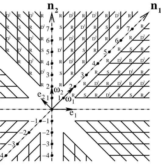
The Kac table of the theory Z5 is shown in Fig. 7, together with the vectors

~e1, ~e2 representing the screening operators of the associated (assumed) Coulomb gas

representation. The labeling of each vertex of the lattice encodes the nature of the corresponding operator: singlet (S), doublet 1 (D1_{), doublet 2 (D}2_{) and disorder operator}

n

₂

n

₁

e

₂

e

₁

1

ω

2

ω

7

6

5

4

3

2

1

−2

−3

−4

−1

2

3

4

5

6

7

−1

−2

−3

−4

1

Fig. 7.— Kac table of the Z5theory, based on the weight lattice of B2. The lattice is spanned

by (one half of) the fundamental weights ~ω1, ~ω2. We show here the “basic layer”, i.e., the

one with (n0

1, n02) = (1, 1). Each vertex of the lattice is labeled according to the nature of

the associated operator (S, D1_{, D}2_{, R). This labeling extends periodically throughout the}

lattice. The simple roots, ~e1 and ~e2, act as screening operators and are associated with

lattice reflections (see text). The arrows give examples of pairs of operators which are linked by such reflections. The physical part of the spectrum is restricted to the wedge limited by the n1 and n2 axes.

It should be observed that the Kac table of the theory Z5 is in fact four-dimensional,

made of two-dimensional layers corresponding to the α+ and α− parts of Eq. (3.1). This

separation on the α+ and α− parts is seen more explicitly from the following form of the

Kac formula: ∆(n1,n2)(n01,n02) = · ³n₁ 2 ~ω1+ n2 2 ~ω2 ´ α++ µ n0 1 2 ~ω1+ n0 2 2 ~ω2 ¶ α− ¸2 − ~α20+ B. (4.1)

In Fig. 7 only one layer is displayed, namely the one with either (n0

1, n02) = (1, 1) or

(n1, n2) = (1, 1). We shall refer to the layers (n1, n2)(1, 1) or (1, 1)(n01, n02) as the “basic

layer” of the Kac table, corresponding to either the α+ or the α− part of the spectrum.

Such a layer is basic in the sense that the other side has trivial indices.

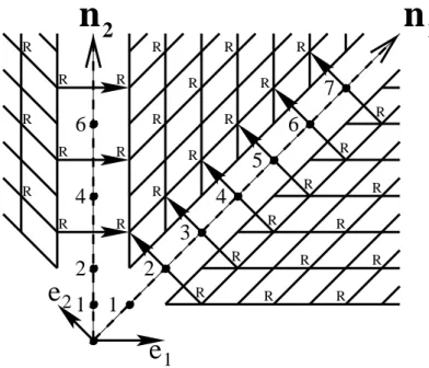
Also shown on Fig. 7 are examples of reflections, marked by arrows pointing from the domains on the left and on the right into the physical domain, which is the upper-right corner of the table (the wedge limited by the n1 and n2 axes). Just like in Felder’s

resolution for minimal (Virasoro algebra) models [8], these reflections, realised by integrated screenings, indicate singular states (degeneracies) in the modules of physical operators. In this sense the operators in the adjacent domains are all “ghosts”, which decouple from the physical operators in the operator algebra, and in correlation functions. As usual, for the above reasoning based on reflections to be justified, we must assume that the screenings commute with the parafermionic algebra.

We can check these assumptions by looking at the low-lying operators in the basic layer of the Kac table, cf. Fig. 7. For the first operators of each type—R (disorder), D2

(doublet 2), D1 _{(doublet 1) and S (singlet)—the levels of degeneracy have been defined in}

Section 2 by direct calculation. Alternatively, the levels of degeneracy could be found, if our assumptions are correct, by taking the difference of the dimensions ∆(n1,n2)(n0₁,n0₂), as given

by Eq. (3.5), for two operators at the ends of the arrow representing a particular reflection in Fig. 7.

For the operator R, positioned as Φ(1,2)(1,1) or Φ(1,1)(1,2), both reflections gives the result

1/2 for the difference of the dimensions:

∆(1,1)(−1,4)− ∆(1,1)(1,2) = 1 2, (4.2) ∆(1,1)(3,−2)− ∆(1,1)(1,2) = 1 2. (4.3)

This agrees with the finding of Section 2 that these disorder operators are doubly degenerate at level 1/2.

Next, for the operator D1_{, at the location Φ}

(1,1)(1,3), one finds ∆(1,1)(−1,5)− ∆(1,1)(1,3) = 2 5, (4.4) ∆(1,1)(4,−3)− ∆(1,1)(1,3) = 4 5, (4.5)

according to Fig. 7. This is in agreement with the fact that this operator is degenerate at levels 2/5 and 4/5, as we have found in Section 2.

In a similar way, the two reflections for the operator D2_{, located as Φ}

(1,1)(2,1), confirm

the degeneracy at levels 1/5 and 1, as found in Section 2. And finally, in the case of the identity operator Φ(1,1)(1,1) = I, which is of the S type, the two reflections in Fig. 7 give the

differences of dimensions 2/5 and 3/5, in accordance with the levels of degeneracy in the identity operator module as dressed in Section 2.

It is important to note that the labeling of the ghost operator, as being R, S, D1 _{or D}2

for every reflection, has to be in accordance with the nature of the corresponding state in the module of the physical operator into which the ghost operator is mapped. For instance, in the module of a D1 _{operator, cf. Fig. 5, a degenerate state at level 2/5 is a singlet,}

because that level belongs to the charge sector q = 0. Likewise, a doublet of degenerate states at level 4/5 (charge sector q = ±2) corresponds to a doublet 2 operator. Evidently, the differences of dimensions, as found in Eqs. (4.2)–(4.5), are to be calculated with the

appropriate boundary terms [identified in Eq. (3.10)] in the Kac formula for ∆(n1,n2)(n0₁n0₂),

cf. Eq. (3.5).

The disorder operators have to map among themselves, assuming that the screening operators which realise the mappings (reflections) do not translate order to disorder.

So far we have identified the nature of the following operators, situated at the low-lying corner of the physical domain shown in the table of Fig. 7:

Φ(1,1)(1,1) = S = I, (4.6)

Φ(1,1)(2,1) = D2, (4.7)

Φ(1,1)(1,2) = R, (4.8)

Φ(1,1)(1,3) = D1. (4.9)

Similar identifications apply on the side of α+, e.g., Φ(2,1)(1,1) = D2 etc. We now show how

to fill in the rest of the basic layer, on the α− side for instance, by making use of simple

fusion rules and reflections.

We first consider the operator product

R · D1 = Φ(1,1)(1,2)· Φ(1,1)(1,3). (4.10)

On the left-hand side, the result of the multiplication should be a disorder operator. On the right-hand side, according to the Coulomb gas rules, the above multiplication produces an operator, in the principal channel, with

~

β(1,1)(1,4)= ~β(1,1)(1,2)+ ~β(1,1)(1,3). (4.11)

Multiplication of operators corresponds to addition of the corresponding vectors ~β in Fig. 7. The non-principal channels follow the principal one by shifts realised by the vectors −~e1

and −~e2. But for the present purposes it will be sufficient to follow the principal channel

At this point we should remark on a sign convention concerning the orientation of

the vectors in the Coulomb gas representation. According to Eq. (3.2), the vectors ~β

have a negative projection along the fundamental weight vectors ~ω1 and ~ω2. The usual

convention in the Colomb gas representation analysis is to change their sign, i.e., to orient them positively, as seen on Fig. 7. To compensate for this convention, the moves associated with the screenings should then be realised by shifts in the direction opposite to that of the simple roots, i.e., in the direction of the vectors −~e1 and −~e2. Without this convention for

the inversion of directions, in the graphical representation of Fig. 7, the Kac table should have been spanned by the vectors −~ω1/2 and −~ω2/2, according to Eq. (3.2). With this

convention in mind, the graphical addition [with respect to the origin (1, 1)(1, 1)] of the lattice vectors in Fig. 7, corresponding to the operators Φ(1,1)(1,2) and Φ(1,1)(1,3) in Eq. (4.10),

is in accordance with the additions of the vectors ~β in Eq. (4.11).

As a result, Eq. (4.10) leads us to conclude that the site (1, 1)(1, 4) of the Kac table is occupied by an operator of type R (disorder).

Next, we consider multiplying the operator D1 _{= Φ}

(1,1)(1,3) with itself:

D1_{· D}1 = Φ(1,1)(1,3)· Φ(1,1)(1,3). (4.12)

The right-hand side produces, in the principal channel, the operator Φ(1,1)(1,5). According to

the left-hand side, this operator has to be either of the D2 _{or the S type. The result D}2 _is

obtained if both D1 _{operators of the left-hand side of Eq. (4.12) belong to the q = +1 part}

of the doublet (or if both have q = −1). However, if the Z5 charge of the two D1 operators

are opposite (one being q = +1 and the other q = −1), the left-hand side produces a singlet (S) operator.

This ambiguity is due to the fact that the site in the Kac table labeled D1 _{is in fact}

the position of both members of the doublet 1, viz. operators with q = ±1. A similar

in the Kac table labeled R accommodates the whole quintuplet {Ra, a = 1, ..., 5} of disorder

operators, all sharing a particular value of the conformal dimension ∆.

The ambiguity for assigning the correct label to the operator Φ(1,1)(1,5) is resolved

by adding an argument based on reflections. In fact, one can check that the horizontal reflection in Fig. 7—from the ghost site on the left, across the n2 axis, and to the site

(1, 1)(1, 5) on the right—has a “bare gap” of

∆(0)_{(1,1)(−1,7)− ∆}(0)_(1,1)(1,5) = 1

2. (4.13)

(Here, we have defined the “bare” dimensions as ∆(n1,n2)(n01,n02)− B, i.e., by Eq. (3.5) with

the boundary term being neglected.)

Suppose first that Φ(1,1)(1,5) is a D2, so that we shall have to correct the second term in

Eq. (4.13) by the boundary term BD2 = 3/20. One now examines in turn the three possible

assignments (D1_{, D}2 _{or S) of a label for the ghost site at (1, 1)(−1, 7), each time correcting}

the first term in Eq. (4.13) by the corresponding boundary term. In case of a consistent assignment, the right-hand side must equal a level on which a ghost operator of the given

nature can be a submodule of the physical D2 _{operator. According to Fig. 6, these levels}

can be: 1/5+integer if the ghost is a D1_{, 3/5+integer if it is a S, and 1+integer if it is a}

D2_{. It is easily verified that none of the three possible assignments leads to a consistent}

result. Therefore, Φ(1,1)(1,5) cannot be a D2 operator.

On the other hand, if Φ(1,1)(1,5) is a singlet, and the calculation of the gap in Eq. (4.13)

is corrected by assuming a (ghost) operator of type D1 _{at the site (1, 1)(−1, 7), then the}

corrected gap in Eq. (4.13) will give 3/5. It is seen from Fig. 4 that a singlet operator can

indeed accommodate a D1 _{submodule at level 3/5. Moreover, D}1 _{is the only consistent}

labeling of the ghost operator.

(and also that the ghost operator Φ(1,1)(−1,7) is a doublet 1).

At the other border of the physical domain, which is parallel to the n1 axis, by using

a similar series of arguments one concludes that the operator Φ(1,1)(3,1), situated next to

D2 _{= Φ}

(1,1)(2,1), can only be a singlet. More precisely, in this case the bare gap for the

reflection across the n1 axis reads:

∆(0)_{(1,1)(4,−1)− ∆}(0)_(1,1)(3,1)= 1

4 (4.14)

By correcting this formula by boundary terms, it can be checked that the only labels that can be consistently assigned to the sites (1, 1)(4, −1) and (1, 1)(3, 1) are those given in Fig. 7.

Having defined the positions of the first nontrivial singlets, i.e., the operators Φ(1,1)(3,1)

and Φ(1,1)(1,5), we can now extend the singlets over the whole lattice (the basic layer in

Fig. 7). To this end, it suffices to multiply the singlets among themselves. In the products they produce only singlets, and we shall cover the lattice by adding the corresponding lattice vectors. Put differently, the lattice vectors corresponding to the operators Φ(1,1)(3,1)

and Φ(1,1)(1,5) are the fundamental ones for the sublattice of singlet operators.

Next, we can extend the labeling D2 _{of the site (1, 1)(2, 1) out over the entire lattice.}

This is done by multiplying Φ(1,1)(2,1) by all possible singlets. As the singlet consists of only

one q = 0 state, the argument based on addition of Z5 charges involves no ambiguity, and

the result can only be another D2 _{operator. As a consequence, every fourth row parallel to}

the n1 axis (viz., the rows 1, 5, 9, . . .) become completely filled out by an alternation of S

and D2 _{operators; see Fig. 7.}

It is equally easy to extend the positions of disorder operators over the whole lattice.

First, multiplying the operator D1 _{= Φ}

(1,1)(1,3) by the basic disorder operator

operators Φ(1,1),(2,2) and Φ(1,1),(2,4) are also disorder operators. This is seen by multiplying

the first two disorder operators, Φ(1,1)(1,2) and Φ(1,1)(1,4), by the basic doublet, D2 = Φ(1,1)(2,1).

Second, the above four disorder operators can be extended throughout the lattice by multiplying them by all possible singlets. In all cases, the result must be a disorder operator. We conclude that every second row of the physical domain is occupied exclusively by disorder operators, as shown on Fig. 7.

At this point, only the rows 3, 7, 11, . . . in the basic layer remain to be determined. In fact, once the nature of the operators Φ(1,1)(1,3) and Φ(1,1),(2,3) is determined, these two

operators can be extended throughout the entire lattice by repeated multiplication by the two fundamental singlets, at positions (1, 1)(3, 1) and (1, 1)(1, 5). The result will be that the rows in question will realise an alternating sequence of these two operators.

The operator Φ(1,1)(1,3) is, of course, already known: it is the fundamental doublet 1

(D1_{). It remains to define Φ}

(1,1),(2,3). Actually, by assuming the whole lattice—and not

just the physical domain—to be filled out in a homogeneous (periodic) way, we could equivalently ask for the labeling of Φ(1,1)(2,−1), four rows below. Now, by consistency of

reflections with the levels in the module of the identity operator S = I = Φ(1,1)(1,1), the

ghost operator Φ(1,1)(2,−1) has to be D2. It is easy to check that this accounts for the

degeneracy at level 2/5. The identification of Φ(1,1)(2,3) as a doublet 2 operator is also

confirmed by a direct degeneracy calculations given in Appendix D.

We thus reach the conclusion that the rows 3, 7, 11, . . . in the basic layer are occupied by an alternation of D1 _{and D}2 _{operators, as shown on Fig. 7.}

Conclusion: By a series of arguments described above, where we have combined reflections and simple fusion rules, we have filled the whole lattice corresponding to the basic layer. The result is shown in Fig. 7.

The sites in the other layers, in which the indices of ∆(n1,n2)(n0₁n0₂) are nontrivial on both

the α+ and the α− sides, must also be assigned S, D1, D2 and R labels. We now show how

this can be accomplished by shifting the labels assigned to the basic layer.

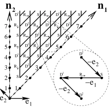
Let us assume, for definiteness, that the lattice in Fig. 7 corresponds to the operators on the α− side, i.e., the operators Φ(1,1)(n0

1,n02) whose indices on the α+ side are trivial,

n1 = n2 = 1. Now consider, for instance, the operators Φ(1,2)(n0

1,n02) having the “excitation”

(1, 2) on the α+ side. In this case the assignment of S, D1, D2 and R labels to the

corresponding two-dimensional lattice with coordinates (n0

1, n02) is simply obtained by a

shift of the distribution of S, D1_{, D}2 _{and R in the basic layer (see Fig. 7) along the vector}

(1, 2). The result is shown in Fig. 8.

Put otherwise, the label of a generic operator Φ(n1,n2)(n0₁,n0₂) only depends on the

differences of indices, (n1− n01, n2− n02). Therefore, the label of Φ(n1,n2)(n01,n02) coincides with

that of Φ(1,1),(n0

1+1−n1,n02+1−n2). As this latter operator belongs to the basic layer, depicted in

Fig. 7, the corresponding label is known.

We remark that the above shifting argument could just as well have been used to trivialise the indices on the α− side. Thus, the label of Φ(n1,n2)(n01,n02) not only coincides

with that of Φ(1,1),(n0

1+1−n1,n02+1−n2) but also with that of Φ(n1+1−n01,n2+1−n02)(1,1). Both these

latter operators belong to the basic layer, since the distinction between the α+ and α−

sides is just a convention. We can therefore conclude that the labels of Φ(1,1),(1+˜n1,1+˜n2) and

Φ(1,1),(1−˜n1,1−˜n2) coincide, for any integers ˜n1 and ˜n2.

The presentation described above—and in particular the notions of “basic layer” and “other layers”—is of course just one particular way which we have chosen to visualise the four-dimensional lattice of operators Φ(n1,n2)(n01,n02).

n

₂

n

₁

e

₂

e

₁

1

ω

2

ω

7

6

5

4

3

2

1

−2

−3

−4

−1

2

3

4

5

6

7

−1

−2

−3

−4

1

Fig. 8.— Assingment of labels to the operators in the layer Φ(1,2)(n0

1,n02). This is obtained by

4.2. Finite Kac tables for unitary theories

All the discussion so far on the Kac table applies in general, when the parameters α+

and α− = −1/α+ take general values. As usual, when α2+ takes rational values, the Kac

table becomes finite. For unitary theories3 α2+= (p + 2)/p, cf. Eqs. (2.62) and (3.3), with p

being an integer. The physical operators’ part of the Kac table will then be delimited by: 2 ≤ n0

1+ n02 ≤ p + 1,

2 ≤ n1+ n2 ≤ p − 1. (4.15)

This is similar to the Kac table of the conformal theory W B2, defined, among other W

theories, by Fateev and Lukyanov in Ref. [9]. The contents of this conformal theory (W B2) and the one considered in the present paper (Z5, second solution) are completely

different. Still, both of them use the weight lattice of the algebra B2 for their respective

representations. And the global properties of their representation lattices (the Kac tables) are the same.

The delimitations of the Kac table of the theory Z5, as given in Eq. (4.15), can also be

checked directly. To this end, we consider reflections in the direction

2~e2+ ~e1. (4.16)

Using Eq. (3.5) for ∆(n1,n2)(n01,n02), together with the appropriate boundary terms established

above, one finds that the operators above the line n0

1+ n02 = p + 2 (4.17)

in Fig. 7 are all ghosts, which should decouple. Their dimensions differ from those of their partners with respect to the reflections in the line (4.17) by values which are consistent

3_{Unitarity is ensured by the existence of the corresponding coset construction; see}

with the levels in the corresponding modules. These reflections are realised by screenings that are units of the vector (4.16) [which is itself made out of three screenings]. This is sufficient to decouple the operators above the line (4.17).

In giving this argument, we have referred to Fig. 7, which is the basic layer of the Kac table. But the argument is true for the other layers as well.

Finally, the remaining finite part of the Kac table, delimited by the conditions in Eq. (4.15), possesses a further symmetry. Using Eq. (3.5) together with appropriate boundary terms, one can check that the operation

   n0 1 → p + 2 − n01− n02, n02 → n02, n1 → p − n1− n2, n2 → n2, (4.18) is a symmetry of ∆(n1,n2)(n0₁,n0₂).

It is also a symmetry of the Kac table of W B2 [9]. The basic difference of the theory

Z5, from a very general point of view, resides in its boundary terms for the different sectors.

The important point is that the symmetry (4.18), as well as the decoupling of the operators outside of the domain (4.15), remains unbroken by the S, D1_{, D}2_{, R structure of the lattice.}

Rather, it is consistent with it.

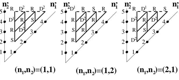
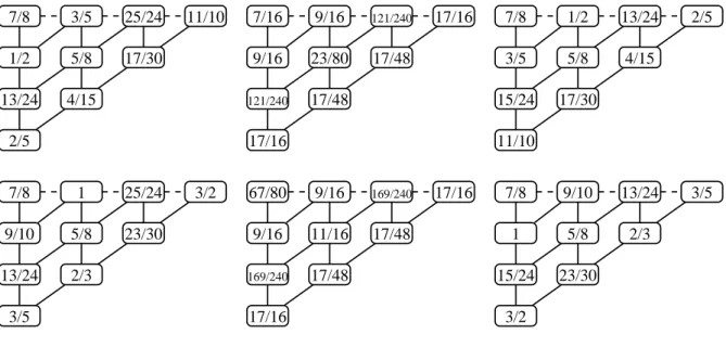
Let us give a simple example of the series of theories that we have constructed. According to the coset formula in Eqs. (1.1)–(1.3), the first non-trivial Z5 theory should be

that with p = pmin = 4, having c = 3/2. Its Kac table, which is made of three α− layers, is

shown in Fig. 9.

The preceding theory, the one with p = 3, is trivial. Its Kac table is made of just one α− layer, with all the operators being present (S, R, D1, D2) having the trivial scaling

dimension, ∆ = 0. This could have been anticipated, because the central charge of this theory is c = 0, according to Eq. (1.2).