Design of an ARQ/AFEC link in the presence of propagation delay and fading

Design of an ARQ/AFEC Link in the Presence of Propagation Delay and Fading

by

Bradley Bisham Comar

B.S., Electrical Engineering (1995) Massachusetts Institute of Technology

Submitted to the Department of Electrical Engineering in Partial Fulfillment of the Requirements for the Degree of

Master of Engineering in Electrical Engineering at the

Massachusetts Institute of Technology June 2000

Q2000 Bradley Bisham Comar. All rights reserved.

The author hereby grants to MIT permission to reproduce and distribute publicly paper and electronic

copies of this thesis document in whole or in part.

Signature of Author:

Depa' ftment of Electrical Engineering May 17, 2000

Certified by:

Dr. Steven Finn Principal earch Scientist

T esisjupervisor

Accepted by:

Arhur C. Smith

Professor of Electrical Engineering Chairman, Committee on Graduate Students

MASSACHUSETTS INSTITUTE OF TECHNOLOGY

JUL

2 7 2000

MIT Libraries

Document Services

DISCLAIMER OF QUALITY

Due to the condition of the original material, there are unavoidable

flaws in this reproduction. We have made every effort possible to

provide you with the best copy available. If you are dissatisfied with

this product and find it unusable, please contact Document Services as

soon as possible.

Thank you.

The images contained in this document are of

the best quality available.

Design of an ARQ/AFEC Link in the Presence of Propagation Delay and Fading

by

Bradley Bisham Comar

Submitted to the Department of Electrical Engineering on May 18, 2000 in Partial Fulfillment of the Requirements for the Degree of Master of Engineering in

Electrical Engineering

ABSTRACT

This thesis involves communicating data over low earth orbit (LEO) satellites using the Ka frequency band. The goal is to maximize throughput of the satellite link in the presence of fading and

propagation delay. Fading due to scintillation is modeled with a log-normal distribution that becomes uncorrelated with itself at 1 second. A hybrid ARQ/AFEC (Adaptive Forward Error Correction) system using Reed-Muller (RM) codes and the selective repeat ARQ scheme is

investigated for dealing with errors on the link. When considering links with long propagation delay, for example satellite links, the delay affects the throughput performance of an ARQ/AFEC system due to the lag in the system's knowledge of the state of the channel.

This thesis analyzes various AFEC RM codes (some using erasure decoding and/or iterative decoding) and two different protocols to coordinate the coderate changes between the transmitter and receiver. We assume the receiver estimates the channel bit error rate (BER) from the data received over the channel. With this BER estimation, the receiver decides what the optimal coderate for the link should be in order to maximize throughput. This decision needs to be sent to the transmitter so that the transmitter can send information at this optimal coderate. The first protocol investigated for getting this information back to the transmitter involves attaching a header on every reverse channel packet to relay this information. The second protocol we explore leaves the information packets unchanged and makes use of special control packets to coordinate the rate changes between the transmitter and receiver.

Thesis Supervisor: Dr. Steven Finn Title: Principal Research Scientist

TABLE OF CONTENTS

1.0 INTRODUCTION

2.0 PHASE I: FINDING AN ADAPTIVE CODE

2.1 Procedure and Results of Phase I

3.0 ANALYSIS OF THE 1-D HARD ADAPTIVE CODE

4.0 PHASE II: ARQ/AFEC IN A FADING ENVIRONMENT 5.0 CONCLUSION

1: BACKGROUND

la) Binary Fields

1b) Vector Spaces lc) ld) le) lf) lg) -dh)

Linear Block Codes Reed-Muller Codes

Bit Error Rate Performance Erasures and Soft Decision Iterative Decoding

ARQ and Hybrid Systems

APPENDIX 2: C PROGRAMS TO SIMULATE PHASE I CODES

2a) C Program for 1-D Hard Code Simulation 2b) C Program for 2-D Soft Code Simulation

APPENDIX 3: PHASE II THROUGHPUT CALCULATION PROGRAM

APPENDIX 4: MARKOV CHAIN MODEL & ITS AUTO-CORRELATION 73 APPENDIX 5: PHASE II THROUGHPUT SIMULATION PROGRAM 75

REFERENCES: 79 7 11 14 19 23 43 APPENDIX 45 47 49 51 53 57 59 61 62 63 63 67 71

1.0 INTRODUCTION

This thesis involves communicating data over low earth orbit (LEO) satellites using the Ka frequency band. The goal is to maximize the throughput of the satellite link in the presence of long propagation delay. It is assumed that the communication system uses power control to negate the effects of fading due to rain attenuation. However, fading due to scintillation must be dealt with. This fading is modeled with a log-normal distribution that becomes

uncorrelated with itself at 1 second.

When communicating digital information over noisy channels, the problem of how to handle errors due to noise must be addressed. The two major schemes for dealing with

errors are forward error correction (FEC) and automatic retransmission request (ARQ) [8]. Combining these schemes into a hybrid ARQ/FEC system can be used to make more

efficient communications over the link [8]. Additional performance is gained by using an adaptive FEC, or AFEC,

scheme which changes coding rate as the signal to noise ratio in the channel changes in order to maximize

throughput performance. Throughput performance is also gained by using the selective repeat ARQ scheme, which our

system uses. Throughput is defined as the inverse of the average number of transmitted bits required to successfully

send one bit of information. When considering links with long propagation delay, for example satellite links, the delay affects the performance of an ARQ/AFEC system due to the lag in the system's knowledge of the state of the

channel.

This thesis addresses some of the analysis that a designer of such an ARQ/AFEC system should consider. The two main phases of this thesis are 1) to analyze various

AFEC codes and 2) to analyze different protocols to

coordinate the coderate changes between the transmitter and receiver. A good AFEC code is determined from phase 1 of this project and then a good coordination protocol for this chosen AFEC is determined in phase 2. Our hybrid ARQ/AFEC scheme uses a CRC check code for error detection in

addition to the AFEC code for error correction.

In phase one, a set of codes is chosen to construct the AFEC code. Here, the major focus is on linear Reed-Muller (RM) codes and two-dimensional (2-D) product codes constructed with these RM codes. 2-D product codes are

explored because literature indicates that they are

efficient and powerful [9].

Because the sizes of 2-D codes

are the square of the sizes of the codes that construct

them, these constructing codes should be limited to

reasonably small sizes.

RM codes are chosen to construct

these 2-D codes because they are optimal at smaller sizes

[5] and they have the added benefit of a known hard

decision decoding algorithm that is faster and simpler than

other comparable block codes [12].

In addition to hard

decision decoders, another set of decoders implements soft

decision (erasure) decoding. This decoding method allows

for three decision regions.

Erasure decoding is proposed

because this decoding method allows for easy and efficient

hardware or software implementation [12].

Therefore, the

four sets of codes explored are normal RM codes with hard

decision decoders, 2-D RM codes with hard decision

decoders, normal RM codes with erasure decoders, and 2-D RM

codes with erasure decoders.

The second phase of this thesis involves incorporating

the AFEC code chosen in phase one with the selective repeat

ARQ scheme.

Sufficient buffering to avoid overflow is

assumed on both the transmit and receive sides of the

channel. The fading on our channel is assumed to be

log-normally distributed. Two different protocols to handle

the change in the AFEC coderate are analyzed. We assume

the receiver estimates the channel bit error rate (BER)

from the data received over the channel.

With this BER

estimation, the receiver decides what the optimal coderate

for the link should be in order to maximize throughput.

This decision needs to be sent to the transmitter so that

the transmitter can send the information at the optimal

coderate.

The first protocol for getting this information back

to the transmitter involves attaching a header on every

reverse channel packet to relay this information. The

header is encoded with the rest of the packet during

transmission. The receiving modem tries decoding every

packet it receives with decoders set at each possible

coderate.

If none or more than one receiver decodes a

packet that passes the CRC check, a failure is declared and

a request for retransmission is issued.

If exactly one

decoder has a packet that passes the CRC check, that packet

is determined good and is passed to the higher layer. A

disadvantage of using this scheme is that every packet has

this additional overhead. This might be a heavy price to

-Vw-pay if the BER is fairly constant for most of the time and the coderate changes infrequently.

The second protocol we explore leaves the information packets unchanged and makes use of special control packets to coordinate the rate changes between the transmitter and receiver. When the receiver wants the coderate of the

transm.1tter to change, it sends a "change coderate" control packet to the transmitter telling it what rate to change to. These packets can be encoded using the lowest coderate which gives the lowest probability of error. Again, the receiver can track the transmitter by using several

decoders and choosing the correctly decoded packet as determined by the CRC code. The benefit of this second protocol over the first protocol described above is more efficient use of the link if the coderate does not change often.

The ARQ/AFEC system under these protocols and log-normal fading is analyzed for throughput. For a fading

model with a mean of 5dB Eb/No and a standard deviation of

2, the better protocol depends on the data rate. For data rates higher than 10 Mbps, the second protocol, which uses control packets, is more throughput efficient. For data rates lower than 2 Mbps the first protocol, which places coderate information in the header, is more throughput efficient. For data rates in between, the choice of protocols does not effect throughput significantly.

2.0 PHASE I : FINDING AN ADAPTIVE CODE

An adaptive FEC code is a code that can change its coderate in response to the noise environment. In this work, an adaptive ARQ/FEC Hybrid system is designed in

order to maximize throughput. During periods of low noise, the system can transmit information at a high coderate and not waste efficiency transmitting too many redundancy bits. During high noise time periods, the system can transmit at a lower coderate and not waste efficiency by

re-transmitting packets too many times. The receiver will monitor incoming packets, estimate the noise environment,

choose which FEC code should be used to maximize

throughput, and relay this information to the transmitter. The first step in designing such a system is to choose an adaptive code. This adaptive code will be a collection of several individual codes with different coderates.

There are many varieties of codes to choose from. This project concentrates on two-dimensional iterative block codes constructed with Reed-Muller codes. See Appendix 1. After looking at different RM codes, the set of codes of

length n=64 is chosen. The RM(1,6), RM(2,6), RM(3,6) and RM(4,6) codes are used. The values of k for these codes are 7, 22, 42, and 57 respectively. Their coderates are 7/64, 22/64, 42/64 and 57/64 and the coderates of the respective 2-D codes they construct are 72/642, 222/642, 422/642 and 572/642. The methods of iterative decoding in this thesis are greatly simplified from traditional

iterative block decoding which is described in Appendix 1g. The RM codes mentioned above are used to create four

2-D codes that use hard decision decoding. These codes are encoded in the normal manner for 2-D codes. See Appendix

1g. The decoding algorithm is as follows. Hard decode all

the columns in the received n x n matrix Ro to create a new

k x n matrix Rv'. Re-encode Rv' to create a new n x n matrix Rv. Rv now has valid codewords for each of its

columns that Ro may not necessarily have. Subtract Rv from

Ro to get Ev. Ev is the error pattern matrix. It will have ls in the locations where the bits in Rv and Ro differ and Os in the locations where they agree. Run this same

procedure with the rows of Ro to create the matrix EH.

Element-wise multiply the two error pattern matrices to create the matrix E. E represents the locations in Ro where

both horizontal and vertical decoding agree are corrupted. Change these bits by subtracted E from Ro. Thus R, = RO-E.

See Figure 1. This procedure can be iterated as many times as desired. After iterating x times, decode R, horizontally to get the k x n matrix R.' and decode the columns of R,' to

get the k x k matrix of message bits. These codes will be referred to as 2-D Hard codes in this paper.

Another set of codes to be analyzed is similar to the set of 2-D Hard codes described above except that decoding

the rows and columns of RO is done with erasure decoding as

described in Appendix 1f. The decoding procedure is as follows. Erasure decode all the columns in the received n x n matrix Ro, which may have erasure (?) bits, to create a new k x n matrix Rv'. Re-encode Rv' to create a new n x n

matrix Rv, which will not have any erasure (?) bits. Perform a special element-wise "erasure addition" on the

two matrices RO and Rv to get a new horizontal matrix Rvx.

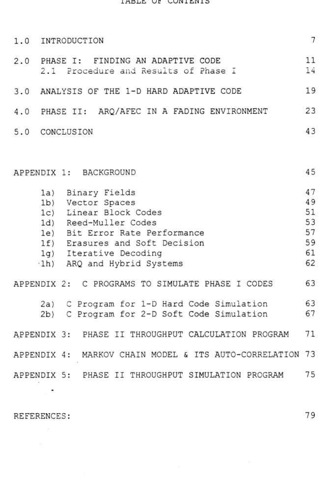
This special addition is labeled as (+) and defined in table 2.1.

1 (+) 0 =? ? (+) 0 = 0 0 (+) 0 = 0

0 (+) 1 = ? 0 (+) ? = 0 1 (+) 1 1

? (+) 1 = 1

1 (+) ? = 1

Table 2.1: The (+) operation.

This addition is intuitively structured so that if one matrix says a bit should 0 and the other says it should be

1, Rvx will determine it undecided or ?. If one matrix is undecided and the other has a solution, that solution is

accepted. Finally, if both matrices have solutions that match, the solution is accepted. Repeat this procedure on

the rows of RO to create RHx. Erasure add RHx and Rvx to create R, = RHx (+) Rvx. This procedure can be iterated as many times as desired. After iterating x times, erasure

decode Rx horizontally to get the k x n matrix R,' and

erasure decode the columns of R.' to get the k x k matrix of

message bits. These codes will be referred to as 2-D Soft codes in this paper. The decision regions that define when a received bit should be decided as a 0, 1 or ? are

determined experimentally.

The last two sets of codes use the same k x k matrix of k2 message bits. These matrices are encoding by encoding each row of the message matrix with the appropriate RM code to create a k x n matrix that gets transmitted to the

Ro (nxn) decode

decode

x

E

This figure shows the procedure for making matrix E in the

decoding algorithm. R1 = RO - E. Note that binary field

subtraction is equivalent to binary field addition. (See Appendix 1b).

receiver.

The received matrix RO can be decoded by hard

decoding each row of RO to regenerate the k x k message

matrix. This set of codes is referred to as 1-D Hard

codes.

See Appendix 2a.

RO can also be decoded by erasure

decoding each row of R

to regenerate the k x k message

matrix. This set of codes is referred to as 1-D Soft

codes. These 1-D codes are used as baseline codes that are

used to evaluate the performance of the 2-D codes described

above.

2.1

Procedure and Results of Phase I

Before analyzing these codes, decision regions for the

soft codes must be determined. The first regions in signal

space that are tried are:

(See Appendix le)

---z---I

-

X---I--- ---

X---choose 0

1 choose ?

I

choose

1

Here, the length of z equals two times the length of y.

Letting a = sqrt(Eb/No) and b = sqrt(energy of signal):

P(error)

=

Q(distance to travel

/

s)

z +

2y

=

3z

=

2b

=>

z =

2b/3

P(erasure or error) = Q(2b/3s) = Q(2a/3)

P(error) = Q(4a/3)

P(erasure) = Q(2a/3) - Q(4a/3)

When these decision regions are tried, the soft decision

decoders perform worse than the hard decision decoders in

both the 1-D and 2-D codes. Therefore, we tried other size

regions to see if performance can be improved. We tried

the following region sizes:

P(error)=Q(0.80a)

P(erasure)=Q(1.20a)-Q(0.80a)

P(error)=Q(0.85a)

P(erasure)=Q(1.15a)-Q(0.85a)

P(error)=Q(0.90a)

P(erasure)=Q(1.10a)-Q(0.90a)

P(error)=Q(0.95a)

P(erasure)=Q(1.05a)-Q(0.95a)

The third row of probabilities works best for the 2-D Soft

codes. This corresponds to a value of z that is (0.22...)y.

For 1-D soft codes, no decision region works well. When

the decision region for ? shrinks to zero, the performance

of this code approaches the performance of 1-D hard codes.

The third row of probabilities is used to calculate the

performance of 1-D soft codes.

Due to a programming mistake found while debugging C

code, a peculiar property with the 2-D soft codes is

discovered. When calculating R, =

(+)

better

performance is gained defining this erasure addition as

shown in table 2.2.

1 (+) 0 = 1 ? (+) 0 = 0 0 (+) 0 0

0 (+) 1 = 0 0 (+) ? = 0 1 (+) 1 1

? (+) 1 = 1

1 (+) ? 1

Table 2.2: A new (+) operation.

When the horizontal and vertical matrices disagree, side

with the horizontal matrix. This new calculation, labeled

while R,

(+)

does.

Thus, the best performance of

these codes is gained when doing Ra

=

(+)

Rvx on the

first n-1 iterations and doing R, =

on

the last

iteration. A value of n=6 seems to work reasonable well.

Going beyond this point requires more calculations and

achieves less benefit form the extra work. In this thesis,

the first five iterations use (+) while the last iteration

used

See Appendix 2b.

Note that this problem is not

horizontal specific. If the rows are decodes first and the

columns second during the iterations, then the best codes

requires siding with the vertical matrix. Therefore, it

does not matter whether the columns or rows are decoded

first as long as (+)x is consistent. In this project, the

columns are decoded first.

Calculating the throughput of these codes under the

selective repeat ARQ scheme assuming sufficient buffering

on both ends to avoid overflow makes use of the throughput

equation: Tsr = PcR where R is the coderate and P, is the

probability that the matrix is decoded correctly. See

Appendix lh.

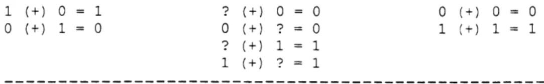
The simulated performance of 1000 matrices

transmitted for each code under each of several different

Eb/Nos is run.

Table 2.3 shows the simulated error

probabilities and Figure 2 shows the throughput performance

graph calculated from these error probabilities.

Codes constructed by RM(1,6):

Eb/NO 1-D Hard 1-D Soft 2-D Hard 2-D Soft

0.2 95.5 95.2 .1 0

0.4 29 26.7 0 0

0.6 1.9 1.8 0 0

0.8 0 0 0 0

Codes constructed by RM(2,6):

Eb/NO 1-D Hard 1-D Soft 2-D Hard 2-D Soft

0.4 100 100 100 100 0.6 100 100 82.5 12.3 0.8 99.6 100 0 0 1.0 90.2 92.8 0 0 1.2 49.2 54.4 0 0 1.4 16.1 19.0 0 0 1.6 3.8 5.4 0 0 1.8 0.9 2.2 0 0 2.0 0.1 0.5 0 0 2.5 0 0 0 0 Codes constructed by RM(3,6):

Eb/NO 1-D Hard 1-D Soft 2-D Hard 2-D Soft

1.2 100 100 100 100 1.4 100 100 99.9 92.4 1.6 100 100 75.4 25.7 1.8 99.1 99.6 15.8 1.3 2.0 91.8 96.3 0.9 0 2.5 31.0 43.8 0 0 3.0 5.6 10.0 0 0 3.5 0.8 1.5 0 0 4.0 0 0.1 0 0 4.5 0 0 0 0 Codes constructed by RM(4,6):

Eb/NO 1-D Hard 1-D Soft 2-D Hard 2-D Soft

2.0 100 100 100 100 2.5 100 100 100 99.6 3.0 98.8 99.9 92.4 69.8 3.5 78.7 91.6 43.2 14.7 4.0 45.0 61.7 10.0 2.0 4.5 17.3 32.2 1.7 0.2 5.0 6.1 14.0 0.2 0 5.5 2.8 6.1 0.1 0 6.0 1.3 2.2 0 0 6.5 0.3 0 0 0

Table 2.3: P(Matrix error) with 1000 packets passed. Eb/No is in the

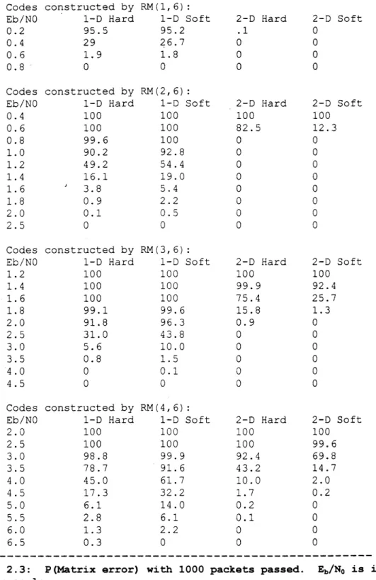
Throughput Performance Curves for the different RM codes

Eb/No

FIGURE 2: These throughput performance curves are obtained by taking the error probability information in table 2.3 and multiplying the

probabilities by the coderates of the respective codes.

From the information in Figure 2, the 1-D hard set of codes is chosen to make the adaptive FEC code. This code does not always perform as well as the 2-D codes, but it comes close. The 2-D codes require much more calculations, and thus they become unattractive. It should be noted that the

2-D codes give much better BER performance, but they

operate with lower coderates which pushes their throughput performance back to levels similar to those of the 1-D hard code.

3.0 ANALYSIS OF THE 1-D HARD ADAPTIVE CODE

The set of 1-D hard codes is modified so that all the codes are the same size. This is a good idea so that the transmitter and receiver do not lose synchronization when coderate information is miss-communicated. Currently, the

k x n matrix sizes vary because the values of k vary.

Therefore, the number of rows needs to be fixed to a value

f. The size of the f x n matrix is -n and it contains 'k

message bits. Another factor to consider is that extra overhead bits are needed. In this project, 64 bits are allocated for a 32 bit CRC-32 checksum, a 24 bit packet number field, and 8 bits for other control information. Therefore, the new coderate of the individual 1-D hard

codes is R=(ke-64)/ne and throughput of these codes is PcR=(1-Pe) (k-64) /ne.

In order to verify the results of the simulated

throughput performance of the chosen code, the union bound estimate is used.

P(row correctly decoded) = P(O bit errors) +

P(l bit error) + P(2 bit errors) + ... + .5P (dmin/2 errors)

The last term is added into the equation because when exactly dmin/2 errors occur, the decoder picks one of the two nearest codes and is correct half the time. The decoding is deterministic, but the probabilities of

occurrence of the two codes to decide upon are equal. Note that the codes used in this project all have even dmins. Also note that these equations assume only one nearest neighbor for each codeword. If there is more than one

nearest neighbor, the probabilities calculated will be less than the actual probabilities. Even if there is only one nearest neighbor, other neighbors a bit further away may make the union bound estimate smaller that the actual probabilities. The calculated probabilities of correctly decoded rows are:

P(for RM(4,6)) = x64 + Comb(64 1) (l-x)x63 + .5Comb(64 2) (1-x)2 x62 P(for RM(3,6)) = x6 4 + Comb(64 1) (l-x)x63 + Comb(64 2) (1-x) 2 + Comb(64 3) (1-x) x61 + .5Comb(64 4) (l-x) 4x60 P(for RM(2,6)) = x64 + Comb(64 1) (-x)x 63 + P(for RM(1,6)) = x64 + Comb(64 1) (1-x)x63 +

The solutions for these calculations appear in table 3.1. Also in this table is the simulated calculations for 1000

matrices of one row for comparison.

and are traditional RM codes.

Eb/NO 0.2 0.4 0.6 0.8 1.0 1.2 1.4 1.6 1.8 2.0 2.5 3.0 RM (1, 6) 36.6%/58.8% 4.8/ 9.8 0.2/ 7.8 0/ 0.4 0/ 0.2 0/ 0 0/ 0 0/ 0 0/ 0 0/ 0 0/ 0 0/ 0 RM (2, 6) 98.7/99.6 85.7/89.5 56.0/59.0 26.2/27.3 9.2/ 9.5 3.2/ 2.7 0.6/ 6.6 0/ 1.4 0/ 0.3 0/ 0 0/ 0 0/ 0

These matrices have =l

RM (3, 6) 100 / 100 99.9/99.7 96.7/96.5 88.9/85.4 72.9/66.2 54.8/44.8 34.1/27.0 21.0/14.8 10.8/ 7.6 5.4/ 3.7 1.0/ 0.5 0.2/ 0.1 RM (4, 6) 100 / 100 100 / 100 99.9/99.7 98.2/97.9 94.6/92.7 88.3/82.9 80.2/69.8 68.7/55.4 56.0/41.9 41.1/30.4 19.8/12.1 7.8/ 4.4

Table 3.1: 1000 Packet Simulation vs. Analytic Solution. The following table shows the simulated probability of error P(e) data run on the 1-D Hard C program in Appendix 2a with a slight modification. The number of rows is changed from k to 1. A C program is used to calculate the union bound estimate as shown in section 3. The format for the table is (simulated P(e))/

(analytic P (e) ) .

Note that the analytic solutions are close to the simulated solutions. Given that the analysis is an approximation, the simulation algorithm will be used to obtain values for the probability of matrix error. To get more accurate calculations, 100000 matrices (data packets) are

transmitted in the simulation program for each RM code as a

function of Eb/No. The results of these simulations on packets of £=l appear in table 3.2.

For the packets constructed with the RM(2,6) code:

P(e)=0.000 for all Eb/No values tested.

For the packets Eb/No P(e) 0.25dB 6.852% 0.50 4.779 0.75 3.207 1.00 2.013 1.25 1.256 1.50 0.706 .For the Eb/No 0.25dB 0.50 0.75 1.00 1.25 1.50 1.75 2.00 For the Eb/No 0.25dB 0.50 0.75 1.00 1.25 1.50 1.75 2.00 2.25 2.50 2.75 3.00 packets P(e) 67.611% 61.298 54.542 47.494 40.414 33.500 27.204 21.333 packets P(e) 95.026% 93.160 90.860 87.981 84.420 80.180 75.262 69.611 63.344 56.850 50.018 43.186

constructed with the RM(2,6) code:

Eb/No P(e) Eb/No

1.75 0.401 3.25 2.00 0.190 3.50 2.25 0.097 >3.5 2.50 0.038 2.75 0.014 3.00 0.006

constructed with the RM(3,6) code:

Eb/No P(e) Eb/No

2.25 16.186 4.25 2.50 11.895 4.50 2.75 8.414 4.75 3.00 5.803 5.00 3.25 3.722 5.25 3.50 2.370 5.50 3.75 1.413 5.75 4.00 0.815 6.00 >6.0

constructed with the RM(4,6) code:

Eb/No P(e) Eb/No

3.25 36.460 6.25 3.50 30.134 6.50 3.75 24.323 6.75 4.00 19.111 7.00 4.25 14.644 7.25 4.50 10.962 7.50 4.75 7.871 7.75 5.00 5.515 8.00 5.25 3.783 8.25 5.50 2.517 8.50 5.75 1.645 >8.5 6.00 1.038

Table 3.2: 100000 Packet Simulation. The following table shows the simulated probability of error P(e) data run on the 1-D Hard C program in Appendix 2a with 1 row. This simulation differs from the one recorded in table 3.1 because it is run on 100000 packets instead of 1000 packets and Eb/NO is in the dB scale here while it is in a linear scale above. The probabilities of errors here are used to characterize the performance of the 1-D Hard codes.

Our adaptive code, which can code messages at any of

the four coderates discussed above, can also choose not to

code the message at all. To determine the probability of

error for uncoded packets, the simulation program is run

with 100000 packets without encoding or decoding.

The

P(e) 0.001 0.001 0.000 P(e) 0.460 0.244 0.10? 0.04C 0.020 0.007 0.003 0.001 0.000 P(e) 0.603 0.361 0.184 0.096 0.042 0.022 0.015 0.006 0.004 0.001 0.000

following calculations are made to compare with the

simulations. Note that this calculation does not depend on approximations as did the calculations for coded data.

P(row error) = 1-P(good row) = 1-(l-P(bit error) )6 4

[no coding] = 1- (1-Q (sqrt (2E/N,)) ")

= 1- (1-. 5erf c (2E/NO) 6)

= 1-(1-.5erfc(exp(.1(Eb/Noin dB)lnlO)) 4 )

The last line is a trick used because MS Excel does not have an antilog function. The analytic solutions and

simulations at 100000 passed packets match to within %0.1. See table 3.3. This case validates the accuracy of the simulations. For the case where there is no coding, the throughput performance curve uses the analytic solutions and not the simulations. Now that the probability of an error in a row is determined for all codes, the probability of an f row packet error is: P(packet error) = 1 - P(good packet) = 1-P(every row is good) = 1 - [1-P(row error)]'.

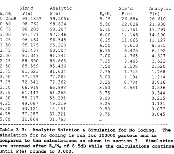
Sim'd Analytic Sim'd Analytic

Ee/NO P(e) P(e) Eb/No P(e) P(e)

0.25dB 99.183% 99.205% 5.25 26.684 26.610 0.50 98.762 98.824 5.50 22.026 21.938 0.75 98.205 98.287 5.75 17.751 17.791 1.00 97.471 97.546 6.00 14.145 14.190 1.25 96.464 96.545 6.25 11.065 11.127 1.50 95.175 95.220 6.50 8.613 8.575 1.75 93.437 93.507 6.75 6.425 6.492 2.00 91.347 91.341 7.00 4.765 4.827 2.25 88.690 88.665 7.25 3.465 3.522 2.50 85.559 85.436 7.50 2.508 2.520 2.75 81.623 81.634 7.75 1.745 1.768 3.00 77.279 77.264 8.00 1.194 1.214 3.25 72.341 72.362 8.25 0.784 0.816 3.50 66.919 66.998 8.50 0.581 0.536 3.75 61.147 61.268 8.75 0.344 4.00 55.217 55.295 9.00 0.215 4.25 49.087 49.219 9.25 0.131 4.50 43.121 43.181 9.50 0.077 4.75 37.287 37.321 9.75 0.045 5.00 31.864 31.763 ...

Table 3.3: Analytic Solution & Simulation for No Coding. The simulation for no coding is run for 100000 packets and is

compared to the calculations as shown in section 3. Simulations are stopped after Eb/No of 8.5dB while the calculations continue until P(e) rounds to 0.000.

4.0 PHASE II: ARQ/AFEC IN A FADING ENVIRONMENT

A log-normal fading environment with an Fb/No that is

constant over the duration of one packet transmission is assumed. The overall throughput over a long period of time

that includes fading is the average of the throughput

performance curve (with Eb/No in dB) scaled by the Gaussian

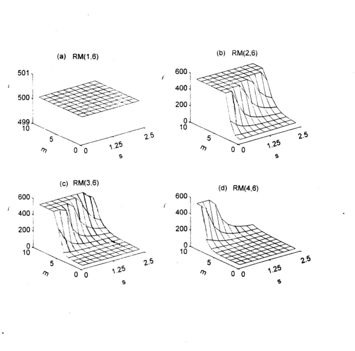
PDF curve of a certain mean m and standard deviation s. MATLAB code is written to calculate this throughput for values of m that range from 1 to 10 in steps of 1 and values of s from .25 to 2.5 in steps of .25. Values of f ranging from 1 to 50C are calculated for each case and the value that gives the optimal throughput for each m and s for each code is recorded in figure 3. The graphs have sections with a ceiling of 500, but the actual optimal

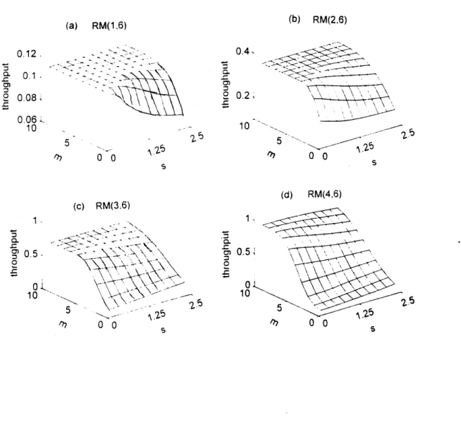
values of f will be higher in these regions. The optimal throughputs at these values of i are shown in figure 4. Figure 5a shows the best throughput for any of the

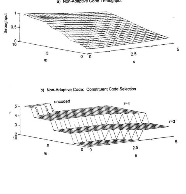
individual codes at each value of m and s. This graph represents the best that can be done in a location with noise characteristics m and s where the system designer can choose any fixed code but not an adaptive code. Figure 5b has a graph that shows which code gives that optimal

performance. Notice that in figure 5, the values of s are extended to 5.0 and the step size of m is decreased to 0.5. Figure 6 shows the performance of an adaptive code and the

value of 4 that should be used for that code. All the

constituent fixed codes that make up the adaptive code have f rows at each value of m and s so that all packets are the same size at each value of m and s. Therefore, picking a

value I for the adaptive code is a compromise that results

in each constituent code not necessarily having the optimal size. Figure 7 shows what is gained by using the adaptive code of figure 6a instead of the best fixed code of figure 5a. The graph shows percent change by plotting throughput of the adaptive code divided by throughput of the fixed code. As expected, when the standard deviation is small, the impact of using the adaptive code is minimal because only one of its constituent codes is running most of the time. As s increases, the adaptive code becomes a better

solution. Appendix 3 shows the program that is used to generate the graphs in figures 3-7.

(a) RM(1,6) 501 5004 499 10 25 "?7 0 0 (c) RM(3,6) 600,! 4001 200 l 10 1_75 0 0 '. (b) RM(2,6) 600 4004 200 0 10 . 0 0 (d) RM(4,6) 600 400 200 10 S2.6 0 0

FIGURE 3: These graphs show the values of t which give the optimal

throughput for 1-D Hard codes in a hybrid selective repeat ARQ scheme.

Values of e are shown for fading environments with mean values of m ranging from OdB to 5dB and standard deviation values s ranging from .25 to 2.S. Note that values of t are restricted to a ceiling of 500.

(a) RM(1,6) (b) RM(2,6) 5 0 0 (c) RM(3,6) 15 505 rh r) S (d) RM(4,6) 0~0.51 10 /77.0 0 0

FIGURE 4: These graphs show the optimal throughput of the constituent

codes at the values of f in figure 3. 0.12 = 0.1. 0 0.08, 0.061 10 -~N \\ 0, 5. 0 0 0.2, 10 S CL 0)

a) Non-Adaptive Code Throughput 0. 0.5 0 10 50 0 ) Ns

b) Non-Adaptive Code: Constituent Code Selection

5 uncoded _r=4 r4 3 21 10 5 51 0S

FIGURE 5: The first graph, figure 5a, is the composite of the optimal throughputs of the constituent codes in figure 4. This graph

represents the best throughput that can be achieved using a

non-adaptive FEC code with selective repeat hybrid system. Figure 5b is a graph that shows which of the constituent codes is used by the adaptive code at each of the different fading environments (at each of the

values of m and s.) Note that the step size of m is decreased co .5dB

and the range of s is extended to 5.

a) Adaptive -ode Throughput

CL

0

0 0 _S

b) Adaptive Code I values 300-, S200 100 0-10 M 0 0 FIGURE 6: 5

The throughputs that are achieved with our adaptive FEC code and selective repeat hybrid system are shown in figure 6a. Figure 6b

is a graph showing the optimal values of 1 at each of the different fading environments. Notice the spikes in this graph where the noise

PDF is sharp (s is low) and is centered on an Eb/No value that is near a

transition point of constituent codes in the AFEC.

0.5

10

Adap. Thru / Non-Adap. Thru. C. = 1.5, 0 1.4 1 *0 S1. 0 C3 1.1> <:7-0 0

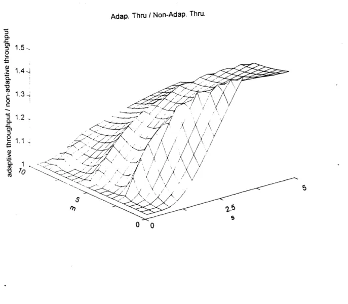
FIGURE 7: This graph shows the ratio of the optimal non-adaptive hybrid system throughput in figure 5a to the adaptive hybrid system throughput in figure 6a. This graph represents how much better an adaptive hybrid code works in different fading environments. Notice that the benefit of using an adaptive hybrid system increases as the standard deviation of the fading environment increases.

To study the effects of propagation delay in the link, we focus on a specific fading model. We choose the fading model with mean m = 5dB and standard deviation s = 2. The

optimal value of f in this case is 18. Figure 8 shows how different values of

e

for the constituent codes that make the AFEC. The

performance of the AFEC is the maximum of these curves. Also shown in this figure is the Gaussian PDF curve of the fading. This curve is not plotted on the same vertical scale as the throughput performance curves. It is included in the figure to give a sense of how often each coderate is used. Notice that the curves are cut off at Eb/NO=OdB. At

zero Eb/NO and below, it is assumed that the modem loses its

lock on the signal and thus the throughput is zero. To explore how a delay in the estimated BER of the noise in the channel affects the overall throughput of the

system, a fading model for Eb/NO with respect to time must

be determined. This delay can be caused by the propagation delay while the estimated coderate information is sent from

the receiver to its transmitter. The model used in this thesis is a Markov Chain model with a Gaussian probability density function. The pertinent Markov Chain equation is:

Pj+j = (Xj/pj+)Pj. The probability of being in state

j,

is determined by the Gaussian function. The probability of staying in the current state is some fixed probability for all states. In this thesis, the probability of staying in

any state is 0.9. This is all the information needed to determine values for X and pi. Appendix 4 has a program that

used these Markov chain calculations. Notice that a chain is created which has a PDF of only the right side of the Gaussian function. At state 0, a coin is flipped to

determine whether the states that the chain visits should be interpreted as left or right of the center of the

Gaussian function. This coin is re-flipped each time state

0 in entered. This trick creates a Markov Chain with a full Gaussian PDF. Each time the chain makes a decision to enter a new state or stay in the current state, an

iteration occurs. The chain is allowed to run for various numbers of iterations to determine how many iterations it takes for the PDF to look like a Gaussian function. See figures 10-12.

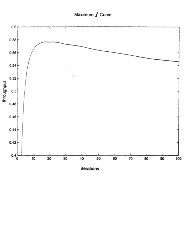
Maximum

I

FIGURE 8: This graph shows the throughput performance of an adaptive .EC selective repeat ARQ hybrid system with the specific fading

characteristics of m = 5dB and s = 2 for different values of f.

Throughput is maximized for f = 18. Therefore, the packet size of our

Constituent Curves 1- 0 000uncoded

0

0

0

0

0

FIGURE 9: This graph shows the performance curves of the constituent codes that make up the AFEC at e=18. The performance of the AFEC is

simply the maximum of these curves at each Eb/Nq value. The curve drawn

in the circled line is the PDF of the fading at mean m = 5dB and standard deviation s = 2. This PDF curve is not drawn to scale vertically.

a) Fade 0 100 200 300 400 500 iterations b) Prob. Density 0 0 2 4 6 8 10 12 14 16 18 20

FIGURE 10: The output of the Markov Chain run for 1000 iterations

modeling a fade with m=5dB and s=2 is shown in figure 10a. Figure 10b

is the calculated PDF for this chain. Because it does not look like

the expected Gaussian curve, more iterations should be run.

6 5.5 5 4.5 4 3.5 3

0

0

0

0

0

0

0

0

0

0

a) Fade 0 1000 2000 3000 4000 5000 6000 7000 8000 9000 10000 iterations b) Prob. Density a-0 0 0 0 0 0 0

0

0

0

FIGURE 11: The output of the Markov Chain run for 10, 000 iterations modeling a fade with m=5dB and s=2 is shown in figure Ila. The PDF curve in figure llb looks more like the Gaussian curve. However, more iterations should be run.

6-

~

5

3- 2-CD

a) Fade 10 8 6 2 0 U-0 0L 0

0

FIGURE 12. The output of the Markov Chain run for 25,000 iterations modeling a fade with m=5dB and s=2 is shown in figure 12a. The PDF curve in figure 12b looks more like the Gaussian curve.

Auto-correlation graph 3.5, 3 2.5 2 1.5 0 1000 2000 3000 4000 5000 6000 7000 8000 9000 10000 iterations

FIGURE 13: This graph shows the auto-correlation RA = E [A (t) 'A (t+T) I of

the output of the Markov Chain run for 100,000 iterations. The

expected value is taken by averaging over 90,000 iterations. T ranges

from 0 to 10,000 iterations. The output becomes uncorrelated with

itself at about 2000 iterations. 1

0.5 0 -0.5

At this point in the thesis, an absolute time scale for the iterations of the Markov Chain model is set using

an auto-correlation function, RA(T) = E[A(t+T)A(t)I. See

Appendix 4. This function determines how well the Eb/No at one point in time is correlated with the Eb/No T iterations

later. The results are shown in figure 13. The noise becomes uncorrelated with itself at approximately 2000

iterations. This cutoff will be defined as 1 second to approximate the affects of scintillation on Ka band

signals. It is assumed that fading due to rain attenuation is handled by power control or some other means. Thus, 2000 iterations of a Markov Chain corresponds to 1 second of time.

The affects of delay and the different protocols to

relay channel Eb/No information from the receiver to the transmitter can now be simulated. MATLAB code is run to

simulate the affects of delay on throughput. See Appendix

5. The choice of running this simulation for 1 million

iterations or 500 seconds is determined by running

simulations with zero delay for varying amounts of time and seeing how close the simulations' throughputs come to the calculated throughputs of the program in Appendix 3. The results are listed in table 4.1.

#iteratons throughput

#iteratons

100K .5868 850K .5927

400K .6099 1000K .5871

600K .5890 1500K .5837

---Table 4.1: This table shows the number of iterations for which

the Markov Chain fading model is run and the associated system throughput calculated. m = 5dB, s = 2, t = 18.

From this table, it looks as though 1000K iterations is where the throughput starts to stabilize near the .5766

calculated throughput target. The calculated PDF for 1 million iterations also looks Gaussian. The program in Appendix 5 is run for several different delays and the

results are listed in table 4.2. This information is graphed in figure 14. These throughputs do not take into account the BER information that gets passed over the link from the receiver to its transmitter. This plot represents the baseline curve because any protocol for transferring BER information will not be able to perform better than the throughputs in this curve. Also shown on this graph is

another simulation that only differs in the number of

bits of information represent the extra space in the header

of each packet that would be used to relay coderate

information from the receiver back to the transmitter in

the return link. Because the link is bi-directional, the

extra overhead will be added on packets in both directions.

To simulate the protocol in which control packets are

used to relay coderate information as opposed to an

increased header, the data rate for the link must be known.

This simulation is done for data rates of 1 Gbps, 10 Mbps,

and 2 Mbps.

Because a packet is roughly 1000 bits

(=18)'(n=64), 1 Gbps represents 1 million packets per

second or 500 packets per iteration. Thus, each iteration

represents the passing of 500 packets while sending a

control packet only costs 1 packet worth of information.

Following the same reasoning, the 10 Mbps data rate leads

to 5 packets per iteration and the 2 Mbps leads to 1 packet

per iteration.

The throughputs for these links are shown

in table 4.2.

header control packet protocol baseline protocol 1 Gbps 10 Mbps 2 Mbps delay thruput thruput thruput thruput thruput

0 .5871 .5809 .5871 .5806 .5817 25 .5788 .5726 .5788 .5777 .5735 50 .5719 .5658 .5719 .5709 .5667 75 .5653 .5593 .5653 .5643 .5602 100 .5592 .5532 .5592 .5581 .5541 200 .5387 .5330 .5387 .5378 .5338 300 .5246 .5190 .5246 .5237 .5198 400 .5127 .5072 .5126 .5117 .5080 500 .5029 .4975 .5029 .5020 .4983 1000 .4772 .4721 .4772 .4763 .4729 1500 .4639 .4590 .4639 .4631 .4597 2000 .4547 .4498 .4546 .4538 .4505 2500 .4513 .4465 .4513 .4504 .4472 3000 .4486 .4438 .4586 .4478 .4445 3500 .4493 .4445 .4493 .4485 .4452 4000 .4487 .4439 .4586 .4487 .4445

Table 4.2: This table shows the throughput of the baseline curve in column 2 with respect to the delay in iterations of the Markov Chain. This column does not use any protocol to get coderate information back to the transmitter. Column 3 uses an extra 8 bits in the header to relay coderate information. The last three

columns use control packets to relay coderate information with system data rates of 1 Gbps, 10 Mbps, and 2 Mbps respectively. For all these columns, m = 5dB, s = 2, and f = 18.

The performance plot of the control packet protocol at

1Gbps is indistinguishable from the plot for the baseline

delay curve (figure 14).

At 10 Mbps, the performance plot

of the this protocol is worse than the baseline curve, but

still better than the plot of the curve which represents

passing coderate information in each packet header (figure

15).

At 2 Mbps, the performance of this control packet

protocol is worse than the performance of the header

protocol (figure 16).

However, all these curves are close

to the baseline curve.

Minimizing delay is more important

than the protocol used to relay coderate information from

the receiver back to the transmitter. This delay is

approximately twice the round trip propagation delay of LEO

satellite communications, and therefore is on the order of

.025 seconds or 50 iterations.

1Gbps baseline ctrt pkts -header 500 1000 1500 2000 2500 3000 3500 4000 iterations

FIGURE 14: This graph shows how delay of the channel noise information

affects throughput for a system at bit rate 1Gbps with a fading environment of m=5dB and s=2. The upper curve is the baseline curve and also shows the throughput of the system using the control packet protocol. The second lower curve shows the throughput of the system using the header protocol. Also shown is the throughput of the

calculated adaptive hybrid system at zero delay and the throughput of the non-adaptive hybrid system at zero delay. From these zero delay

lines, we see that the throughput performance of the adaptive system

degrates to that of the best non-adaptive system if the channel

information is delayed for about 1000 iterations or 1 second.

0.6 0.58 0.56 0.54 0.52 0. 0) 0. 0.5 0.48 0.46 0.44 C

10Mbps 0.6 0.58 0.56- .54-c.0.52 o.5 -baseline 0.48-ctrl pkts 0.46- header 0 500 1000 1500 2000 2500 3000 3500 4000 iterations

FIGURE 15: This graph shows how delay of the channel noise information affects throughput for a system at bit rate 10Mbps with a fading

environment of m=5dB and s=2. The baseline curve (upper curve) and the throughput curve of the system using the header protocol (lower curve) do not change. The throughput curve of the system using the control packet protocol (middle curve) starts to move lower. However, this system still performs better than the system that uses the header protocol.

2Mpbs 0.6 0.58 0.56- 0.54-. 0 .52,-0 0.5-baseline 0.48 header ctri pkts 0.44 0 500 1000 1500 2000 2500 3000 3500 4000 iterations

FIGURE 16: This graph shows the same throughput performance curves when the systems are operating at 2Mbps. The curve of the system that

uses control packets has now dropped below the curve of the system that uses the header protocol.

5.0 CONCLUSION

When designing an ARQ/AFEC system, many choices of codes are available to construct the AFEC. If RM codes are chosen, then erasure decoding and/or simple 2-D iterative block decoding do not buy enough throughput performance to make them worth their added complexity. One reason for this may be due to the fact that in an AFEC, codes are run on the edges of their performance curves. The range of

Eb/No values for which a code is used starts near to where that code's throughput performance falls off to zero. This most likely explains why a delay in updating coderate

information in our AFEC has such a dramatic negative effect on throughput. If fading causes the Eb/No to decrease, then

the throughput of the system is falling to zero for a period of time until the new code is selected.

The ARQ/AFEC system under the two protocols and log-normal fading was analyzed for throughput. First a

comparison of the ARQ/AFEC with an ARQ/Non-Adaptive FEC was made to determine whether a system designer should bother

with an adaptive code. Adaptive codes become more worth while as the standard deviation of the fading environment increases. With communications over a LEO satellite, which has a round trip delay on the order of .013 seconds, and a

fading model with a mean of 5dB Eb/No and a standard

deviation of 2, an ARQ/AFEC system makes sense. With this fading model, the better protocol for sending channel

information from the receiver to its transmitter depends on the data rate. For data rates higher than 10 Mbps, the protocol that uses control packets is more throughput efficient. For data rates lower than 2 Mbps the protocol that places coderate information in the header is more throughput efficient. For data rates in between, the choice of protocols does not seem to affect throughput significantly.

These observations introduce two interesting

extensions to this thesis. First, the erasure decoding and

2-D iterative decoding can be tested for throughput

performance at much higher Eb/No values that have error

probabilities on the order of 10-6 and 109. This is the usual region in which non-adaptive codes are used and

analyzed. Our ARQ/AFEC does not run codes in this region because throughput is not maximized by doing so. Better

throughput is achieved by switching to a code with a higher coderate and letting the ARQ system handle much of the

error control. It would be interesting to see if the erasure decoding and iterative decoding methods greatly outperform the normal RM decoding at these higher Eb/NO regions. If they do, one conclusion that may be drawn is that when constructing an ARQ/AFEC system, a designer

should not bother with complex codes that approach the Shannon limit. Simple codes like normal RM codes may be used with minimal loss in throughput performance.

The second interesting extension to this thesis is to use margin when switching from one code to the next code so that the throughput of the system does not fall to zero as quickly during the delay in switching coderates. A range of margins can be analyzed to find the margin that produces the highest throughput.

APPENDIX 1: BACKGROUND

To understand the error correcting codes used in this thesis, binary fields are first explained. Next, vector spaces that are defined over these fields are introduced. With this knowledge, linear FEC codes can be explained.

The Reed-Muller code, a specific binary linear code, is then introduced in detail because this is the code that is focused upon in this thesis. After this code is explained, bit error rate performance is explained. This section is then followed by short introductions to erasure and

iterative decoding. Finally, the selective repeat ARQ scheme is introduced.

la) Binary Fields

A binary field, GF(2), is a set of two elements

commonly labeled 0 and 1 with 2 operations. This is the simplest type of field. The two operations, addition and multiplication, are under modulo 2 arithmetic. To

understand fields, abelian groups must first be understood. An abelian group, G, is a set of objects and an operation

"*" which satisfy the following:

1. Closure: if a,b in G, then a*b = c in G.

2. Associativity: (a*b)*c = a*(b*c) for all a,b,c in G.

3. Identity: there exists i in G such that a*i = a for all a in G.

4. Inverse: for all a in G, there exists a-' in G such that a*a-1 = i.

5. Commutativity: a*b = b*a for all a,b in G.

Examples of abelian groups are the set of integers and the set of real numbers. An example of a finite group is the set of integers from 0 to m-1 with the operation of

addition modulo m. For example, the group {0,1,2,3} is a group under modulo 4 addition. This table defines the group: + 0 1 2 3 0 0 1 2 3 1 1 2 3 0 2 2 3 0 1 3 3 0 1 2

All the rules above are met. For example, 0 is the

identity element, the inverse of 3 is 1, 2+1 = 1+2, etc. Note that this same set of elements under modulo 4

multiplication would also meet these rules and would also be an abelian group.

A field, F, is a set of objects with two operations,

addition (+) and multiplication (*), which satisfy:

1. F forms an abelian group under + with identity element

0.

2. F-{0} forms an abelian group under * with identity

element 1.

3. The operations + and * distribute: a*(b+c) =

The example above of {0,1,2,3} is not a field under

addition and multiplication modulo 4 because 2*2 = 0 which

is not in F-{0}. F-{0} is not closed and is not a group under *. Notice that the set of integers

{0,1,2

under addition and multiplication modulo p where p is a prime number does not fall into this trap. This set under these two modulo p operations does define a field. The simplest field is the set {0,1} under addition and

multiplication modulo 2. The tables below define the field.

+ 0 1 * 0 1

0 10 1 0 1 0 0 1 1 0 1 1 0 1