The design of axial inducers for turbo-pumps

by

Alan H. Stenning

Under the sponsorship of

General Electric Company Westinghouse Electric Corporatipn

Allison Division of the General Motors Corporation

Gas Turbine Laboratory Report Number 44

February 1958

1 INTRODUCTION

In many turbopump applications it is desirable to run the pump at the highest possible speed to minimise the size and weight of the unit and facilitate matching with a drive turbine. Frequently, a limit on ro-tational speed is imposed by pump cavitation with its associated deteri-oration in performance and structural damage. For conventional single

sided centrifugal pumps cavitation occurs when the suction specific speed

(defined as

)

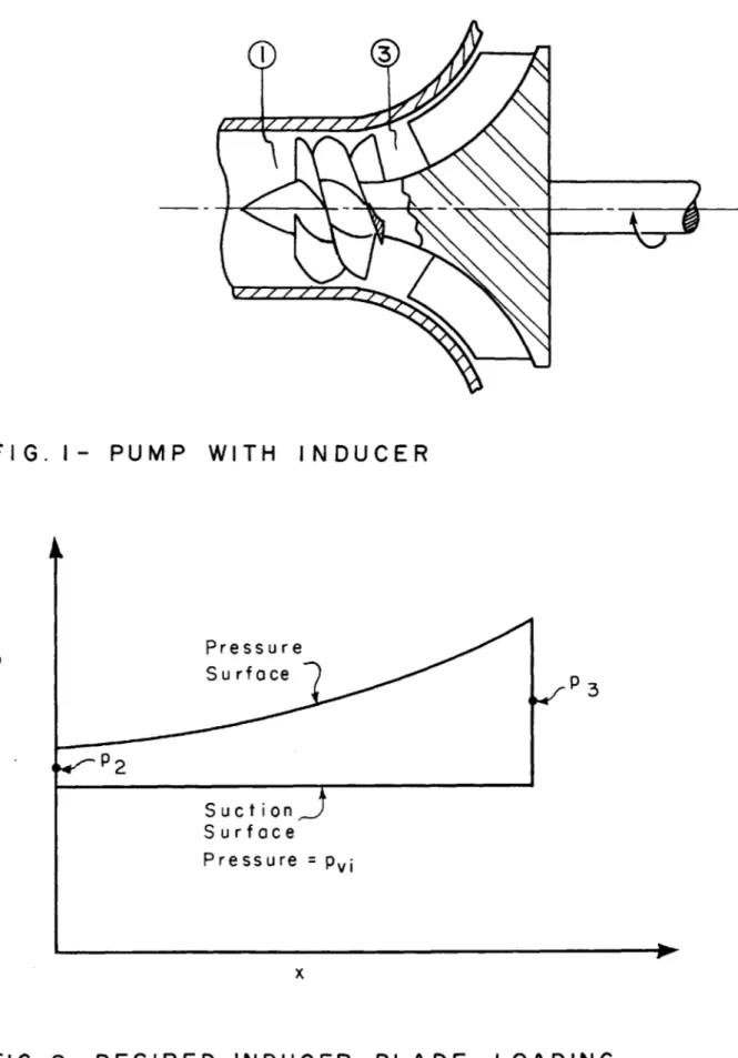
exceeds 8-10,000 (1) so that for such pumps the

maximum rotational speed without cavitation is determined by the flow and the suction head available. To permit operation at higher speeds an in-ducer or boost pump may be mounted in front of the main pump (f ig. 1). A typical axial inducer is simply a very lightly loaded axial pump which raises the pressure of the fluid sufficiently to avoid cavitation in the main pump. It has been found possible to operate inducers successfully at

su-tipn specific speeds up to 30,000, so that considerable reductions in total pump weight can be achieved when they are employed. Of course, since the inducer is simply a lightly loaded pump which is capable of handling a cavitating fluid, the functions of inducer and main pump may be combined by designing the main pump so that the inlet is lightly loaded. However,

it is not always convenient to do this and in many applications conven-tional centrifugal pumps are still used, preceded by a separate inducer.

The objective of this report is to put the design of such inducers on a rational basis by developing a method of calculating blade shapes for the optimum pressure distribution.

2 CAVITATION LIMITS

For practical purposes, cavitation may be considered to occur when the pressure falls to the vapor pressure corresponding to the inlet temperature to the inducer, that is when p = p . It is desirable to de-sign the inducer so that p does not fall below p1 at any point although

the inducer will operate satisfactorily with some cavitation. On the other hand, to make the inducer as short as possible, we should have

suc-tion surface pressures on the blading as low as efficient operasuc-tion

per-mits. A reasonable compromise between these two requirements is to de-sign for constant pressure on the suction surface, equal to the vapor pressure Pvl at the most unfavorable operating condition with respect to

cavitation (Fig, 2). Since the inducer will perform efficiently with

some cavitation a reasonable factor of safety is then included in the

de-sign.

Thus, the objective is to find the blade profile of the short-est inducer which, for a given set of inlet conditions, will produce the

required rise in pressure without severe cavitation.

To compute the maximum allowable relative velocity in the

in-ducer we assume that losses may be neglected so that the relative

stag-nation pressure is constant.

Then, at any point in the inducer

-X

where station 1 is just outside the inducer and station 2 is at the

mid-passage just inside the inducer (Fig. 3). At the point of maximum

al-lowable relative velocity (and minimum static pressure) p

=

pv and

-2--2-.

An inducer design can be carried out only if v is greater than w2 (the mid-passage velocity just inside the blading) and H sl must be suf-ficiently large to ensure that this is so.

If the inducer is operating with finite leading edge load-ing, then a9₂ C 91 0 since no change in c 9 can then occur in zero

length.

2-.

2- 2

2-W 2. (2)

From continuity

Cx

Ax

I

Cx- Ax2.

Ax-i.

where f

=

is the blockage factor of the blading. Then Ax2

HIUCRWR 2

-V++

VN 2 .. 2.

For given inlet conditions and blockage actor, the allowable

accelera-tion may be calculated. For example, with

and 01l In this case, only 1.1%

increase in velocity is allowable after the fluid enters the blading if

cavitation is to be avoided.

3

INDUJCER WORK

From the inlet conditions and the cavitation characteristics of~ the main pump, the increase in stagnation pressure to be supplied by

the inducer may be calculated as fbllows.

Let the suction specific speed of the main pump for safe

oper-ation be -. Then, from N, Q and S the necessary

head to be supplied by the inducer is equal to H - H l if the tempera-ture (and hence the vapor pressure) does not change significantly in the

inducer. For most fuels (including cryogenic fluids) the rate of change

of vapor pressure with temperature is sufficiently small to permit this

approximation. Thus,

from Euler's equation, where is the inducer efficiency, usually of the

order of

60

- 70%. With no preswirl, c

=0

0 and

from which c may be found

e LA

(6)

For a design with constant mid-passage axial velocity (such as a free

vortex design), c ' -.cx2 and (9is calculated directly from equation (6).

For designs other than free-vortex, it is necessary to compute the axial velocity distribution before (3is found. The inlet fluid angle(3,is

4 BLADE SHAPE

Inducers are sufficiently lightly loaded so that the difference between fluid angles and blade angles can be neglected for a first

approx-imation, and the blade loading can be computed by the simple one-dimen-sional approach described below. Consider the elementary control volume between two blades shown in figure 4.

Equating the tangential pressure torque on the control volume

to the net efflux of angular momentum from the control volume we have

AP,

C

where A p is the difference in pressure between the two sides of the

con-trol volume and rm, Wm are the mass-weighted mean values between the

blades which to a first approximation may be taken as the values at the

middle of the passage Vy, w4. ' is the blade-spacing.

io y

-where w is the relative velocity at mid-passage. Therefore,

If the blade loading is specified as a function of x, the allowable rate

of change of w may be calculated from equation (7).

For an inducer which is to be designed with constant suction

surface velocity equal toK W 2, where

K

and is found from the

inlet conditions, the equation becomes

or

If cx is specified as a function of x, then equation (8) may be integrated

to give as a function of x. Unfortunately, in general cx will not be

known as a function of x along a mid-passage streamline, since the radial

distribution of cx at a given x depends on the radial distribution of

(3,

as will be discussed later, yielding an exceedingly complicated

differen-tial equation for . For one simple case only (free vortex design) cx

will be constant and the equation can easily be integrated. It appears that there actually are some merits to a free vortex design for axial in-ducers, so that this sblution may be useful. The critical part of the in-ducer is the tip section and it is the blade shape at the tip which is to

be calculated. At other radial stations the suction surface pressure is

higher than at the tip and therefore the danger of cavitation is not as great.

With c constant c the equation reduces to

_Ile

2. cof

kX

Therefore

This equation integrates to

X

Cos-

OXa-

.

and requires 7 figure accuracy in the individual components to give 3

figure accuracy in the final answer for the type of machine with which we are dealing. However, if /3 is greater than 650, the assumption that

S)

:-... can be made (3 in radians) and the integral is simplified to

(10)

with negligible loss in accuracy.

For example, if

K =

1.011,

4.0,

= 1.03 then c

/c

3 *71.1I and x3

/Z

.44.

To obtain the tip coordinates of the blade, an x - 9 plot is needed, whereas equation (10) gives only x versus /3 , an inconvenient

form.

where r is the tip radius of the inducer. Therefore from equation (8)

With the approximation that

zS

(:74 ) valid for large 15

equation (11) integrates to

-

Z(12)

It is essential that the approximate expressions for x, 9 should be

con-sistent i.e. to ensure that the inducer does in fact have the desired inlet and exit angles. Equations (10) and (12) satisfy

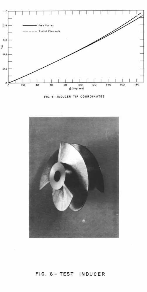
this requirement. In Figure (5) ' versus 9 is shown for the tip section

of a 3-bladed inducer with the specifications given on page (). Now

(at least for a free-vortex machine) it is possible to compute the blade coordinates for the inducer. Manufacturing considerations may dictate the use of blading other than free-vortex, in which case radial equilibrium

Even for a very lightly loaded inducer, the fluid angler will

not be exactly equal to the blade angle.6' but will in fact be greater

than

/3

'. _{The error will be on the safe side as far} as blade loading is

concerned, but if the inducer is designed with ' equal to the desired

value of

/33,

the design point work will not be attained. To remedy this,

the inducer blading should be designed for

133'

s

/33

- , where

S

is the

deviation and can be fairly accurately predicted from Carter's rule (Ref. 2),

and the computation for blade shape should be continued on to

/3

3' The

re-sulting inducer should deliver the correct work at the design point flow.

5 RADIAL EQUILIBRIUM AND THE RADIAL BLADE ELEMENT INDUCER

The example shown in Figure 5 has been worked through with the

assumption that cx is constant at the tip through the inducer. This

as-sumption is valid only if the design is free-vortex. A free-vortex

de-sign has the disadvantage of nonradial blade elements at each station, which entails some manufacturing difficulties, but the perikheral speeds are so low that no stress problems are introduced. It has the possible advantage that for a given amount of work at the tip, the static pressure leav;Lng the inducer is greater than for a forced vortex design with in-creasing work from root to tip, so that for the same amount of tip work

we might expect better cavitation characteristics from a free vortex

invariant with r at a fixed x. Therefore, at any x,

r(u

- wg) -rt(ut - wgt)

r(u

-

cxtan(3)

.rt(ut

-

cxttan(gt)

r(tan(

3₂ -

tan(3)= rt(tan( 2t

-

tan(Tt)

since ct cx -. cx2

At any (r,x), tan(

tan(2

-

F (tan9 t

-

tan(t), where("t is the tip

inducer angle at that x, and this is the equation for the blading in con-junction with the tip shape.

The most attractiye forced vortex inducer from the point of view of the machinist is one with radial blade elements i.e. one with tan

r/rt tan t at any x. Neglecting meridional streamline curvature, let us use the simple radial equilibrium equation (Ref. 3) to study the radial c distribution in an inducer of this type.

If tan(

-A

r where

4

then

k

-

k

₀

, +

- -xAS

-

kSLY-

(.-r

A~x

A Cs)

The equation reduces to

-

a

-a ?A

r

or

A

\I+rAz)cx]

-.

Therefore A IL X

₍₁₄₎

and

where rq is the reference radius where c= c .

fore, subtracting (15) from (14)

LA.

C(..

But Ar= tan/3 .

LACo

yAn(?-

C

--Solving for cx/cx2

-~~~4

173 ~

Z~4VY

But c will equal the mean value cx2 approximately halfway from

root to tip, so that tan

.J3

( ) tan/3 whereX is the ratio of hub

dia-meter to tip diadia-meter. Therefore

(16)

For an inducer with

/2t

a 75-5,

/33t -

71.f

and

X

=

0.5.

we find that

cx3t

-

1-13, representing a substantial acceleration at the tip.

(15)

There-4-r,

(v +'A'')

CCx

₊

_eAr

Alc>:

A

-(L

r5

I.-

+.. C-0 , S'

Returning to equation

(8),

in order to find the inducer blade

shape it is necessary to substitute (16) into (8) and integrate. With (16) in its exact form, the equation cannot be integrated analytically. However, a good approximation to (16) for the machines we are consider-ing is

(1 2. (17)

This expression deviates from (16) by less than 1% over the range of in-terest.

Eliminating cx between (17) and (8) and integrating with the approximation - - the equations fdr the shape4c-5(4

of the inducer are

-

-P~'(18)

-(19)

Z0-4

which reduce to (10) and (12) (as they should) when the hub-tip ratio tends to unity.

ACe

In a design problem, at the tip is known and we wish to find the outlet angle and the blade shape.

AC

U+t

CC t

=

.

C

Ac

Cx3t

Eliminating c between (17) and (20)

AC~

(I(21)

3

3 is found by a trial and error solution of (21).

x/% and 9 are then found as functions of

/3

from (18) and (19). For the example under consideration (page ') with > = 0.5, .25,

75.5 it is found that 13 is

66.2

for the radial blade element

inducer (as opposed to 71.10 for the free vortex inducer). From equation

(18) x .46 for the radial blade element inducer -- slightly longer than

the free vortex inducer. cx3t/c 2 = 1.27 for the radial element inducer.

In figure (5), the tip blade coordinates of tdhe radial element inducer are shown for purposes of comparison with the free vortex in-ducer doing the same amount of work at the tip. The difference between

fluid angle and blade angle has been neglected. With the deviation in-cluded, both inducers would be slightly longer.

6 CONCLUSIONS

An inducer design system has been developed which permits the designer to find the blading coordinates for the shortest inducer which will do the requ4red task without serious cavitation. To test the val-idity of this design system, three inducers are presently being made at the Gas Turbine Laboratory and will be tested in a pump test stand which is also under construction. These inducers have been designed for S2

"

780,

A

cot/ut = 0.20,f 1.05, X

=

0.4 and values of

K

of 1.005, 1.012 and 1.016. The corresponding values of suction specific speed at incipient cavitation are 30,000, 25,000 and 23,000, respectively. One of these in-ducers is shown in figure (6).

REFERENCES

1) Wislicenus, G. F., "Fluid Machinery", McGraw-Hill, 1947.

2) Howell, A. R., "Fluid Dynamics of Axial Compressors", The Institution

of Mechanical Engineers, Proceedings. 1945, Vol. 153.

3) Adams, H. T., "Internal Combustion Turbine Theory", Cambridge Univer-sity Press.

Ax

cx

go

HE

K

N

p Po

p

₀

Pv

P

Q

r

S

u

w

x /3 A'

cross-section area

tangential absolute velocity

axial velocity

blockage factor

A

constant in Newton's Law

suction head

maximum

velocity

ratio of

inlet velocity

rotational speed

static pressure

stagnation pressure

vapor pressure

(IL flow

radius

suction specific speed

blade speed

relative velocity

axial distance

fluid angle from axis

blade angle from axis

hub-tip ratio

inducer efficiency

rotation about x

axs

ft

2

ft/sec

ft/sec

lb.m. ft

lb.f. sec

2 ft lbs f. 1b.m.

r.p.m.

lbs

f/ft

2 lbs f/ft 2 lbs f/ft 2 g.p.m. ft ft/sec ft/sec ft

9

SUBSCRIPTS

1 before inducer 2 inside entrance

3 leaving inducer

t tip

Ak

p2

Suctio

Surface

Pressure = pvi

FIG. 2- DESIRED INDUCER

BLADE

LOADING

p

p3

@

Cx2

FIG. 3-

ENTRANCE

Control

Volume

Pressure

Wx

I

Suction

Surface

We

vW

dx

VELOCITY TRIANGLES

FIG.4 - CONTROL VOLUME

NOTATION

0

U u

'I,/

0.8 0.6 0.4 0.2 0 140 160 180

FIG. 6- TEST INDUCER

-- Free Vortex

-Radial Elements

20 40 60 80 100 120

0 (degrees)