A Deep Learning Approach to State Estimation
from Videos
by
Chandani Doshi
S.B. E.E.C.S., Massachusetts Institute of Technology, 2017 Submitted to the
Department of Electrical Engineering and Computer Science in Partial Fulfillment of the Requirements for the Degree of Master of Engineering in Electrical Engineering and Computer Science
at the
Massachusetts Institute of Technology June 2018
c
Massachusetts Institute of Technology 2018. All rights reserved.
Author . . . . Department of Electrical Engineering and Computer Science
May 11, 2018
Certified by . . . . Rebecca L. Russell Senior Member of Technical Staff, Draper Thesis Supervisor May 11, 2018 Certified by . . . . Leslie P. Kaelbling Professor of Computer Science and Engineering, MIT Thesis Co-Supervisor May 11, 2018
Accepted by . . . . Katrina LaCurts Chair, Master of Engineering Thesis Committee
A Deep Learning Approach to State Estimation from Videos
by
Chandani Doshi
Submitted to the Department of Electrical Engineering and Computer Science on May 11, 2018, in partial fulfillment of the
requirements for the degree of
Master of Engineering in Electrical Engineering and Computer Science
Abstract
Kalman filters have been commonly used for estimating the state of a vehicle from a video. Multi-State Constraint Kalman Filter (MSCKF) is an EKF-based state esti-mator that uses feature measurements for pose estimation of a vehicle. These models require a lot of hands-on engineering time to define the measurement functions. We propose a data-driven approach by training deep neural networks on high-dimensional navigation image data generated from a simulation. We describe a CNN model that robustly learns reliable features from the input and gives promising results to model temporal data. We show that a deep learning approach can be a replacement for the MSCKF model for estimating the velocity of a moving vehicle.
Thesis Supervisor: Rebecca L. Russell
Title: Senior Member of Technical Staff, Draper Thesis Supervisor: Leslie P. Kaelbling
Acknowledgments
I would like to thank Rebecca L. Russell and Abraham R. Schneider, my supervisors at Draper for their continued support. Their guidance helped me throughout the research and writing of this thesis.
I would like to acknowledge Professor Leslie P. Kaelbling at MIT as my thesis co-supervisor. I am grateful for her comments on this thesis. Working with each of my supervisors was a great learning experience.
Contents
1 Introduction 13
2 Prior Work 17
2.1 Kalman Filter . . . 17
2.1.1 Deep Kalman Filter . . . 18
2.2 Neural Networks . . . 18
3 Model 21 3.1 Background . . . 21
3.1.1 Feedforward neural networks . . . 21
3.1.2 CNN . . . 22
3.1.3 RNN . . . 23
3.2 3D Convolutional Neural Network . . . 24
3.3 RNN Model . . . 26
3.4 Learning . . . 26
4 Data Collection 29 5 Experimentation 33 5.1 Preliminary Training . . . 33
5.2 New Validation Set . . . 37
5.3 Data Augmentation . . . 37
5.4 Reducing size of CNN . . . 39
List of Figures
2-1 Graphical representations of Kalman filter and RNN model . . . 19
3-1 Architecture of a feedforward neural network . . . 22
3-2 A typical CNN architecture. Source [2] . . . 22
3-3 RNN architectures . . . 24
3-4 CNN architecture . . . 25
3-5 RNN architecture . . . 27
4-1 Aerial view of the environment developed in Unreal Engine . . . 30
4-2 Different datasets generated from Unreal Engine simulation . . . 31
5-1 Plot of true and predicted speeds over time . . . 34
5-2 Graph of predicted speed vs true speed . . . 35
5-3 Visualization of features learnt using the CNN model on the dataset containing dashed lines . . . 36
5-4 Visualization of features learned using the CNN model on the dataset containing solid line . . . 38
5-5 Modified CNN architecture . . . 40
5-6 Plot of true and predicted speeds over time . . . 41
List of Tables
5.1 CNN Performance . . . 34 5.2 RNN Performance . . . 39
Chapter 1
Introduction
State estimation of a moving object has received considerable attention in the research community. Vision-aided inertial navigation uses data from a camera and an Inertial Measurement Unit (IMU) to track the position and orientation of a moving vehicle and estimate its motion. Kalman filters have been commonly used to estimate an object’s location based on multiple observations over time. A Kalman filter provides a recursive solution to estimate the current state of an object based on its previous state and the new input data.
In classical Kalman filters [13], the latent state evolution as well as the emission distribution and action effects are modeled as linear functions perturbed by Gaussian noise. The Extended Kalman Filter (EKF) [30] [25] and the Unscented Kalman Filter [33] are extensions to the classical Kalman filter that can be used for nonlinear estimation. Using Kalman filters and traditional computer vision approaches, we can build a model that learns the state of a moving vehicle from a contiguous sequence of images.
Traditional computer vision techniques can extract multiple features such as edges, corners, etc. from images, which are high-dimensional, information-rich measure-ments. When using navigation data, some challenges to Kalman filters and tradi-tional computer vision approaches are lighting, traffic, homogeneous environments (long stretches of fields), etc. Accounting for each of the challenges requires modifi-cation of the system, adding and removing different types of sensors, thus, having a
high cost to change. Being able to handle a large rate of high-dimensional data limits the algorithmic complexity.
The Multi-State Constraint Kalman Filter (MSCKF) was introduced by Mourikis and Roumeliotis [21] for real-time vision-aided inertial navigation. This method is able to optimally utilize the localization information provided by multiple measure-ments of visual features. The authors introduce a measurement model that expresses geometric constraints between camera poses, allowing it to estimate the pose and motion of a vehicle. However, feature measurement for this model requires hands-on engineering time to update and define the measurement functions.
We seek to model a state estimator that can learn from a time sequence of images generated from a video to estimate motion of a vehicle, and is comparable to the MSCKF model. We propose to model the change of pose of a vehicle over time using deep neural networks. Neural networks approximate a mapping function from input variables to output variables. They are robust to noise in the input data, and can support learning and prediction in the presence of missing values. Neural networks can approximate nonlinear functions making them valuable in time series processing [3].
Convolutional neural networks (CNNs) have led to impressive results in object recognition [17], face verification [24], and audio classification [19]. A CNN consists of a sequence of convolutional layers that produce an output by sliding a filter (a matrix of weights) over the input, and computing the dot product between the two. The convolutional layer allows the model to learn filters that can extract features or patterns from the input data. Bikowski et al. describe an autoregressive-like weighting system for time series forecasting, where the weights are data-dependent functions learnt through the network [1]. The idea behind using a CNN to model a moving vehicle would be to learn filters representing patterns in the series of images that can be used to predict the velocity of the vehicle.
Recurrent neural networks (RNNs) are being used to model time sequences [5] [8]. RNNs and long short term memory (LSTM) networks, a variant of RNN, can be used for time series predictions [20] [7]. This network architecture has shown
improved performance over Hidden Markov Models in long-term context tasks such as speech recognition [26]. The success of the recurrent network model lies in its recurrent connections that allow the network to use the entire history of time series values while predicting the value of the next time step.
In this paper, we describe two models involving a convolutional neural network and a recurrent neural network to model the contiguous sequence of frames generated from a video. We show that these networks are able to learn to estimate the motion of a vehicle and that to do so, the networks learn reliable features that are useful for decoding the state of an object.
Chapter 2
Prior Work
2.1
Kalman Filter
The Kalman filter provides a recursive solution to the linear optimal filter problem. The solution is recursive as each updated estimate of the state is computed from the previous estimate and the new input data.
Assume we have a set of unknown state vectors x1, . . . , xT. For each unobserved
variable xt, we have a corresponding observation zt. The Kalman filter model assumes
that the true state at time t evolves from the state at t − 1 according to:
xt= Ftxt−1+ wk
where Ftis the state transition matrix and wt∼ N (0, Qt) is the process noise, which
is a zero-mean Gaussian distribution with covariance Qt. At time t, the filter models an observation zt as follows:
zt= Htxt+ vt
where Htis the observation matrix, which maps the true state space into the observed
space, and vt ∼ N (0, Rt) is the observation noise, which is a zero mean Gaussian
white noise with covariance Rt.
architecture that includes a gain function and a recursive step. While modeling object tracking for a moving vehicle, the gain function has to be modified to capture different conditions. This can prove to be tedious. For example, if we only the front sensors to capture the state of a car while driving through a tunnel, there will be a sudden change in the lighting contrast on reaching the end of the tunnel. In such a case, additional sensors placed at other places on the car would provide better state data. So we would have to model our gain function to be able to adapt to these changes. Similarly, when moving through traffic, it is difficult to predict all the different situations that can be faced. This is why there is a high cost to change when using Kalman filters.
2.1.1
Deep Kalman Filter
Krishnan et al. describe a method to learn Kalman filters using neural networks in [16]. The authors propose a method for learning causal generative temporal models from high-dimensional data, using deep neural networks as a building block. The model fits a generative model to a sequence of observations and actions. The obser-vations come from a latent state which evolves over time, and the authors assume the observations to be a noisy, nonlinear function of this latent state. The latent states are nonlinear functions of the previous latent state and the previous actions. These nonlinear functions are parameterized using MultiLayer Perceptrons and Recurrent Neural Networks, allowing the model to learn a broad range of Kalman filters. Using this model, the authors get promising results to show that the parametric posterior learnt can be used to approximate the latent state of unseen data.
2.2
Neural Networks
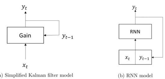
Deep neural networks allow us to build data-driven models that learn features and a gain function. Multilayer feedforward networks can be used for universal function approximation [11]. They can learn linear and nonlinear relationships when learning a mapping function using the inputs. As shown in Figure 2-1b, a recurrent neural network has a loop that allows information to persist. The ability of recurrent neural
(a) Simplified Kalman filter model (b) RNN model
Figure 2-1: Graphical representations of Kalman filter and RNN model
networks to learn the temporal dependence in the input data can be used to capture state in a time series.
The success of the convolutional neural network in image analysis tasks lies in its ability to learn complex feature representations through the convolutional layers. As mentioned before, the authors of [1] propose to use a convolutional network in-volving an autoregressive-type weighting system to forecast time series. Gregor et al. introduce an autoregressive network that is a deep, generative autoencoder [9]. This network is a universal distribution approximator, capable of capturing high-level structure in data. The autoregressive structure captures dependence among units within the same layer and from the previous layer. Using autoencoders, the model learns to encode and decode observations according to a compression metric yielding concise, meaningful representations.
PixelCNN [32] proposed by Oord et al. builds on the idea of autoregressive net-works. It consists of stacked masked convolutional layers that allow the predictions for all pixels to be made in parallel during training. During sampling, every time a pixel is predicted, it is fed back into the network to predict the next pixel. The masking forces the model to learn to predict each pixel based on previous inputs. Oord et al. introduce WaveNet [31], a model based on the PixelCNN. WaveNet is a generative model that operates on the raw audio waveform. Similar to PixelCNN, this network models conditional probability using a stack of convolutional layers. The
combination of causal filters with dilated convolutions allows the receptive fields to grow exponentially with depth, thus allowing the network to model long-range tempo-ral dependencies in audio signals. WaveNets have shown promising results in speech recognition tasks.
FlowNet proposed by Fischer et al. [6] uses convolutional networks to learn pre-dicting the optical flow field from a pair of images. Optical flow is the pattern of apparent motion of objects in a visual scene caused by the relative motion between an observer and a scene. Optical flow estimation needs precise per-pixel localization, and requires finding correspondences between two input images. The authors show that it is possible to use CNNs to learn image feature representations and match them at different locations in the two input images.
Chapter 3
Model
In this section, we start with a review of neural networks and then discuss the par-ticular deep learning model architectures developed for state estimation. We focused on two neural network models: convolutional neural networks and recurrent neural networks. As discussed in the previous chapter, both of these models have shown significant results in time series predictions. We define two models that learn mean-ingful features from the continuous stream of frames of a navigation video generated using a simulator which is further discussed in Chapter 4. The first model is based on a CNN and the second model uses a combination of convolutional layers and a RNN. The ability to learn a gain function from the data gives this deep learning approach an advantage over Kalman filters, where we would have to manually modify the gain function.
3.1
Background
3.1.1
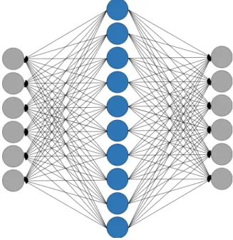
Feedforward neural networks
A feedforward neural network receives an input and transforms it through a series of hidden layers. Each hidden layer consists of a set of nodes or neurons, where each node is fully connected to all nodes in the previous layers. Each node is a weighted sum of the nodes of the previous layer followed by a bias offset. We use nonlinear
activation functions to model nonlinearity in the data.
Figure 3-1: Architecture of a feedforward neural network
3.1.2
CNN
In a simple convolutional neural network, the input is passed through a series of convolutional layers, nonlinear layers such as Rectified Linear Units (ReLU), pooling layers, and fully-connected layers. Figure 3-2 shows the architecture of a standard CNN.
Figure 3-2: A typical CNN architecture. Source [2]
neuron to each output neuron in the next layer, as is done in a feedforward neural network, we use convolutions over the input layer to compute the output in a CNN. This means that a neuron in the output layer is only connected to a set of neurons in the input layer, resulting in local connections. The convolution layer extracts specific patterns from the input data using a filter, which is a matrix of weights. The filter slides over the input, computing element-wise multiplications. The multiplications are then summed up and the process is repeated by moving the filter to the right on the input, creating a feature map. The stride and filter size determine the overlap in the regions connecting to the output nodes. Having multiple layers of convolution allows the network to learn high-level filters with relatively fewer parameters. The feature map produced by the convolution layer is passed through ReLU, a commonly used nonlinear activation function which replaces all negative value in the feature map by zero. The pooling layer reduces the spatial size of the representation and controls overfitting by reducing the amount of parameters and computation in the network. The fully connected layers are the same as a feedforward network and perform classification on the feature map extracted by the convolutional layer and down-sampled by the pooling layer.
3.1.3
RNN
The simple RNN architecture proposed by Elman [5] can only retain short term con-text due to the vanishing gradients problem. The weights of the neural network are updated proportional to the gradient of the error function with respect to the current weight in each iteration of training. The gradients decay exponentially, preventing the weights from changing. This means that, over time, the influence of the past in-puts decays quickly. The architecture of the Elman RNN can be seen in Figure 3-3a. To overcome the problem of vanishing gradients, we use a variation of RNN architec-ture called LSTM, Long Short Term Memory. LSTM networks were introduced by Hochreiter and Schmidhuber [10] and are capable of learning long-term dependencies. An LSTM block (Figure 3-3b) is composed of four main components: a cell state, an input gate, an output gate, and a forget gate. The gates act as regulators of the
flow of information that goes through the connections of the LSTM and can, thus, control the cell state. These gates allow the cell state to remember information over arbitrary time intervals.
(a) Elman RNN architecture (b) LSTM block [22]
Figure 3-3: RNN architectures
3.2
3D Convolutional Neural Network
Networks built for image recognition applications generally use 2-dimensional CNNs [18] [27]. In 2D CNNs, convolutions are applied on the 2D feature maps to compute features from the spatial dimensions only. When analyzing videos, we want the network to capture motion information encoded in multiple contiguous frames. To fuse information across the temporal dimension, we use 3D convolutions to compute features from both the spatial and temporal dimensions. This approach of using 3-dimensional spatiotemporal convolutions has been used for human action recognition from videos in [12] and for large-scale video classification in [14] and [28]. For a 3D convolution, we stack the contiguous sequence of frames together and convolve a 3D kernel across this stack. Since the feature maps in the convolution layer are connected to multiple contiguous frames in the previous layer, this method can capture motion information.
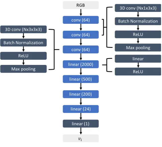
Using a combination of 2D and 3D convolutions, we devised a CNN architecture, shown in Figure 3-4 to estimate the state of a moving vehicle from videos. The network consists of a series of convolution modules to learn feature representations
Figure 3-4: CNN architecture
from the input, followed by fully-connected modules for estimation. Each convolution module consists of a convolution layer with 64 filters, a batch normalization layer, and a nonlinear ReLU activation layer. The fully-connected modules consist of a linear layer and a ReLU layer. The first two layers apply 3D convolutions with a kernel size of 1 × 3 × 3, with 1 in the temporal dimension and 3 × 3 in the spatial dimensions, so these are essentially 2D convolutions. We use max pooling with a kernel size of 1 × 3 × 3 and stride 2. The initial convolutional layers extract features such as edges from the input images. We modify the last layer of convolutional filters to extend in time by using a 3D spatiotemporal convolution with a kernel size of 3 × 3 × 3 (with 3 in the temporal dimension and 3 × 3 in the spatial dimension) and apply max pooling
with kernel size 3 × 3 × 3 and stride 2. This layer maps features that are reliable to capture motion over time. The output of the final convolution module is passed through the fully-connected layers. Figure 3-4 uses linear(n) to represent a linear layer with n nodes.
We use a sliding window approach when passing in multiple contiguous frames to the network and return the estimated velocity for the middle value of the window.
3.3
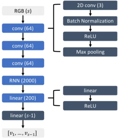
RNN Model
The RNN model is diagrammed in Figure 3-5. We use a series of 2D convolution modules consisting of 2D covolution layers, batch normalization, ReLU activations and max pooling, followed by fully-connected modules consisting of linear layers and ReLU activations. We start by applying 2D convolutions with 64 filters and kernel size of 3 to process the contiguous sequence of frames and extract features. We stack the color channels for all frames in the sequence at each time step and perform the convolution over this stack, thus, convolving the filter only over the spatial dimensions. We use max pooling with a kernel size of 2 and stride 2. The feature map produced is passed into a RNN with 200 features in the hidden state. The output of the RNN is fed into the fully-connected layers. The output of the final linear layer returns the predicted velocity between each pair of contiguous frames in the sequence. So, for a given sequence of s contiguous frames, the final output will contain s − 1 values of estimated velocities.
3.4
Learning
We use the Adam [15] optimizer with a learning rate of 0.001 to train our CNN model. We use the Adamax algorithm [15] with a learning rate of 0.01 to optimize our RNN model. Both models use a batch size of 64 and the mean squared error loss function.
Chapter 4
Data Collection
To gain an understanding of the representations learned in the proposed frameworks, we trained our models on synthetic data. We wanted data that captures all scenarios that pose a challenge to object tracking. The model has to be robust to handle varied lighting conditions and homogeneous features such as long stretches of fields. Using real vehicles to obtain this data would be expensive. There is a high cost to change such as adding new sensors. To overcome this challenge, we built a simulation for which we have access to the underlying generative model and all latent parameters, thus, making our dataset easily modifiable. One example of such a simulation is CARLA [4], an open-source simulator for autonomous driving research. Using a simulation allows us to examine whether our models can be used for the defined purpose, without incurring the high cost of gathering data in the real world.
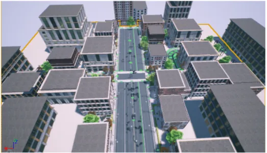
We developed a simulator that mimics real-world driving scenarios. The simulator is built using Unreal Engine, a game development environment. Using the Urban City [23] package, we have built the layout of a city. Figure 4-1 shows an aerial view of the system. Unreal Engine allows for easy modification, thus, reducing the cost of making changes. The simulation has a car moving forward with randomly-varying smooth acceleration, allowing the simulation to capture a large variety of speed changes throughout the course. The environment is easily modifiable to account for lighting conditions at different times of a day. We use a Python plugin for Unreal Engine [29] to simulate the motion of a car and capture frames. For each frame, we
store the time, and the position and orientation of the vehicle. This allows us to calculate the velocity between subsequent frames.
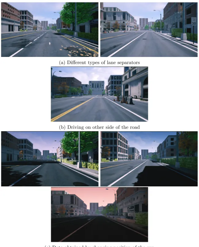
Some examples of the types of images captured from this simulation can be seen in Figure 4-2. We generated datasets by developing an initial environment, modifying the order and type of buildings from the initial environment, driving in the opposite direction on the other side of the road, and changing the time of day to change the position of the sun. As the generated images have a high resolution, we train the networks with images of lower resolution.
(a) Different types of lane separators
(b) Driving on other side of the road
(c) Data obtained by changing position of the sun
Chapter 5
Experimentation
We compare the performance of our models to an implementation of MSCKF [21]. As mentioned in Chapter 1, MSCKF is an EKF-based vision-aided inertial navigation system that can estimate pose from video and IMU data. The IMU measurements received are processed for propagating the EKF state and covariance. For each new image that is recorded, the current camera pose estimate is augmented to a state vector. While updating the EKF, the measurements of each tracked feature are employed for imposing constraints between all camera poses from which the feature was seen. So state augmentation is necessary for processing feature measurements. The EKF vector, thus, comprises of the changing IMU state and a history of the past poses of the camera, allowing this measurement model to estimate the pose and motion of a vehicle.
The MSCKF model used for comparison was developed for real-world data and was not heavily tuned on the simulation. We report prediction error as the average of the absolute difference between the predicted and true speeds. The accuracy is calculated using the relative error between the predicted and true speeds.
5.1
Preliminary Training
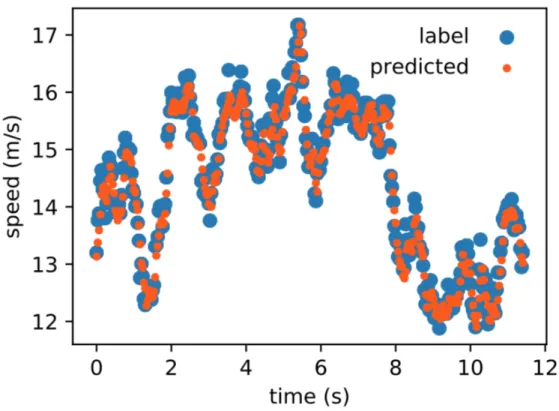
First, we trained the CNN model described in Section 3.2 with the dataset containing dashed lane separators 4-2a. As can be seen in Table 5.1, the average error of the
Figure 5-1: Plot of true and predicted speeds over time
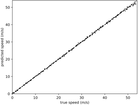
CNN model is much lower than that of the MSCKF model. Figure 5-1 shows the true and predicted speeds in one run of the validation set. As can be seen in the figure, the network is able to predict the speeds of the vehicle in a pattern which is similar to that of the true speeds, but is less noisy. This shows that the network is learning reliable feature representations for state estimation and is robust to noise. Figure 5-2 is graphed using a subset of speeds in the dataset, and shows that during prediction at higher speeds, the network underestimates the speed.
MSCKF CNN CNN CNN Small CNN
(dashed line) (solid line) (data aug) (data aug)
Error (m/s) 0.9301 0.15 1.64 1.19 1.04
Table 5.1: CNN Performance
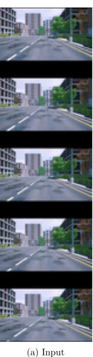
Figure 5-3 shows a sequence of images passed to the model as input and the features learnt by the model obtained by performing guided backpropagation.
Visu-Figure 5-2: Graph of predicted speed vs true speed
alizing the part of an image that most activates a given neuron using backpropagation is a method using a backward pass of the activation of a single neuron after a forward pass through the network and, computing the gradient of the activation with respect to the image. While propagating the gradient through the nonlinear layer ReLU dur-ing guided backpropagation [27], we clip the negative gradients to zero, preventdur-ing the backward flow of negative gradients corresponding to neurons that decrease the activation of the higher layer unit we aim to visualize. Doing so allows us to see the image features the model detects and not the stuff it does not detect.
As can be seen in Figure 5-3b, the main feature learnt in this experiment is the dashed line on the road. This makes sense because the dashed lines are present at regularly spaced intervals and are a good indicator of the speed of the car. We want to see whether our network is robust to different environments where such easily identifiable, periodic features are not present. So, for the subsequent experiments, we
(a) Input (b) Guided backpropagation
Figure 5-3: Visualization of features learnt using the CNN model on the dataset containing dashed lines
modified the environment by replacing the dashed lane separators with a solid line.
5.2
New Validation Set
For the preliminary evaluation, we generated the training and validation sets from the same dataset. This can lead to the network overfitting to the input dataset. To prevent overfitting, we developed a different environment that is used as a validation set. We wanted to ensure that the network does not learn the order of the buildings in the environment, so we changed the order and type of buildings used.
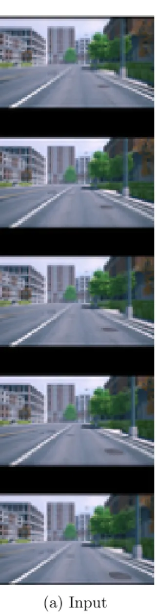
Table 5.1 shows the validation performance of the CNN model using the new validation and training sets. The highest accuracy achieved by the CNN model is around 84.27% with an average error of 1.64 m/s which is much higher than the error obtained by training the model on the old dataset. This makes sense because the network can no longer learn the regularly spaced dashed lines and the validation dataset is different from the training dataset, so the network does not overfit to a particular environment. As can be seen in Figure 5-4, the network learns a set of features that are present in the given set of contiguous frames. In this example, one of the features learnt is the base of the streetlight. This feature is present in each frame, and the change in position of this feature provides an estimate for the motion of the vehicle. Therefore, the network robustly adapts to learn different features for each frame and for a given set of contiguous frames, using the common features of the set, the network can accumulate motion information for state estimation.
5.3
Data Augmentation
We take advantage of data augmentation to reduce the effects of overfitting by training the CNN on the original dataset along with multiple variations of the simulation as shown in Figure 4-2b and Figure 4-2c. The best performing model has an accuracy of 87.06% with an average error of 1.19 m/s as mentioned in Table 5.1.
(a) Input (b) Guided backpropagation
Figure 5-4: Visualization of features learned using the CNN model on the dataset containing solid line
be seen in Table 5.2. We obtained an average error of 2.63 m/s and an accuracy of 72.1% using the RNN architecture. We require extensive hyperparameter tuning of this model to evaluate its performance.
MSCKF RNN
(data augmentation)
Error (m/s) 0.9301 2.63
Table 5.2: RNN Performance
5.4
Reducing size of CNN
To speed up and tune the performance of the network, we reduce the number of layers and the number of neurons in each layer. The new architecture can be seen in Figure 5-5. We found that reducing the size of the network and training it on the augmented dataset improved the performance. As seen in Table 5.1, the best performing model using this architecture has an average error of 1.04 m/s with an accuracy of 89%. This error is comparable to that of the MSCKF model (0.903 m/s), showing that it is possible to use the CNN as a replacement for the MSCKF approach to predict velocity.
Figure 5-6 shows that the network still captures the pattern of speeds observed during one run through the course. Figure 5-7 represents the error obtained for a sample of speeds in the dataset, and as can be seen in the plot, there is much higher error at a higher speed.
5.5
Hyperparameter Tuning
We performed some hyperparameter tuning for both network architectures by training multiple models and choosing the model with the best performance. The tuned hyperparameters include the learning rate, the batch size, and the size of the kernels in the convolutional layers. The optimal hyperparameters found are mentioned in the
Figure 5-5: Modified CNN architecture
network architectures shown in Figure 5-5 and Figure 3-5.
It would be useful to perform a more extensive search across more of the net-works’ hyperparameters especially for the RNN model. Some of the hyperparameters that can be tuned are the weight decay, dropout probabilities, number of filters in convolutional layers, and number of filters in the hidden state of the RNN.
Chapter 6
Conclusion
The convolutional neural network developed shows promising results to model tempo-ral data generated from videos. When the data contained dashed lane separators, the network outperformed the MSCKF. But, when the data contained a solid lane sepa-rators, the model achieved results comparable to those estimated from the MSCKF. The feature visualizations show that the network is able to robustly learn internal rep-resentations that are reliable for estimating the pose of the vehicle. This shows that this convolutional neural network model can be used as a replacement for Kalman filters to calculate the velocity of a moving object when there are large amounts of high-dimensional data. Using a model that can learn from data has an advantage over Kalman filters in requiring less hands-on time to engineer the gain functions. Having a comparable deep learning solution that only requires video data is advan-tageous because MSCKF requires both video and IMU data to model camera poses and estimate velocity.
Future work involves extensively tuning the RNN architecture, and augmenting the RNN model with 3-dimensional convolutions. Due to its ability to retain long-term dependencies in data, we can examine the possibility of the RNN model being a replacement for Kalman filters in terms of being able to learn the pose, orientation, and velocity of a moving vehicle. We will also develop a simulation that permits lateral motion of the vehicle to evaluate whether our networks can estimate velocities in different directions and will add complexity to the simulation by adding features
Bibliography
[1] Mikolaj Binkowski, Gautier Marti, and Philippe Donnat. Autoregressive convo-lutional neural networks for asynchronous time series. CoRR, abs/1703.04122, 2017.
[2] Denny Britz. Understanding convolutional neural networks for NLP. WILDML. [3] Georg Dorffner. Neural networks for time series processing. Neural Network
World, 6:447–468, 1996.
[4] Alexey Dosovitskiy, German Ros, Felipe Codevilla, Antonio Lopez, and Vladlen Koltun. CARLA: An open urban driving simulator. pages 1–16, 2017.
[5] Jeffrey L. Elman. Finding structure in time. Cognitive Science, 14:179–211, 1990.
[6] Philipp Fischer, Alexey Dosovitskiy, Eddy Ilg, Philip H¨ausser, Caner Hazir-bas, Vladimir Golkov, Patrick van der Smagt, Daniel Cremers, and Thomas Brox. FlowNet: Learning optical flow with convolutional networks. CoRR, abs/1504.06852, 2015.
[7] Felix A. Gers, Douglas Eck, and J¨urgen Schmidhuber. Applying LSTM to time series predictable through time-window approaches. pages 193–200, 2002. [8] C. Lee Giles, Steve Lawrence, and Ah Chung Tsoi. Noisy time series prediction
using recurrent neural networks and grammatical inference. Machine Learning, 44(1):161–183, Jul 2001.
[9] Karol Gregor, Andriy Mnih, and Daan Wierstra. Deep autoregressive networks. CoRR, abs/1310.8499, 2013.
[10] Sepp Hochreiter and Jrgen Schmidhuber. Long Short-Term Memory. 9:1735–80, 12 1997.
[11] Kurt Hornik, Maxwell Stinchcombe, and Halber White. Multilayer feedforward networks are universal approximators. Neural Networks, 2:359–366, 1989. [12] S. Ji, W. Xu, M. Yang, and K. Yu. 3D convolutional neural networks for
hu-man action recognition. IEEE Transactions on Pattern Analysis and Machine Intelligence, 35(1):221–231, Jan 2013.
[13] Rudolph Emil. Kalman. A new approach to linear filtering and prediction prob-lems. Journal of Fluids Engineering, 82(1):35–45, 1960.
[14] A. Karpathy, G. Toderici, S. Shetty, T. Leung, R. Sukthankar, and L. Fei-Fei. Large-scale video classification with convolutional neural networks. In 2014 IEEE Conference on Computer Vision and Pattern Recognition, pages 1725–1732, June 2014.
[15] Diederik P. Kingma and Jimmy Ba. Adam: A method for stochastic optimiza-tion. CoRR, abs/1412.6980, 2014.
[16] Rahul G. Krishnan, Uri Shalit, and David Sontag. Deep Kalman filters. 2015. [17] Alex Krizhevsky, Ilya Sutskever, and Geoffrey E. Hinton. ImageNet classification
with deep convolutional neural networks. Commun. ACM, 60(6):84–90, May 2017.
[18] Yann LeCun, Bernhard E. Boser, John S. Denker, Donnie Henderson, R. E. Howard, Wayne E. Hubbard, and Lawrence D. Jackel. Handwritten digit recog-nition with a back-propagation network. In D. S. Touretzky, editor, Advances in Neural Information Processing Systems 2, pages 396–404. Morgan-Kaufmann, 1990.
[19] Honglak Lee, Yan Largman, Peter Pham, and Andrew Y. Ng. Unsupervised feature learning for audio classification using convolutional deep belief networks. In Proceedings of the 22nd International Conference on Neural Information Pro-cessing Systems, NIPS’09, pages 1096–1104, USA, 2009. Curran Associates Inc. [20] Pankaj Malhotra, Lovekesh Vig, Gautam Shroff, and Puneet Agarwal. Long
short term memory networks for anomaly detection in time series. 04 2015. [21] Anastasios I. Mourikis and Stergios I. Roumeliotis. A multi-state constraint
Kalman filter for vision-aided inertial navigation. Proceedings of IEEE Interna-tional Conference on Robotics and Automation, pages 3565–3572, 2007.
[22] Christopher Olah. Understanding LSTM networks, 2015. [23] PolyPixel. Urban city.
[24] Florian Schroff, Dmitry Kalenichenko, and James Philbin. Facenet: A unified embedding for face recognition and clustering. CoRR, abs/1503.03832, 2015. [25] D. Simon. Kalman filtering with state constraints: A survey of linear and
non-linear algorithms. IET Control Theory Applications, 4(8):1303–1318, August 2010.
[26] Hagen Soltau, Hank Liao, and Hasim Sak. Neural speech recognizer: Acoustic-to-word LSTM model for large vocabulary speech recognition. CoRR, abs/1610.09975, 2016.
[27] Jost Tobias Springenberg, Alexey Dosovitskiy, Thomas Brox, and Martin A. Riedmiller. Striving for simplicity: The all convolutional net. CoRR, abs/1412.6806, 2014.
[28] Du Tran, Lubomir D. Bourdev, Rob Fergus, Lorenzo Torresani, and Manohar Paluri. C3D: Generic features for video analysis. CoRR, abs/1412.0767, 2014. [29] twentytab. UnrealEnginePython.
[30] J. K. Uhlmann. Algorithms for multiple target tracking. American Scientist, 80(2):128–141, 1992.
[31] A¨aron van den Oord, Sander Dieleman, Heiga Zen, Karen Simonyan, Oriol Vinyals, Alex Graves, Nal Kalchbrenner, Andrew W. Senior, and Koray Kavukcuoglu. Wavenet: A generative model for raw audio. CoRR, abs/1609.03499, 2016.
[32] A¨aron van den Oord, Nal Kalchbrenner, Oriol Vinyals, Lasse Espeholt, Alex Graves, and Koray Kavukcuoglu. Conditional image generation with PixelCNN decoders. CoRR, abs/1606.05328, 2016.
[33] Eric A. Wan and Rudolph van der Merwe. The unscented Kalman filter for nonlinear estimation.