Design and analysis of MEMS-based metamaterials

(1)

Design and Analysis of MEMS-Based

Metamaterials

by

Jonathan S. Varsanik

Submitted to the Department of Electrical Engineering and Computer Science

in partial fulfillment of the requirements for the degree of

Master of Engineering in Electrical Engineering and Computer Science at the

MASSACHUSETTS INSTITUTE OF TECHNOLOGY

June 2006

©

The author hereby grants to MIT permission to reproduce and distribute publicly paper and electronic copies of this thesis document

in whole or in part.

A uthor ... ...

Department !ot Electrical Engineering and Computer Science May 26, 2006 Certified by ... Amy Duwel Charlpq q1-crL T-'-m-- T m ,---- Supervisor Certified by ... .. ... i-Au Kong 3upervisor Accepted by.... ... C. Smith

Chairman, Department Committee on Graduate Students

MASSACHUSETTS INSTiJTE

OF TECHNOLOGY

(2)

(3)

Design and Analysis of MEMS-Based Metamaterials

by

Jonathan S. Varsanik

Submitted to the Department of Electrical Engineering and Computer Science on May 26, 2006, in partial fulfillment of the

requirements for the degree of

Master of Engineering in Electrical Engineering and Computer Science

Abstract

Metamaterials, materials that are constructed with arrays of small elements have sig-nificant potential to provide material properties that are useful for electromagnetic applications but are not found in nature. Slight changes to a repeated unit cell can be used to tune the effective bulk material properties of a metamaterial, replacing the need to discover suitable materials for an application with the ability to design a structure for the desired effect. However, most current metamaterial realizations are plagued by high loss, large size, awkward structure, or difficult construction. The use of Micro-Electro-Mechanical Systems (MEMS) to create a new metamaterial could

improve upon some of these shortcomings due to their small size, high

Q,

and ease

of integration into standard applications and circuit fabrication techniques. In this thesis, I analyze the prospects of a MEMS-based metamaterial. First, I determine the best type of MEMS resonator to use in a metamaterial. Then, I build models that can accurately describe a metamaterial constructed of MEMS unit cells. Analysis of these models provides information about the potential behavior of a MEMS metama-terial. It is discovered that it is possible to create a left-handed metamaterial using

MEMS resonators. Finally, phase-shifting and antenna miniturization applications

are suggested as potential areas that can leverage the benefits of this new MEMS metamaterial.

Charles Stark Draper Laboratory Thesis Supervisor: Amy Duwel M.I.T. Thesis Supervisor: Jin-Au Kong

(4)

(5)

Acknowledgments

I would like to thank my Draper Supervisor, Dr. Amy Duwel for all her help

through-out the entire year. Also at Draper, James Kang, James Hsiao, John Lachapelle, and Doug White, all had knowledge to offer in the course of this thesis. At MIT, my Thesis Advisor, Professor Jin Au Kong, along with Dr. Bae-Ian Wu provided a great wealth of knowledge in the area of metamaterials and electromagnetics that I wish I had given more consultation.

Personally, I would like to thank my girlfriend Catherine for making sure that I ate well, my mother for putting up with me, and my father for looking over me.

Thank you all.

This thesis was prepared at The Charles Stark Draper Laboratory, Inc., under In-ternal Company Sponsored Research and Development Project 20301-001, Miniature Antenna Technology.

Publication of this thesis does not constitute approval by Draper of the findings or conclusions contained herein. It is published for the exchange and stimulation of ideas.

(6)

THIS PAGE INTENTIONALLY LEFT BLANK

(7)

5 Conclusion 5.1 _{Future W ork . . . .} 8 . . . . 5 3 . . . . 5 3 . . . . 5 5 . . . . 5 6 . . . . 5 6 . . . . 5 8 . . . . 6 1 . . . . 6 1 . . . . 6 1 . . . . 6 4 . . . . 6 5 . . . . 6 5 . . . . 67 erial 69 . . . . 70 . . . . 72 . . . . 72 . . . . 76 . . . . 77 . . . . 77 . . . . 80 . . . . 8 1 . . . . 86 . . . . 86 . . . . 88 89 93 94 53

(9)

5.1.1 Problems to Address . . . . 95 5.1.2 Applications to Consider . . . . 95

A Mathematical Work 97

A.1 Calculating the Impedance of a Coplanar Transmission Line . . . . . 97 A.2 Calculating the Torque on a Cantilever . . . . 100

(10)

(11)

List of Figures

1-1 2D rod and split ring resonator metamaterial. Taken from

[34]

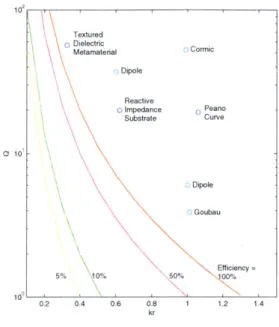
. . . . 22

1-2 Plot of the Chu limit for various efficiencies and antennas. . . . . 25

1-3 Three metamaterial antenna applications . . . . 26

2-1 A MEMS paddle resonator with the dimensions labeled. From

[9]

. . 30

2-2 Three-dimensional model of the paddle resonator with lumped circuit elem ents labeled. . . . . 31

2-3 Broadband equivalent circuit model of the paddle resonator . . . . 33

2-4 A force diagram for one side of the paddle resonator. . . . . 38

2-5 Impedance of the paddle resonator. . . . . 42

2-6 Closer view of resonance of impedance of the paddle resonator. ... 43

2-7 Signal through the paddle resonator. (dB) . . . . 43

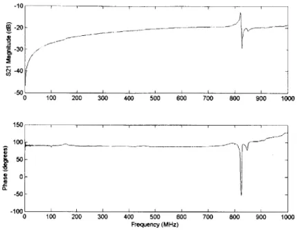
2-8 Closer view of resonance of signal passed through paddle resonator. 43 2-9 Measured S21 values of the piezoelectric resonator. . . . . 45

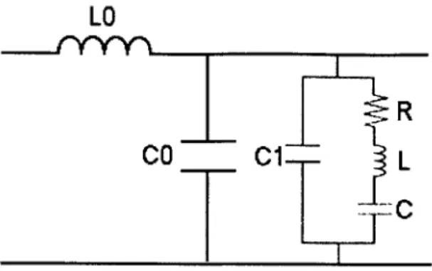
2-10 BVD model of a resonant structure. . . . . 45

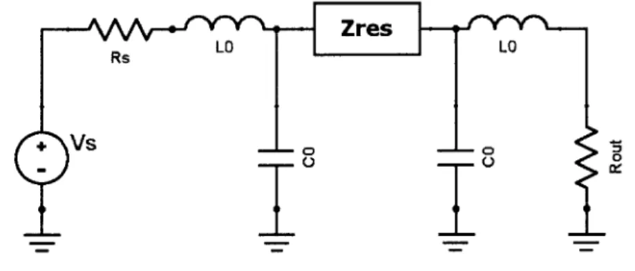
2-11 Equivalent circuit model of the piezoelectric resonator in series with the transm ission line. . . . . 46

2-12 Impedance of the piezoelectric resonator. . . . . 47

2-13 The signal passed through the piezoelectric resonator. . . . . 47

3-1 Unit cell of general lumped element line. . . . . 52

3-2 Simulated value for the phase shift across a transmission line using numerical and full-wave simulations. . . . . 54

(12)

3-4 Equivalent circuit of a Draper resonator placed across a transmission

lin e. _{. . . .}

3-5 Dispersion relation of parallel architecture material. . . . . 3-6 Equivalent circuit of a Draper resonator placed in series with a

trans-m ission line. . . . .

3-7 _{Dispersion relation of series architecture material. . . . .}

3-8 Measured and Simulated S-parameters. .. . . . 3-9 Percent transmitted and phase shift per meter of the designed

meta-m aterial. . . .. . . .

3-10 Length and efficiency comparison of three structures. . . . .

4-1 _{Example of c versus i space, with behavior and uses labeled for each}

quadrant. . . . ..

4-2 Real part of impedance in 6 _{versus p space .. . . . .}

4-3 Extracted measured and simulated material parameters via several dif-ferent m ethods. . . . . 4-4 The extracted permittivity and permeability of the resonator... 4-5 Permittivity and permeability with frequency . . . .

4-6 Permittivity and permeability in 3D . . . . 4-7 1t and c for different parallel capacitances. . . . .

4-8 p and 6 for different series capacitances. . . . .

4-9 it _{and c for different lengths. . . . .}

4-10 p and 6 versus frequency for different lengths. . . . .

4-11 p and c for different widths. . . . .

4-12 p and e versus frequency for different widths . . . . .

4-13 p and e versus frequency for many different resonator sizes.

4-14 Impedance of MEMS metamaterial. . . . . 4-15

4-16

Selecting the length of the resonator by specifying the resonant frequency. Selecting the width of the resonator by specifying the desired im-pedance and material parameters. . . . .

57 58 59 60 63 64 66 70 71 72 78 . . . . 78 . . . . 79 . . . . 81 . . . . 82 . . . . 83 . . . . 84 . . . . 85 . . . . 86 . . . . 87 . . . . 87 88 89

(13)

A-I Conformal mapping of a Coplanar Waveguide to a parallel-plate waveguide. 98 A-2 A force diagram for a cantilever. . . . 100

(14)

THIS PAGE INTENTIONALLY LEFT BLANK

(15)

List of Tables

2.1 Constraints used for paddle resonator optimization . . . . 36

2.2 Optimum dimensions of paddle resonators for three target frequencies. 36

(16)

(17)

Chapter 1 Introduction

The term "metamaterial" refers to any material that is artificially constructed for the purpose of achieving desired properties. In electromagnetics, a metamaterial can be created by constructing a periodic structure with elements of size less than the wavelength of the incoming electromagnetic wave. Because the bulk properties of this material no longer depend on the materials used, but depend on the geometry of the structure, the resulting material can be engineered for any purpose, and can even achieve behaviors that are not found in nature.

The material values of particular interest to the electromagnetics community are the values of permittivity, c, and permeability, p. These values are a characterization of the ability of electric and magnetic fields, respectively, to polarize the medium.

Taken together, e and p determine the speed of electromagnetic propagation through

a medium, as well as many other important values. Through the use of metamaterials, we can create materials with chosen values for 6 _{and p, giving designers great control}

over the many material parameters that depend on those values.

While metamaterials may offer many exciting opportunities in electromagnetics, they also have several drawbacks. Depending on the type of metamaterial, there are problems with large physical size, significant loss, difficult system integration, and low bandwidth. Micro-Electro-Mechanical Systems (MEMS) devices boast small size and easy integration into current circuit fabrication techniques and may therefore provide a solution to some of these problems. In this thesis, I explore the use of

(18)

MEMS resonators to create a metamaterial. Also, I explore some potential uses for

this metamaterial.

1.1 Overview of Chapters

The remainder of this chapter serves as an overview of the relevant work in the field of electromagnetic met amaterials. Additionally, existing met amaterial applications

are discussed. An introduction to MEMS technology follows.

Chapter 2 performs an analysis of two types of MEMS resonator: the paddle and the piezoelectric resonators. Models of each resonator are built and optimized according to specific criteria. The integrity of a signal that is passed through each resonator is determined and compared. The preferred resonator is determined through these criteria, and will become the basic component for the metamaterials designed throughout the remainder of the thesis.

The following chapter, Chapter 3, is dedicated to the evaluation of the disper-sion behavior of a MEMS metamaterial. First, a circuit model is constructed that recreates the behavior of the resonator. Using this model, a method for determin-ing the dispersion relation through an arbitrary structure containdetermin-ing the resonator is constructed. Various structures are simulated and their results are compared. The simulation results are also compared to data obtained from a fabricated structure. Finally, one application for the use of the MEMS metamaterial as a phase shifting element is considered.

After the dispersion analysis, Chapter 4 explores the bulk material parameters that are potentially achievable through the use of a MEMS metamaterial. To de-termine these parameters, a model of the material must be created, and a method for extracting the material values is selected and refined. In order to determine the range of potential material parameters that can be achieved, the dimensions of the resonators used in the model are varied and the results are considered. A method is then introduced by which a designer can create a material with a chosen permittivity and permeability at a specific frequency. Finally, several applications of this new

(19)

material and the new design process are considered.

The final chapter is the conclusion. The conclusion reviews what was accomplished in the thesis. Also, the conclusion analyzes the potential of the applications presented and proposes directions for future work.

Following the conclusion is the Appendix. The Appendix contains two mathe-matical operations that were too large to be included in the main body of the thesis, but provided necessary results for my work. Specifically, the Appendix includes the conformal mapping of a microstrip line to a coplanar waveguide and the calculation of the torque acting on an electrostatically-actuated MEMS cantilever.

1.2 Left-Handed Metamaterials

The idea of a material with simultaneously negative values of permittivity, 6, and

permeability, ft _{was initially presented by Veselago in 1968 [38]. When he was}

consid-ering the definitions of the dispersion relation and index of refraction in an isotropic medium, which depend on the product and the quotient of p and 6, Veselago conjec-tured that a simultaneous change of the signs of both c and / in a medium would have no effect on those relations. Furthermore, in a monochromatic wave, the Maxwell equations and the constitutive equations reduce to Equations 1.1 and 1.2.

[kE] H (1.1)

C W

[kH] = EE _(1.2)

C

From Equations 1.1 and 1.2, we see that the wavevector is real. Recall that the wavevector describes the propagation of the wave in a medium. A real wavevector indicates a propagating wave, while an imaginary wavevector indicates attenuation (an evanescent wave). Therefore because the wavevector in Equations 1.1 and 1.2 is real, electromagnetic radiation is able to move through a material with these values. However, because the wavevector in those equations is negative, the material exhibits

(20)

interesting properties. The index of refraction, defined as Ciii will take the negative

root. The phase velocity, defined as is also negative while the group velocity, d

is still positive. This difference in signs is one of the most interesting properties of left-handed materials. Because the group and phase velocities have opposite signs they are antiparallel, indicating that wave fronts move towards a source in this ma-terial creating a "backwards wave". However, because the Poynting vector, which is defined E x H', is still positive, power travels away from the source and causality is maintained.

Due to the negative index of refraction, these materials are often referred to as NIMs (Negative Index of Refraction Materials). However, in this project, I will re-fer to them as "left-handed metamaterials" (LHMs), emphasizing the left-handed relationship between the electric field, the magnetic field, and the wavevector.

Until recently the study of left-handed materials was merely a thought exercise. However, recent advances in manufacturing technologies make it possible to construct metamaterials that can achieve this behavior. The first work in this direction was

by Pendry. He created a medium consisting of thin wires arranged in a periodic

array

[32].

These wires acted as a plasma medium, whereby 6 varies with frequency,

following the relation of Equation 1.3, where wp is the plasma frequency and 'y is a damping term, both of which are material properties. The value of c was observed to and became negative at some frequencies.

e(w) = 1 - W (1.3)

Pendry next achieved a negative p with a periodic array of metallic loops called Split Ring Resonators[31]. In a medium composed of these rings the permeability, P, varied with frequency, and could become negative. In 1999, Smith combined the rod and ring materials to finally produce a material with simultaneously negative C and

p, a left-handed material [35]. The left-handed behavior (specifically, the negative

index of refraction) of this structure was experimentally verified by Shelby, Smith and

'With complex E and H, it should be E cross the complex conjugate of H, but that designation is omitted here for simplicity

(21)

Schultz [34].

The rod and ring material creates a negative index of refraction because the pe-riodic elements are resonant structures. At specific frequencies, the resonators may fall at integral points along an incoming wavelength. The rod and ring element then stores and radiates energy at its own characteristic frequency, modifying the wave-form. In the proper configuration, the energy storage and radiation of each element will interfere to produce the observed left handed effect.

Due to the complex nature of the rod and ring metamaterial, adjustment and further analysis proved difficult. The complicated geometry and behavior required sophisticated modeling techniques and was difficult to adjust for desired parameters.

A more intuitive interpretation of the material was required. Because the rod and ring

element behaved as a simple resonating element, the material was therefore modeled as an array of lumped circuit elements. The split-ring resonator was abstraced to a model as a circuit consisting of resistors, capacitors, and inductors [18]. This enabled the materials to be analyzed as a circuit, which was a familiar problem with simple solutions. Also, this abstraction made it easier to discern how changes in individual elements would change the global behavior of the medium.

The circuit model of the metamaterial, however, does not necessarily produce in-tuitive results for guided wave applications. Also, the modeling of an entire periodic array was redundant. A further abstraction was needed. It was recognized that dif-ferent geometries of transmission line can reproduce the behavior of circuit elements and that wave propagation through a transmission line is an intuitive analog to wave propagation through a material. As a result, metamaterials have recently been ana-lyzed using a transmission line model. Additionally, a left-handed metamaterial was constructed using transmission lines [8].

When creating transmission lines, the permittivity and permeability of the

sub-strate material are important, as they determine the velocity of propagation, v =

(6)-.5 and the impedance, z = J. These two material parameters are also very important in antenna design because it is important to match the impedance of the feed to the antenna to that of its source. Also, a well-matched substrate impedance

(22)

Figure 1-1: 2D rod and split ring resonator metamaterial. Taken from [34]

will couple well to the air, and radiate efficiently. For these reasons, models of meta-material structure parameters are also further abstracted to produce effective values of E and p.

1.2.1 Existing Left-Handed Metamaterials

The rod and split ring medium built first by Smith is constructed from copper patterns on standard printed circuit board material. To make the two dimensional array that was used for verification, these units were arranged in a grid. A picture of this medium is shown in Figure 1-1. A prism-like shape was built with this grid to verify the left-handed behavior. Radiation was directed at the prism such that the wavevector of the incident waves was perpendicular to a face of the prism. After the radiation traveled through the prism and reached the angled interface with air, the nature of the medium would be revealed. By snell's law, ni sin 01 = n2 sin 02. If the medium is

right-handed, the angle that the wavevector of the emerging radiation makes with the normal vector of the face is positive, but, if the medium is left-handed, the angle is negative. The experiment was performed with radiation at a frequency of 10.5 GHz,

and an index of refraction of -2.7 was observed [34].

The metamaterial constructed for the experiment by Shelby et. al. had some limitations due to the frequency range of the elements that they were using. When the index of refraction neared zero, the wavelength in the material became much larger

(23)

than the size of the entire sample, and the left-handed effects were hard to discern.

Also, the frequency meant that the structure had to be very large

[34].

It was for

these reasons, and a desire to expand the possible application areas of metamaterials that Moser et. al. created a microfabricated rod and split-ring structure [29]. This structure operates at frequencies between 1-2.7 THz, extending the frequency range of left-handed metamaterials by three orders of magnitude, and almost into the infrared. One possible application of the split-ring and rod metamaterial is the production of a "perfect lens," which was predicted by Pendry in 2000 [30]. In the near field of a radiating element, perfect information exists in the radiated waves. However, waves from sub-wavelength features attenuate quickly as the distance from the element increases, and are therefore called "evanescent waves." A left-handed material would amplify these evanescent waves, and therefore be able to reconstruct a perfect image of the source. This potential behavior would create sub-wavelength imaging possibilities. However, the possibility of actually achieving such behavior is under much debate. It is argued that the perfect lens relies on a lossless medium, which is impossible in reality [39]. The resolution of this debate is yet to be discovered.

Another implementation of a left-handed medium is the transmission line meta-material. A transmission line metamaterial was created as a method to more easily interpret left-handed behavior. Also, it had significantly lower loss than the split-ring medium [12]. The transmission line metamaterial was made by building a grid of transmission line elements, each of which recreated the resonant behavior of the split-ring resonator. This structure was constructed using standard printed circuit fabrication techniques and was analyzed in two ways. One method of analysis uti-lized the average phase shift of a signal traveling across a unit cell to determine the bulk behavior of the material[8]. The second method for analyzing the metamaterial verified the bulk material behavior through modeling of wavefronts and S-parameters of guided wave structures with the metamaterial placed inside [3]. From these two methods, the transmission line metamaterial was determined to exhibit left-handed behavior from 1-2 GHz[8].

(24)

index is negative. Also, it is easily scalable for different frequencies, and tunable

by inserting different elements into the structure. These metamaterials have already

been used to make several useful advances in microwave circuits, including smaller antennas, steerable antennas, and improved branch-line couplers[26]. This thesis investigates the hypothesis that a MEMS metamaterial can utilize the advantages already achieved through metamaterials, as well as achieving these behaviors at a smaller size.

1.2.2 Antenna Applications

One application area that I will focus on in this thesis is size reduction of antennas. Specifically, I will look at patch antennas. A patch antenna is a radiating element that is constructed of two parallel conductors separated by a dielectric. The lower plate is used as the ground and is usually larger than the upper, signal plate. A directive antenna is created when the fields between the plates escape through the sides of the patch and the resulting radiation interferes. There are several methods with which one can analyze a patch antenna. One useful method is to model the patch as a thin TM-mode cavity with magnetic walls. The modes of this cavity can be determined and the effect of radiation and other losses are introduced via impedance boundary condition at the walls [5]. The fields radiated by an antenna comes from the modes of the resonator that propagate beyond the resonator.

One important parameter that is used to characterize antennas is the quality factor, Q, which can be defined as [6]:

2w times the mean electric energy stored beyond the input terminals

the power dissipated in radiation

A high value of

Q

can be interpreted as the inverse of the portion of the frequency

band through which the antenna radiates effectively. Therefore a low

Q

is preferable,

as it indicates that the antenna has a broad band, because the impedance varies slowly with frequency.

(25)

102 o 10-Dipole Goubau Efficiency 5% 10% 50% 00% 100 0.2 0.4 0.6 0!8 1 1.2 1.4 kr

Figure 1-2: Plot of the Chu limit for various efficiencies and antennas.

As the size of an antenna is reduced if we continue to think of the structure as a resonant cavity, we see that fewer resonant modes exist. Therefore, fewer propagating modes exist for a smaller antenna and less power can be radiated. From this argument,

when an antenna is made to be smaller, the Q of this antenna becomes very large.

This intuitive derivation has been proven to be defined by a hard limit, called the Chu Limit:

1 + 2(kr)2

kr<1 1

Q

=(1.5)

(kr)3_{[1 + (kr)}2_] _(kr)3

Equation 1.5 represents the lowest achievable

Q

for any antenna that can fit within

a sphere of radius r. In this equation, k is the wavevector. Figure 1-2 shows the Chu limit for various efficiency antennas. Also, data points from existing antennas are plotted. The light blue data points are standard antennas, while the dark blue are metamaterial antennas. Analysis of this plot reveals the value of efficiency in an antenna as well as the capability for metamaterial antennas to approach the optimal Chu limit. Textured o Dielectric Metamaterial Cormic Dipole Reactive o Impedance 0 Peano Substrate Curve

(26)

a) b) c)

Figure 1-3: a) Textured Dielectric Metamaterial, b)Peano Curve, c)Reactive Im-pedance Substrate.

Metamaterial Antennas

There have been several antenna designs that have utilized metamaterials. Three of these designs are included in Figure 1-2, and indicated by the dark blue circles.

The first antenna design is the textured dielectric metamaterial antenna. In this method, the volume between the two plates of the patch antenna is broken into small cubes. The material to be placed in each cube is determined by an optimization algorithm. The resulting dielectric is therefore composed of small pieces of different dielectrics such that the effective permittivity varies with the position on the

dielec-tric. The data shown in

[23]

and [24] indicate that an impressive improvement in

bandwidth can be accomplished by constructing an antenna in this fashion.

A second antenna that fits under the broad topic of metamaterial antennas is an

antenna produced via space-filling curves. In this design, a dipole antenna is folded in a geometric pattern in order to decrease the physical footprint of the antenna without decreasing the electrical length. However, due to this folding the antenna exhibits self-coupling and multiple resonances. One antenna, based on the Peano curve is included in Figure 1-2. The data for the point in Figure 1-2 was taken from [16]. While this design is not constructed of small unit cells, it uses a novel structure to achieve beneficial results, and therefore, I include it as a metainaterial application.

One further use of metamaterials to improve antenna performance is through the construction of a high-impedance ground plane. Also known as a perfect magnetic

conductor (PMC), a high impedance surface has a reflection coefficient of F =

+1.

Therefore, if a dipole antenna were placed directly on this surface, its image current would be in phase, and the radiation performance on that side of the surface would be

(27)

greatly improved. Several types of high-impedance ground planes have been studied, including the use of space-filling curves [16].

The Reactive Impedance Substrate (RIS) is an application that is similar to the construction of a PMC, but aims to alleviate the coupling that occurs between the antenna and the ground plane in that situation. The RIS is composed of a two-dimensional metal grid pattern on top of a metal-backed, high dielectric material. Data from an antenna constructed in this manner is reported in [28] and included in Figure 1-2.

The benefits of using metamaterials in the design of antennas is clear from these examples. However, the field is still quite new, and there are many other designs to be considered, including the potential of MEMS-based designs.

1.3 MEMS

Micro-Electro-Mechanical Systems (MEMS) refers to "the integration of mechanical elements, sensors, actuators, and electronics on a common silicon substrate through microfabrication technology." [1]. The fabrication techniques for MEMS are compat-ible with those for integrated circuits, enabling the use of these two types of structure on a single chip. The ability to have sensors and actuators, as well as logic elements on a single chip opens exciting possibilities for completely integrated microscopic systems that can sense and control their environment.

For this research, I plan to utilize MEMS resonators to construct a metamaterial. The MEMS resonators exhibit a behavior similar to that of the rod and ring element that was used to create te first left-handed metamaterial. The difference between the

MEMS and the rod and ring resonant structures is that the rod and ring element stores

electromagnetic energy, while the MEMS resonator stores energy mechanically (in a physical vibration). However, by putting electrostatically-actuated MEMS resonators in a periodic array similar to the one used for the rod and ring structure, they may exhibit a similarly beneficial electromagnetic behavior. The MEMS resonators are explored more thoroughly in Chapter 2.

(28)

MEMS resonators are good candidates for the creation of a metamaterial for many

reasons. One powerful reason is a great amount of flexibility in resonant frequency. The dimensions of the resonator, which are easily adjustable, dictate its behavior in a predictable manner. This should make a medium created with the MEMS resonators very versatile. Typical measured resonant frequencies of the MEMS resonators range from 100 MHz to 2 GHz. The small size of the resonator is another benefit. Many of the resonators can be combined in an area smaller than a wavelength, creating the possibility for complex metamaterial behaviors and smaller devices. Finally, the ease of integration with existing circuit fabrication processes and circuit structures will make a MEMS-based metamaterial more practical to include in most applications. With all these potential benefits, a metamaterial constructed with MEMS resonators is a worthy purpose.

(29)

Chapter 2 MEMS Resonators

A Micro-Electro-Mechanical System (MEMS) device that exhibits some sort of

me-chanically resonant behavior is called a MEMS resonator. The most common type of

MEMS resonator is the cantilever, which is simply a bar that is secured at one end

and has a natural frequency of oscillation that is determined by its dimensions and material parameters. The cantilever can be driven electrostatically with a conducting pad that creates a potential between itself and the cantilever, creating a force. MEMS resonators are already an important part of devices including microgyroscopes, mi-crovibrators, microengines, and RF systems [27].

I plan to use MEMS to create a metamaterial because the small size, high

Q,

and

ease of integration with circuit fabrication processes that they offer. In this chapter, we will compare two types of electrostatically-driven MEMS resonators and find the resonator that is most fitting for potential use in a metamaterial. The two types are the paddle resonator and the piezoelectric resonator.

2.1 Paddle Resonator

A paddle resonator consists of a rectangular solid (the paddle) suspended over an

open trench by two thin supporting rods that bisect opposite sides of the paddle. Figure 2-1 is a picture of a paddle resonator. When driven by a potential from a conducting pad underneath one side of the paddle, the structure will vibrate. There

(30)

Figure 2-1: A MEMS paddle resonator with the dimensions labeled. From [9]

are several modes of vibration for the paddle, including shifting up and down, left and right, and twisting in a "see-saw" motion. This last mode is the torsional mode, and it is the one that we will focus on, as it occurs at the highest frequencies. We are analyzing the paddle resonator because it is a popular, well-documented design and its torsional mode operates at frequencies nearing the band in which we are interested.

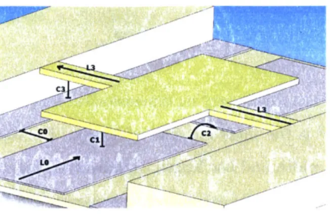
To analyze this resonator, we place it in series with a coplanar transmission line (CPW) such that the middle, signal, line runs below the paddle, exciting the resonance electrostatically. The signal line is broken under the resonator, forcing the signal through the resonator. Figure 2-2 shows this structure. We are then able to model this structure as a circuit, using standard electromagnetic techniques to determine the capacitance and inductance of pieces of the system, based on their geometry and material parameters. This analysis is similar to that performed on other types of metamaterial [18] [8].

The first step in our analysis of the paddle resonator is to analyze the circuit without any resonant behavior. The goal of this step is to determine if the off-resonance behavior of the resonator is desirable for our applications. The next stem in the analysis is to determine how the mechanical resonance changes the behavior of the system. Finally, we determine the performance of the system by calculating the attenuation of a signal that is passed through the resonator.

(31)

Figure 2-2: Three-dimensional model of the paddle resonator with lumped circuit elements labeled.

2.1.1 Broadband Analysis

To analyze the resonator we need to be able to describe its behavior numerically. First, we determine the natural frequency of oscillation and signal attenuation (loss) as a function of geometry. The circuit elements that are produced by the geometry are labeled in Figure 2-2 and the equivalent circuit is shown in Figure 2-3. Using this model, we determine the optimal dimensions of the resonator that will oscillate at a desired frequency with minimum loss.

Natural Frequency

To utilize the resonator, we must be working at and around its natural frequency.

Therefore, in my analysis of these paddle resonators, I needed to be able to deter-mine the natural frequency of a resonator from its dimensions and other material parameters.

The natural frequency of the torsional mode of the paddle resonator is given by Equation 2.1, taken from [9]:

1

= (2.1)

27 I

Where rK is a torsional constant and I is the moment of inertia about the center axis of the paddle along the line of its tethers. The torsional constant can be predicted with the equation from [10]:

(32)

=23

()

ab3 _G _(2.2)

b L

In this equation, / is a slowly varying dimensionless function of the ratio b/a, and

Gaj = 6.7 x 10 10Nm- 2 is the shear modulus of silicon. The dimensions a, b, and L, are the thickness, bar width and bar length, as labeled in Figure 2-1.

The moment of inertia can be calculated by summing the inertia of pieces of the resonator about the same axis. I chose to break the paddle resonator into three pieces: the paddle, and the two tethers. Then I calculated the moment of inertia.

'resonator 'paddle + 2 1tether

S flpaddle( 2 + d2) +₂mtether (a2 ₊_b2)

12 12

= ap (a2 dw + dw + 2a2bL + 2b3 L) (2.3)

12

The mass of each piece was calculated by multiplying the volume of that piece

by p, the density. In silicon, p = 2330 kg m-3. Inserting the value for the inertia

from Equation 2.3 into Equation 2.1, the natural frequency of the torsional mode of a paddle resonator is:

fo _V72 _pa(wd3 _+wd 2_{a + 2a}2_bL₊_2b3_L) (2.4)

In

[9]

the denominator in the equation for the natural frequency only contains

the first term (pawd3). The other terms did not make a difference in their measured

results. Therefore, I also dropped these terms to simplify my calculations, and to adhere to physically realized models.

Analysis of Loss Through Resonator Structure

Creating a circuit from the elements labeled in Figure 2-2, I created the circuit model shown in Figure 2-3. This circuit is the equivalent circuit for a broadband analysis of the paddle resonator. In this context, broadband refers to the off-resonance response.

(33)

Rs LO Vs

F-C2 C1 C1 -0 -of

Figure 2-3: Broadband equivalent circuit model of the paddle resonator

In this condition, the system behaves like the circuit in Figure 2-3 across all frequencies of excitation from V. This broadband analysis was performed to provide a baseline measure of the signal through the paddle.

R8 = Rout = 50Q h

pLh

b ELb C3 =h (2.5)

LO, CO, and C2 are determined by the coplanar waveguide

3.7 of this thesis.

equations from Section

The signal attenuation through this system is determined by comparing the ratio of the voltage across the input resistor, Rs, to the voltage across the output resistor, Rout. These voltages are obtained through straightforward circuit analysis.

When performing the circuit analysis, I assumed the metal was a perfect conductor and ignored losses through fringing fields. Additionally, I ignored the capacitor C2, as its effects are almost purely due to fringing fields, and its size and effects are negligible when compared to the other circuit elements. With these assumptions, the ratio of the output voltage to the input voltage is:

LO

-0 _-o

(34)

Vout __ Rout _(2.6)

Vs Zin

Where Zin is the impedance of the system from the source node. This impedance is calculated using the following equations;

Zin =jwLO- + Z2 (2.7) Z2= jwCO + 1 1 Z3 ( TjwL3 ) + And finally: 1 Z4 = C jwCOF +(jwLO±Rou,)

Substituting the equations for the circuit parameters as a function of physical dimensions (Equations 2.5) into Equation 2.6 and its subsequent definitions of im-pedances, we obtain a mathematical formula for the signal that is passed through the system as a function of the physical size. Additionally, from Equation 2.4, we know the frequency of operation at which we should operate. Therefore, we have an entire mathematical description of the interesting parts of the system (ignoring the physical resonance) as a function of physical dimensions.

Using these equations that describe the electrical behavior as a function of phys-ical size, we can determine the optimal size of a paddle resonator to achieve the desired electrical behavior. In order to find the optimal values for each dimension, I used a random-restart hill climbing algorithm [19], [17]. The algorithm adjusts the dimensions of the resonator model and calculates the loss and natural frequency for that size. From these results, a change is made to the dimensions to step towards an optimum point where the signal loss is at a minimum and the natural frequency is near the desired frequency of operation. When the algorithm converges, it saves the data, and then begins again with random starting values. This is done to increase the

(35)

chances that we will reach a global optimum, instead of becoming trapped at local optima. In this manner, I find the dimensions of a resonator that would function with the least loss near a desired frequency.

Looking at Equations 2.5, some conclusions about the optimal dimensions can be drawn before running any optimization. First, the maximum value for a is desirable because a large a leads to a higher natural frequency (which we need because we want to work in a frequency range that is higher than usually used for these resonators), also the large value of a has no adverse effects to the electrical behavior of the circuit. Another preliminary optimization choice is realized by noticing that a small h will increase C1, and result in less loss. So h should be at the minimum value possible.

However, while it is obvious that increasing d and w will increase C1, and result

in less loss, these changes will also decrease the (already low) natural frequency of the oscillator (via an increased paddle mass and an increased moment of inertia). Similarly, while decreasing b will decrease the loss capacitance C3, it will increase the inductance L3, so without the values of L3 and C3 the overall effect on the system is unclear. These ambiguities are the reason for using the optimization algorithm. The maximum and minimum constraints for each dimension are shown in Table 2.1.

Note that a is fixed at 100pm. This value is the maximum that a can reasonably obtain with conventional fabrication methods. Conversely, although h should be at a minimum, it was included in the optimization because a very small h could cause trouble with the oscillatory motion of the resonator. While we were not considering this motion in the current electrical analysis, it is an important factor to consider and therefore was included to determine if there were any near optimal configurations that did not include the minimum value of h.

An additional constraint in the optimization, denoted by the stars (*) in Table 2.1, is that the values of W and L are related such that 2L + W > 150pm. This constraint is used so the resonator structure is sure to span the transmission line which has a minimum total width of 150pm.

The optimization analysis was carried out for frequencies of 100MHz, 500MHz, and 1GHz. The resulting optima are shown in Table 2.2.

(36)

Table 2.1: Constraints used for paddle

Dimension Minimum Maximum

a 100pm 100pm b mnm 250pm d mnm 250pm h Inm 100Pm L 1pm* 250pm W lpm* 250pm Frequency fo - 10MHz fo + 10MHz

Table 2.2: Optimum dimensions of paddle resonators for three target frequencies.

Target Freq

fo

a b d h L W 7(dB)

100MHz 91.3MHz 100pm 1.31pm 2.56pm inm 27pm 96pm -74

500MHz 491 MHz 100pm 110nm 116nm Inm 27pm 96pm -102

1GHz .995 GHz 100pm 30nm 40 nm mnm 27pm 96pm -131

Judging from the results in Table 2.2, without the mechanical resonance, a paddle structure does not perform well. The best signal strength, at 100MHz, is -74 dB. This means that when 1 Volt is across the input terminals, 0.2 mV can be detected at the output. While this behavior is not terrible, it is also not easy to achieve; obtaining a thickness of 100pm as well as a gap size of Inm would be incredibly expensive, if possible at all. Additionally, when we work in higher frequency ranges, the paddles with dimensions in the tens of nano-meters would be incredibly difficult to fabricate while maintaining the large aspect ratio of 100pm. Because the goal of introducing

MEMS in this thesis is to create an effective, easy, cheap solution, paddle structures

do not appear to fulfill the requirements. The money required could be spent on much more effective systems.

However, in the next section, we add the mechanical resonance to the model of the paddle. This resonance could potentially decrease the impedance enough such that the paddle resonator becomes a viable option for the construction of a metamaterial.

(37)

2.1.2 Resonance analysis

In the previous section, I modeled the gap between the paddle of a paddle resonator and a transmission line that was driving it as a constant-valued capacitor. The

equation that determined the current flowing through the capacitor was IC = C .

If we want to consider the mechanical resonance of the device, this equation no longer

captures the entire behavior of this structure.

To build the more complete model, we must consider how the motion of the paddle changes the electrical characteristics of the system. To do this, we first consider the current passing through the gap from the transmission line to the paddle. The definition of current is the flow of charge. The charge on a capacitor is defined as the voltage across the capacitor times its capacitor. Taking the derivative of this definition of charge to find the complete equation for the current through the capacitor we get:

dQ = dC dV (2.8)

I -V +C .8

dt dt dt

This equation can be thought of as a mechanical device in parallel with an elec-trical one. The currents through the two elements add to produce the total current. The second term of the rightmost portion of Equation 2.8 is the standard electrical definition of current through a capacitor. This represents the electrical component of our parallel system. The other term in Equation 2.8 indicates that the current is also related to the change of capacitance with respect to time. This value changes in our paddle resonator; as the paddle oscillates, the paddle moves closer and further from the driving transmission line, increasing and decreasing the capacitance, and changing the impedance by more than the change in capacitance alone. Therefore, if this component of Equation 2.8 is large, the paddle resonator may pass enough current at resonance to act as desired.

The change in capacitance of the gap between the transmission line and the paddle is related directly to the velocity of the resonator. To find this velocity, we use the standard equation for the harmonic motion of a resonator:

(38)

F F

Figure 2-4: A force diagram for one side of the paddle resonator. (Restoring force is not included)

1±+ IO± +KO -T(Wt, 0) (2.9)

Q

In this equation 0 is the angular displacement of the resonator, as shown in Figure

2.1.2. Its first and second derivatives are indicated by 0 and 0. The variables I and

, are the moment of inertia and torsional constant, respectively. Equations for these

parameters were defined in Equations 2.3 and 2.2 earlier in this chapter. The natural (angular) frequency, wo, can be obtained easily from the natural frequency obtained

from Equation 2.4. The quality factor of the resonator,

Q,

is a product of material

properties and resonator construction. The parameter g is the distance between the

cantilever and the transmission line when 0 is zero. Finally, T indicates the driving

torque on the resonator from the transmission line. Note that this is a function of the voltage on the transmission line (which is a function of wt as well as the angular

displacement, 0).

Before continuing, one note must be made; the rest of the analysis in this section focuses on only one half of the paddle resonator. The other half is assumed to be directly connected to the output and does not contribute to the resonant or electri-cal behavior. This simplification is justified because the goal of this analysis is to determine if the mechanical resonance is large enough to produce any measurable difference in the impedance of our system. In the analysis of one side of the paddle resonator, the resonant behavior is similar to that of the double-sided paddle and the

(39)

electrical behavior is much improved. The resonant behavior is similar because the resonator obeys the same resonance equation, with just a changed moment of iner-tia. The electrical behavior is much improved because the capacitance between the resonator and the driving and sensing transmission lines was the source of the most loss in the previous section. By bypassing the second half of the paddle resonator, we are removing half of that loss. Therefore, the resulting analysis using only one half of the paddle resonator is a viable option to determine if the mechanical resonance of this type of resonator produces enough change in the impedance to make the device a candidate for the use in a metamaterial. With that stated, we continue our analysis

by finding the torque on the bar.

To find an expression for the torque, one first calculates the torque due to one small piece of the bar as a function of theta and its length along the bar. Then the force is summed for all the pieces along the bar to get the total torque. This process is shown in Appendix A.2. The torque that is obtained from the analysis is:

V 2EoW COS 0 L sin _ - 9

T - In (2.10)

2 sinV2

o (g - Lsin g - LsinO

To simplify the analysis we can take the Taylor expansion of T to obtain:

1 w60V2L2 1 wE0V 2L3 1 w60V 2L2 3L2 1 ) 2

T - + - 0+ 2 + (2.11)

4 g 3 g 8 g2 ₍

2

Where the ... indicate the higher order terms that we can ignore. Note that for the Taylor expansion to be valid, the ratio A > sin0. Because this ratio of the_g length of the paddle to the gap is much greater than one for all time in our optimal configurations (shown in Table 2.2), this requirement is always satisfied, and it is therefore safe to use the Taylor expansion result in the following analysis.

Note that the torque is proportional to the square of the electrostatic driving voltage. If we define our input voltage as a DC bias and an AC signal driving voltage:

(40)

Then the torque is proportional to the square of this voltage and has second-order harmonics:

T OC V2 = V2 + 2VcVac sin w + (Vac sin w)2 = v + 2VdcVa7 _{sin w}₊_V2

- cos2w

d2~c \ 22 ac(- 2

Vi ₂" + 2VcVa sin w - ₂ac cos 2w (2.12)

The second order harmonic brought about by the sin W2 term is undesirable. This

value can be neglected if Vc

>

V, which linearizes Equation 2.12. We now can

sub-stitute the equation for torque into the equation of motion of the resonator (Equation

2.9) and solve for 0, the velocity of the cantilever. The velocity of the cantilever can then be used to determine the velocity of the change in capacitance, which in turn will be used to determine the current flowing through our system.

Another important feature of Equation 2.11 is that it includes a term that is independent of the angle 0. This indicates a constant torque that acts on the bar

1. _{This torque is important in our analysis because it creates a constant angle of}

displacement, Odc, that we must consider to ensure that the total angle of displacement

of the bar is not so large that the bar ever contacts the driving line.

To solve for 0 we calculate the transfer function for the resonant behavior of the bar. We get the transfer from Equations 2.9 and 2.11. In this equation s = 1W:

Iw0 1 wE0V2L2 1w,0V 2L3

Is20+ s+ =- 21 - 0+--. (2.13)

Q

4 g2 3 g3

For the frequency-independent component of the displacment angle, Odc, the

trans-fer function consists of all the frequency independent parts of Equation 2.13 (the parts without an s). Also, we only consider the constant torque and the

frequency-independent terms of the voltage. Solving for Odc, we obtain:

'This constant torque is from the force of gravity on the one-sided paddle. In the case of the two-sided paddle, this term is caused by asymmetries in the sides of the paddle[4].

(41)

dc=(VC+ 2wv6oL2

4Kg2

Using the optimal values for a resonator at 100MHz as shown in Table 2.2, we

obtain 0

dc =1.174- 10-6 degrees.

To calculate the frequency-dependent portion of the angular displacement, 0_ac,

we consider the all terms of Equation 2.13. However, when substituting in for V2

from Equation 2.12, we utilize the frequency-independent term of V in the

angle-independent portion of T and the frequency-dependent term in the rest. This is

because, in this frequency analysis, the the constant portion of the torque cannot be

dependent on frequency. After solving for 0

ac, we obtain:

wEoL 2 _(2VcVac) _(2.14)

wcod3 2

-4 2 _gQ182 + S + K - 2

g

The velocity of the bar is 0 = sO. Now, to find the change in capacitance that

will cause the current that we are interested in, calculate the change in capacitance due to the change in 0 of a small piece of the bar of length dl and integrate along the length of the bar.

dC = L COwlCos0 _dl

(2.15)

dO J (g - lsino)2

As mentioned earlier, the current due to the mechanical resonance can be thought of as an independent device in parallel with the electrical device that we analyzed in Section 2.1.1. The impedance of this device is defined as the voltage across it divided as the current through it. Looking at Equation 2.8, we see that the mechanical impedance is therefore:

V 1

'mech

(42)

x 10

7-

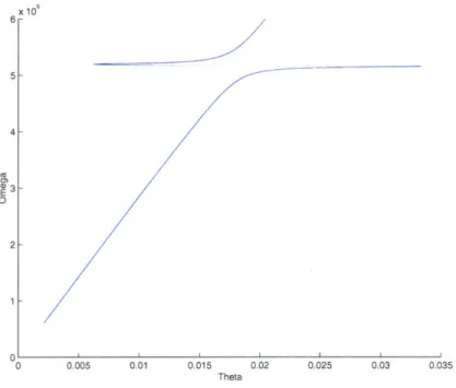
6-Frequency (Hz) 2 25 x10

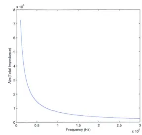
Figure 2-5: Impedance of the paddle resonator. Values are from Table 2.2 and

Q

=

5000.

If we combine this impedance in parallel with the impedance of the electrical component of the system from Equation 2.7, we find the impedance of the entire system. The results from this combination are shown in Figures 2-5 and 2-6. Note in these graphs, the dimensions used are those discovered to be optimum for the 100MHz resonator in Table 2.2 and

Q

= 5000. Figure 2-6 is an enlarged view of the resonant

portion of 2-5.

2.1.3 Evaluation

Using the impedance of the system that includes the mechanical resonant behavior obtained in the previous section, we are able to perform the loss analysis from Section 2.1.1 again, but this time including the mechanical behavior with the hopes that it will cause a large change in the signal that is passed through the system. We use

Equation 2.6, but in this case Ze is the parallel combination of the electrical and

mechanical impedances that was shown in Figures 2-5 and 2-6.

The resulting ratio of output to input voltages

(in

dB) is shown in Figures 2-7

and 2-8. Figure 2-8 is an enlarged view of the resonant portion of 2-7.

These graphs show that, while the mechanical resonance does change the mag-nitude of the signal that is passed through the system, the change is not enough to

(43)

8-

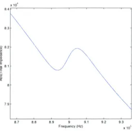
7.9-8.7 8.8 8.9 9 9.1 9.2 9.3

Frequency (Hz) x 10

Figure 2-6: Closer view of resonance of impedance of the paddle resonator.

-55 -60- -65--70 -75- -80--85 -90 1 0 0.5 1 1.5 2 2.5 3 Frequency (Hz)

Figure 2-7: Signal through the paddle resonator. (dB)

8.7 88 8.9 9 9.1

Frequency (Hz)

Figure 2-8: Closer view of resonance of signal passed through paddle resonator.

x 10 8.4 8.3 8.2 2 8.1 x 10 -9.9 -70 -70.1 -70.2 -70,3 -705 --70.5--70.6 -70.7 . 9.2 9.3 x 10'

(44)

bring the signal into any usable region.

Next we will evaluate the Draper piezoelectric resonator in the same manner, to compare its performance to that of the paddle resonator.

2.2 Draper Resonator

The piezoelectric MEMS resonator developed by the Charles Stark Draper Laboratory boasts the characteristics that are desired in a resonator to be used in a metamaterial. It has a simple coplanar design, operates in the desired frequency region, and has a very small footprint. The resonator consists of a piezoelectric substrate (Aluminum Nitride) sandwiched between two electrodes, suspended above a well to allow for vibration. An electric potential across the electrodes of the resonator will induce a mechanical strain in the piezoelectric AlN. An AC voltage can be chosen to match the mechanical resonance of the device. At this frequency the MEMS device exhibits large amplitude vibration and passes current with low impedance.

The piezoelectric equations of state relate the electric field and charge polarization to the mechanical parameters of the resonator. Analysis of these equations can pro-duce a relationship between the voltage across the resonator to the current through it [21]. The existence of this relation indicates that the MEMS resonator can be represented as a collection of circuit elements, as was the split-ring-resonator.

2.2.1 Fabrication and Measurement

The resonator consists of a piezoelectric substrate sandwiched between two conducting bars. In the measured device, the metal bars were constructed of 300 A of Chromium over 1500 A of Platinum. The bar was 4 um wide by 41 um long. The device was fabricated by James Hsiao at the Charles Stark Draper Laboratory. Figure 2-9 shows the S21 parameters that were obtained from measurements of this device.

Design and analysis of MEMS-based metamaterials

Design and Analysis of MEMS-Based

Metamaterials

Jonathan S. Varsanik

©

Design and Analysis of MEMS-Based Metamaterials

by

Jonathan S. Varsanik

Abstract

Q,

Acknowledgments

Contents

List of Figures

[34]

[9]

List of Tables

Chapter 1

Introduction

1.1

Overview of Chapters

1.2

Left-Handed Metamaterials

[32].

1.2.1

Existing Left-Handed Metamaterials

[34].

1.2.2

Antenna Applications

Q

Q

Q

Q

[23]

+1.

1.3

MEMS

Chapter 2

MEMS Resonators

Q,

2.1

Paddle Resonator

2.1.1

Broadband Analysis

()

[9]

pLh

fo

2.1.2

Resonance analysis

Q

Q,

>

Q

Q

Q

2.1.3

Evaluation

(in

2.2

Draper Resonator

2.2.1

Fabrication and Measurement