HAL Id: hal-03015714
https://hal.archives-ouvertes.fr/hal-03015714
Submitted on 20 Nov 2020
HAL is a multi-disciplinary open access
archive for the deposit and dissemination of
sci-entific research documents, whether they are
pub-lished or not. The documents may come from
teaching and research institutions in France or
abroad, or from public or private research centers.
L’archive ouverte pluridisciplinaire HAL, est
destinée au dépôt et à la diffusion de documents
scientifiques de niveau recherche, publiés ou non,
émanant des établissements d’enseignement et de
recherche français ou étrangers, des laboratoires
publics ou privés.
Integration of Theorem-proving and Constraint
Programming for Software Verification
Hélène Collavizza, Mike Gordon
To cite this version:
Hélène Collavizza, Mike Gordon. Integration of Theorem-proving and Constraint Programming for
Software Verification. [Research Report] Laboratoire I3S. 2009. �hal-03015714�
Programming for Software Verification
H´el`ene Collavizza1 and Mike Gordon2
1 Universit´e de Nice–Sophia-Antipolis – I3S/CNRS, 930, route des Colles
B.P. 145 06903 Sophia-Antipolis, France. [email protected]
2 University of Cambridge Computer Laboratory William Gates Building, 15 JJ
Thomson Avenue Cambridge CB3 0FD, UK [email protected] Abstract. A novel approach to program verification combining con-straint programming methods with theorem proving is proposed. Starting from an initial symbolic state and precondition, a program is symbolically executed along all feasible paths and then a post-condition is proved or refuted on the final states. Symbolic execution is by mecha-nised reduction of a formal semantics applied to the program. The con-straint solver incrementally prunes execution paths by testing if condi-tions are feasible in the current state. At the end of each path, deductive theorem proving and constraint solving are tried in sequence. If the theo-rem prover fails, the constraint solver provides a decision procedure for a finite subset of integers. It can also efficiently compute counter-examples. There is a flexible trade-off between speed and assurance. Oracles may be employed as solvers to boost efficiency, but slower formal tools (au-tomatic or interactive) can be used when higher assurance is needed, or the proof requires manual guidance. Theorems proved with oracles are tagged, so the weakest link in a verification is apparent.
The approach has been successfully applied to textbook algorithms and first results show that it is quite efficient. On simple examples most of the proofs are done by the theorem prover, the constraint solver is mainly used to compute counter-examples and check non-linear expressions.
1
Introduction
Our aim is to link together two different and complementary approaches to program verification: (i) constraint solving applied to symbolic execution paths (bounded model checking) and (ii) theorem proving applied to formal semantic specifications (proof of functional correctness).
There is a spectrum of degrees of formality. At one end everything is coded without any mechanical link to formal specifications (e.g. in Java). The formal semantics is just documentation and the only link between it and the verifier code is in the mind of the programmer. At the other extreme everything is me-chanically deduced from a formalisation of the programming language semantics. In the middle – this is the approach described in this paper – lies a mixture of trusted code and theorem proving. Our aim is to explore efficiency/assurance trade-offs obtained by using formal theorem proving tools within a larger verifi-cation framework.
The rest of the paper is structured as follows: first a simple example is used to illustrate key ideas. Next we explain our heuristics for combining constraint solv-ing with theorem provsolv-ing. We then discuss how theorems derived from a formal semantics are used to generate symbolic execution paths. Finally, experimental results are given (including comparisons with previous work).
2
Example: AbsMinus
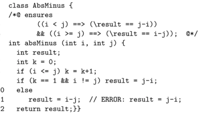
Consider the Java class AbsMinus in Figure 1. This computes the absolute value of the subtraction of inputs i and j. Lines 2-4 give its specification in JML (Java Modelling Language [14]), where ensuresis the postcondition and\result
rep-resents the value returned by the program. The JML specification of AbsMinus is first parsed into a Hoare triple. The translation is not formal, so it is necessary to trust that it faithfully extracts the Java semantics.
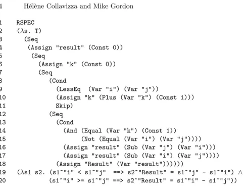
The representation resulting from the initial parsing phase contains three parts: a precondition, a program and a postcondition, which are arguments to a predicateRSPECthat specifies the meaning of the Hoare triple (see Figure 2):
` ∀p c r.RSPECp c r = ∀s1s2. p s1 ∧ EVALc s1s2 ⇒ r s1 s2
EVAL c s1 s2 (see Section 4.1) is true if executing c in an initial state s1
re-sults in a final state s2. The JML precondition is parsed to a predicate on the
initial state, represented by a λ-expression. Since there is no explicit precon-dition in AbsMinus, the parser returns the always-true predicate (λ. T). The program is represented using conventional abstract syntax constructors: Seq is the sequential execution of instructions,Cond is the conditional andSkip is the null instruction. The meaning of these constructors are specified in the defini-tion of EVAL. The postcondition is a relation between the initial and final states, represented as “λs1 s2. · · · ”. Such VDM-style relational postconditions reduce the need for ghost (auxiliary) variables and can neatly represent JML’s \old construct. States are finite maps from strings to values. Values may be scalars (currently just integers) or arrays (finite maps from indexing numbers to values). Details concerning arrays are omitted from this paper. We will write finite maps in the form [x1 7→ v1; . . . ; xn 7→ vn] and the result of looking up a variable x
in a map m as m^x (the actual notations used in the theorem prover are more cumbersome as they explicitly indicate whether values are scalars or arrays). The symbolic execution of AbsMinus proceeds as follows:
A. Compute an initial symbolic state:
["i" 7→ i; "j" 7→ j; "k" 7→ k; "Result" 7→ Result; "result" 7→ result] In this initial state, i, j, k, Result and result are integer variables, represent-ing the symbolic value in the state of the strrepresent-ings (correspondrepresent-ing to program variables) with the same name. Result is the value returned by the program and represents both \result of the JML specification and the expression returned by the Java program.
B. Evaluate the precondition on this initial state: T.
1 class AbsMinus { 2 /*@ ensures
3 ((i < j) ==> (\result == j-i))
4 && ((i >= j) ==> (\result == i-j)); @*/ 5 int absMinus (int i, int j) {
6 int result;
7 int k = 0;
8 if (i <= j) k = k+1;
9 if (k == 1 && i != j) result = j-i;
10 else
11 result = i-j; // ERROR: result = j-i;
12 return result;}}
Fig. 1. AbsMinus program in Java
D. Symbolically execute a path in the program
(a) The first instruction (line 4 in Figure 2) is(Assign "result" (Const 0))). The new state is computed directly from a small-step semantics that has been formally verified (by interactive proof) to correspond to the big-step reference semantics (see part 4.1). The new state is:
["i" 7→ i; "j" 7→ j; "k" 7→ k; "Result" 7→ Result; "result" 7→ 0] (b) The next instruction (line 6) is executed in the same way to get state:
["i" 7→ i; "j" 7→ j; "k" 7→ 0; "Result" 7→ Result; "result" 7→ 0]
(c) The conditional instruction (line 8) is executed using a heuristic that combines the theorem prover (HOL4) and constraint solver to test if the path is feasible (see part 3.2). The condition is first evaluated on the current state, using the semantics of Boolean operations defined for the language (see part 4.1). The result is: i <= j. We then test if this condition is possible according to the precondition (which isT) and the current path (which is also T). First the constraint solver is called to
solve the constraint system: i[-128..127] <= j[-128..127]. It trivially
finds solution (i,-128) (j,-128) (note that the integer format has been fixed to 8 bits here using the heuristic described in 3.2). So condition
i <= j is added into the current path and execution continues on the ‘then’ part of the conditional instruction (line 10).
(d) (Assign "k" (Plus (Var "k") (Const 1)))(line 10) is executed to get: ["i" 7→ i; "j" 7→ j; "k" 7→ 1; "Result" 7→ Result; "result" 7→ 0] (e) The next instruction (line 13) is a conditional branching on:
(And (Equal (Var "k") (Const 1)) (Not (Equal (Var "i") (Var "j")))).
This is is evaluated on the current state to¬(i = j)using the semantics of Boolean expressions. The constraint solver is called to test if this con-dition is possible on the current path. The constraint system is:
i[-128..127] <= j[-128..127] not(i[-128..127] = j[-128..127])
which has a trivial solution. So i=j is added into the current path and execution continues on the ‘then’ part (line 16).
(f) The two last instructions on the path (line 16 and line 18) are executed and the end of the path “i<=j ∧ ¬(i=j)” is reached with symbolic state: ["i" 7→ i; "j" 7→ j; "k" 7→ 1; "Result" 7→ j−i; "result" 7→ j−i].
1 RSPEC
2 (λs. T)
3 (Seq
4 (Assign "result" (Const 0))
5 (Seq
6 (Assign "k" (Const 0))
7 (Seq
8 (Cond
9 (LessEq (Var "i") (Var "j"))
10 (Assign "k" (Plus (Var "k") (Const 1)))
11 Skip)
12 (Seq
13 (Cond
14 (And (Equal (Var "k") (Const 1))
15 (Not (Equal (Var "i") (Var "j")))) 16 (Assign "result" (Sub (Var "j") (Var "i"))) 17 (Assign "result" (Sub (Var "i") (Var "j")))) 18 (Assign "Result" (Var "result"))))))
19 (λs1 s2. (s1^"i" < s1^"j" ==> s2^"Result" = s1^"j" - s1^"i") ∧ 20 (s1^"i" >= s1^"j" ==> s2^"Result" = s1^"i" - s1^"j"))
Fig. 2. Relational specification of AbsMinus program
E. Now we compute the postcondition relation between the initial and final states by β-reducing the application of the λ-expression (lines 19-20) to the symbolic initial and final state, resulting in:3i >= j ==> (j - i = i - j).
We then show that the precondition and the path imply the postcondition:
(i<=j ∧ ¬(i=j)) ==> ( i >= j ==> (j - i = i - j)).
This is easily proved using simplification in the theorem prover (see part 3.3). F. The next step is to backtrack to the previous conditional instruction to ex-plore another path in the program. Execution goes to step D.(e) and tests if the negation of the condition is possible. Since it is possible, execution continues on the ‘else’ part which gives a correct path.
G. The next backtrack goes to step D.(c). Condition ¬(i <= j) is possible so symbolic execution continues on the Skip instruction (line 11), which does not modify the current state. Then the conditional on line 13 is reached. Since the value of "k"in the current state is0, the condition:
(And (Equal (Var "k") (Const 1)) (Not (Equal (Var "i") (Var "j"))))
is evaluated to false and so only the ‘else’ part is explored. This again gives a correct path.
The symbolic execution returns a conditional term that represents the paths that have been successively explored. Each possible value of this term is an outcome which gives the final value of the state. This outcome is preceded by
RESULTwhen the path is correct, and byERRORwhen the path contains an error or 3
Note that the first part of the conjunction in the lambda expression has been eval-uated to true because Result = j-i
if i <= j then (if ¬(i = j) then
RESULT["i"7→i; "j"7→j; "k"7→1; "Result"7→j−i; "result"7→j−i] else
RESULT["i"7→i; "j"7→j; "k"7→1; "Result"7→i−j; "result"7→i−j]) else
RESULT["i"7→i; "j"7→j; "k"7→0; "Result"7→i−j; "result"7→i−j] Fig. 3. Result of symbolic execution of AbsMinus if i <= j then
(if ¬(i = j) then
RESULT["i"7→i; "j"7→j; "k"7→1; "Result"7→j−i; "result"7→j−i] else
RESULT["i"7→i; "j"7→j; "k"7→1; "Result"7→j−i; "result"7→j−i]) else
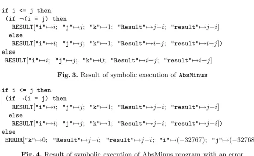
ERROR["k"7→0; "Result"7→j−i; "result"7→j−i; "i"7→(−32767); "j"7→(−32768)] Fig. 4. Result of symbolic execution of AbsMinus program with an error TIMEOUTif symbolic execution failed to reach the end of the program for the given number of steps (see 4.2). Figure 3 shows the result of the symbolic execution of AbsMinus program.
AbsMinus program with an error
We now consider another version of AbsMinus where a ‘copy-paste’ error results in j-ibeing returned instead ofi-j (see line 11 in Figure 1).
When taking pathi>j (line 8, Figure 1) in the program, the symbolic execu-tion ends with final state:
["i" 7→ i; "j" 7→ j; "k" 7→ 1; "Result" 7→ j−i; "result" 7→ j−i]
The relational postcondition is then evaluated toi >= j ==> (j - i = i - j)but the theorem prover fails to show thati > j ==> (i >= j ==> (j - i = i - j))so the constraint solver is called and it trivially finds a first solution(i,-32767)and (j,-32768). This provides a counterexample to the correctness of the program. Figure 4 shows the result of the symbolic execution of AbsMinus with this error.
3
Integrating theorem prover and constraint solver
Before presenting the algorithm of symbolic execution in more detail, we first explain how our theorem prover and constraint solver can be integrated. The goal is to get benefit of both: the theorem prover is good for proving theorems on (infinite precision) integers, but is not able to provide values that satisfies an existentially quantified formula.4 On the other hand, constraint solvers can
efficiently find witnesses for existential quantifications over finite domains and can be slow when the system has no solution, since a complete search through the data domain could be performed.
4
We first briefly explain constraint programming, then describe some tools implemented in our theorem prover (HOL4) and finally describe our heuristics to combine constraint solving and theorem prover to test the feasibility or cor-rectness of program execution paths.
3.1 Constraint programming
Principles Constraint programming is a method for solving hard search prob-lems. Applications include complex scheduling, sequencing, timetabling, routing and dispatching [9]. Constraint programming solvers are based on a branch and prune algorithm that combines local consistencies and efficient search heuristics.
A Constraint Satisfaction Problem (CSP) is defined as: – a set of variables X = {x1, ..., xn},
– a finite set Di of possible values for each variable xi, called domain,
– a set of constraints C = {c1, ..., cn} where ci expresses a relation between
some variables
A solution of a CSP is an assignment of a value from its domain to every variable that satisfies all the constraints.
Arc–consistency [16, 3] is the local consistency used for pruning CSP with finite domains. Let Xj denotes the set of variables that occur in constraint cj.
Constraint cj is arc-consistent if for any variable xi in Xj, each value in domain
Dihas a support in the domains of all other variables of Xj.
We illustrate arc–consistency based branch and prune to solve the CSP: C = {c1 : x1+ x2 < 2, c2 : x21+ x22 ≤ 4, D1 = {0, 1, 2, 3}, D2 = {0, 1, 2, 3}}.
The pruning step starts by checking if constraint c1 is arc–consistent. If value
0 is assigned to x1 then value 1 for x2 satisfies constraint c1 (i.e. value 1 in D2
is a support for value 0 in D0). In the same way, value 1 has support 0 in D2.
But values 2 and 3 have no support in D2 so c1 is not arc–consistent and the
filtering step removes values 2 and 3 from domain D1. For the same reasons,
values 2 and 3 are removed from D2. Then arc–consistency of constraint c2 is
checked. It is arc–consistent for the new domain. Thus, after the filtering step, the domain is: D1= {0, 1}, D2= {0, 1}. Then the search step is enabled. Value
0 is first selected for variable x1and solutions (0, 0), (0, 1) are found. Then value
1 is selected for variable x1 to get the last solution (1, 0).
Calling the solver from the HOL4 theorem prover. Theorem proving tools are implemented as functions written in Standard ML (“ML” for “meta-language”). The HOL4 system provides many predefined functions for proving theorems (e.g. various decision procedures, first-order resolution solvers, com-mands for user-guided interactive proof search). We have augmented these by defining an ML functionextSolvto invoke an external constraint solver. Invoking
“extSolv tm to f” returns a tagged theorem, where the tag (which is propagated
whenever the theorem is used) indicates how the theorem was proved. The first argument, tm, is an existentially quantified term whose satisfiability is to be checked, the second argument,to, is a timeout used to stop the search and the third argument,f, is the integer format used to set the domains of variables in the constraint system. The tagged theorem is built as follows:
– If the constraint solver does not find any solution, then the theorem`(tm=F)
tagged with the string CSPSolver:f is returned. This means that external constraint solver has shown that there exists no value in [−2f −1, 2f −1− 1]
that satisfiestmand thus that¬tm is true for integers coded onfbits. – If the constraint solver finds a solution, then this solution is used to
instan-tiate the existentially quantified variables intmand the theorem `(tm=T)is proved. This theorem is not tagged as externally generated since its proof has been done inside HOL4 using the witness from the solver.
3.2 Heuristics for testing feasibility of paths
A key point of symbolic execution, compared to bounded model checking meth-ods, is that only semantically feasible paths are explored. But this is an improve-ment only if feasibility testing is very fast. Our heuristic for testing feasibility first uses the faster external solver and then, if necessary, slower theorem proving facilities provided by the HOL4 system are tried.
Let Φ be the formula to test, where Φ = ∃i. pre(i) ∧ path(i) ∧ test(i) and i represents input data, pre is the precondition, path is the current path (i.e con-junction of decisions that have been previously taken) and test is the Boolean expression test occurring in a conditional branch. The following two-stage heuris-tic method is used to decide feasibility of Φ.
1. Evaluate test on the current state by symbolically executing the semantics Boolean expressions of the language (see 4.1). If it is true or false then return the corresponding value and stop.
2. Call the constraint solver with a small timeout and a small integer format. (a) If there is a solution, then return true.
(b) It there is no solution, or a timeout, use HOL4’s simplification and integer decision procedures to try to decide the satisfiability of Φ.
Symbolic evaluation (1) is quite efficient and is usually successful when the cur-rent state implies the condition. The constraint solver (2) is also efficient because the domains are small and a timeout is used. Furthermore, if the path is possi-ble for a value inside [−2f −1, 2f −1− 1] it is a fortiori true for a larger domain. The timeout is useful when the path is not possible. In this case, the constraint solver could be very slow to show that there is no solution, since a complete search could be necessary. In this case theorem proving can be faster.
3.3 Heuristic for testing correctness of paths
While efficiency is the key point when testing feasibility of paths, soundness is a priority when testing their correctness. So the theorem prover is called first and only if that fails the constraint solver is called using a large timeout and large integer format. If the solver succeeds then a tagged theorem is returned. If the timeout is reached, or if higher assurance than that provided by the solver is required, then interactive proof can be done.
(∀s. EVAL Skip s s)
∧ (∀s v e. EVAL (Assign v e) s (s+(v,(neval e s)))) ∧ (∀s v. EVAL (Dispose v) s (s-v)) ∧ (∀c1 c2 s1 s2 s3. EVAL c1 s1 s2 ∧ EVAL c2 s2 s3 ⇒ EVAL (Seq c1 c2) s1 s3) ∧ (∀c1 c2 s1 s2 b. EVAL c1 s1 s2 ∧ beval b s1 ⇒ EVAL (Cond b c1 c2) s1 s2) ∧ (∀c1 c2 s1 s2 b. EVAL c2 s1 s2 ∧ ¬(beval b s1) ⇒ EVAL (Cond b c1 c2) s1 s2)
∧ (∀c s b. ¬beval b s ⇒ EVAL (While b c) s s) ∧ (∀c s1 s2 s3 b.
EVAL c s1 s2 ∧ EVAL (While b c) s2 s3 ∧ beval b s1 ⇒ EVAL (While b c) s1 s3)
∧ (∀c s1 s2 v. EVAL c s1 s2
⇒ EVAL (Local v c) s1 (if v ∈ s1 then s2+(v,(s1^v)) else s2-v)) ∧ (∀s p. p s ⇒ EVAL (Assert p) s s)
Fig. 5. Big-step semantics
4
Symbolic execution
We represent programs and specifications as terms in higher order logic and use derived rules and tactics from the HOL4 system to perform parts of the computation, but other parts are programmed directly in ML and Java.
In earlier work (see [8]), semantics preserving transformations, e.g. converting pre and postconditions to a form suitable to submitting to a constraint solver, were performed by unverified Java programs. We have replaced many of these with formal rewriting or custom derived rules5. The implementations of such
truth preserving term manipulations is straightforward, so is not elaborated here.
4.1 Operational semantics
We use mechanised proof to compute symbolic single steps when executing a path (see Point D in Section 2). The formal representation of programs shown in Figure 2 has a standard big-step operational semantics [5] shown in Figure 5. The relationEVAL is the least relation satisfying the conjunction of rules shown in the semantics. A term EVAL c s1 s2 means that executing command c in an initial state s1terminates in a state s2(a more standard notation is hc, s1i ⇓ s2);
neval e s is the value of integer expression e in state s; beval b s is the value of Boolean expression b in s; s+(v,n) is the state obtained from s by making variable v have value n; s^v is the value of v in s, v ∈ s means v is defined in s and s-v is the result of removing v from s.
5 Example: converting formulas of the form ¬((A
1 ⇒ B1) ∧ · · · ∧ (An⇒ Bn) ∧ t) to
(A1∧ ¬B1) ∨ · · · ∨ (An∧ ¬Bn) ∨ ¬t), or converting \forall JML statements to finite
(STEP1 ([], s) = ([], ERROR s))
∧ (STEP1 (Skip :: l, s) = (l, RESULT s))
∧ (STEP1 (Assign v e :: l, s) = (l, RESULT(s+(v,(neval e s))))) ∧ (STEP1 (Dispose v :: l, s) = (l, RESULT(s-v)))
∧ (STEP1 (Seq c1 c2 :: l, s) = (c1 :: c2 :: l, RESULT(s))) ∧ (STEP1 (Cond b c1 c2 :: l, s) =
if beval b s then (c1 :: l, RESULT s) else (c2 :: l, RESULT s)) ∧ (STEP1 (While b c :: l, s) =
if beval b s then (c :: While b c :: l, RESULT s) else (l, RESULT s))
∧ (STEP1 (Local v c :: l, s) =
if v ∈ s then (c :: Assign v (Const(s^v)) :: l, RESULT s) else (c :: Dispose v :: l, RESULT s))
∧ (STEP1 (Assert p :: l, s) = if p s then (l, RESULT s) else (l, ERROR s)) Fig. 6. Small-step semantics
The big-step semantics is not efficient to execute directly,6 so we defined a small-step semantic function STEP1(see Figure 6) and interactively proved that this corresponds to EVAL[17]. Define a small-step transition relation by:
SMALL EVAL (l1,s1) (l2,s2) = (STEP1 (l1,s1) = (l2,RESULT s2))
where l1 and l2 are lists of commands ([] is the empty list and [c] is the singleton list containingc). A routine mechanical proof then establishes:
` ∀c s1 s2. EVAL c s1 s2 = TC SMALL EVAL ([c],s1) ([],s2)
whereTC SMALL EVALis the transitive closure of SMALL EVAL
The functionSTEP1 is efficiently executed inside HOL4 using a call-by-value reduction engine due to Barras [2]. IfSTEP1(l1,s1) = (l2,r)then executing one step of the command at the head of l1in states1results in(l2,r), wherel2are the remaining commands to be executed and r is the result, which can either be RESULT(s2) if the step succeeds or ERROR(s2)if there is an assertion failure. There is a third kind of result,TIMEOUT(s2), which is not generated bySTEP1but
can arise when executing sequence of steps (see below).
4.2 Symbolic execution algorithm
Symbolic execution is by depth first search of feasible paths. A user-specified pa-rameter count bounds the number of steps. (e.g. when programs contain loops). Let pre, path, s1, s2, post be terms as follows:
– pre: precondition (predicate on states represented as a λ-expression) – path: current path (conjunction of decisions taken so far)
– s1: initial state before program execution
– s2: current state after execution of the current path
– post: postcondition (predicate on pairs of states represented as a λ-expression) 6
There are methods of executing inductive relations using techniques adapted from Prolog interpreters, but our theorem prover does not support these.
The initial state s1is automatically built from the program, with logical
vari-ables representing the symbolic values of the program varivari-ables. Let l be the list of terms that represent the instructions of the program (initially this will be[c], wherecis the program being symbolically executed). Let valP re be the precondition evaluated on s1, and valP ost be the postcondition evaluated on
the pair (s1, s2). We assume that we have two functions:
– testPath tests if condition b is feasible on the current path i.e if valP re ∧ path ∧ b has a solution,
– verifyPath tests the correctness of the path i.e if valP re ∧ path ∧ ¬valP ost has no solution7. This function returns the outcome (RESULT s)if the pro-gram is correct along the path and otherwise returns the outcome(ERROR serr) where serr contains the error that has been found.
These two functions call the constraint solver and the theorem prover according to the heuristics described in part 3.2 and 3.3.
The symbolic execution algorithm is detailed in Figure 7. If the last instruc-tion has been reached (point 1) then the correctness of the path is tested. If the maximum number of steps (count) reaches zero (point 3) then an outcome
TIMEOUT(s) is generated. If the first instruction is not a conditional (point 5), then next state is computed and execution continues on the next instruction. If the first instruction is a conditional instruction (point 6) then the feasibility of the condition and the feasibility of the negation of the condition are tested. Note that backtracking is performed when the instruction is a conditional instruction or aWhile-instruction because the two possible paths are explored (i.e points 6 and 13 are both executed).
5
Experimental results
In this section, we report experimental results for a set of textbook algorithms. All experiments were performed on an Intel(R) Pentium(R) M processor 1.86GHz with 1.5G of memory. The theorem prover used is HOL4 and the constraint solver is constraint-programming tool Ilog JSOLVER. Parser from Java to internal syn-tax is built on Eclipse JDT (Java Development Tool).
We first introduce the whole set of examples, then illustrate the main points of our approach and finally discuss related work.
5.1 Set of programs
Tritype Our first example is not a textbook algorithm, however we selected it because it illustrates programs that do not contain loops but have complex conditional statements. This kind of control structure is frequently found in command and control systems. Tritype is a standard benchmark in test case generation since it contains numerous non-feasible paths. This program takes three positive integers as inputs (the triangle sides) and returns a value that determine the type of the triangle (the Java program is given in Appendix 1). This example illustrates how unfeasible paths are cut.
7
this means that valP re ∧ path ∧ ¬valP ost is false for each input value and so that valP re ∧ path ⇒ valP ost is true
execSymb(pre, path, l, s1, s2, count, post) =
1. If l=[] the end of a path is reached so result is verifyPath(pre, path, s1, s2, post)
2. else
3. if count = 0 then the program can’t be executed with the given number of execution steps, so the result is (TIMEOUT s2).
4. else let l = [c,l’]
5. if c is not a control instruction (Cond or While) then call STEP1 to compute the next state s0according to the small-step semantics, then recursively call execSymb(pre, path, l0, s1, s0, count−1, post)
to continue symbolic execution.
6. else let b be the condition of c, then call testPath(pre, s1, path, b)
to know if the condition is possible on the current path
7. if b is possible, take the corresponding path in the program. 8. If c is the conditional (Cond b cthen celse) then
recursively call execSymb(pre, (path ∧ b), [cthen, l0], s1, s2, count, post)
to execute the then part.
9. If c is the loop instruction (While b cwhile) then recursively call
execSymb(pre, (path ∧ b), [(While b cwhile), l0], s1, s2, count, post)
to enter the loop.
10. if b is not possible, take the corresponding path in the program. 11. If c is the conditional (Cond b cthen celse) then
recursively call execSymb(pre, (path ∧ ¬c), [celse, l0], s1, s2, count, post)
to execute the else part.
12. If c is the loop instruction (While b cwhile) then recursively call
execSymb(pre, (path ∧ ¬b), l0, s1, s2, count, post)
to exit the loop.
13. Call testPath(pre, s1, path, ¬b) to know if the
negation of the condition is possible on the current path and take the corresponding path as explained above.
Fig. 7. Symbolic execution algorithm
Sum of the n first integers computes the sum of the n first integers. The specification is that it returns n × (n + 1)/2 (where n is the data input). This illustrates how loops are handled and how symbolic execution sets a constant value to n and thus avoids getting a non-linear term at the end of the path. Sum of integers from P to N computes the sum of the integers from p to n where p and n are input data (see Appendix 2). The precondition is that p is less or equal to n and the postcondition is that the value returned is n × (n + 1)/2 − (p − 1) × p/2. This example illustrates how the constraint solver is called when the term to be verified at the end of the path is non-linear.
Binary search is the well known binary search program that determines if a value x is present in a sorted array a. We also consider an incorrect version of this program where a copy-paste error has been inserted (see Appendix 3). Bubble sort with precondition is a bubble sort algorithm where a precondi-tion sets the values of the array to be sorted in decreasing order and to contain the values from a.length − 1 to 0. This example is from Mantovani et al. [1].
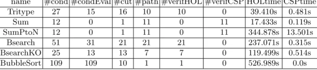
name #cond #condEval #cut #path #verifHOL #verifCSP HOLtime CSPtime Tritype 27 15 16 10 10 0 39.410s 0.481s Sum 12 0 1 11 0 11 17.433s 0.119s SumPtoN 12 0 1 11 0 11 344.878s 13.501s Bsearch 51 31 21 21 21 0 237.071s 0.315s BsearchKO 25 13 13 7 7 0 119.499s 0.514s BubbleSort 109 109 10 1 1 0 526.989s 0.0s
Table 1. Experimental results
5.2 Discussion
Table 1 shows statistics on the solving process for our set of examples. In this table, #cond (resp. #condEval and #cut) is the number of conditions reached in the program (resp. that have been decided using simplification in HOL4 and that have been proven false). #path is the number of feasible paths. #verifHOL (resp. #verifCSP) is the number of paths that that have been verified using HOL4 (resp. using the constraint solver). HOLtime (resp. CSPtime) is the time spent by HOL4 for proofs and symbolic execution (resp. with the CSP solver). For Sum and SumPtoN, we verified all numbers of loop steps from 0 to 10, and for Bsearch and BubbleSort program, the length of the array has been set to 10. Tritype As shown in table 1, half of the conditions were decided by evaluating the condition on the current state. This is due to the fact that many tests in the Tritype program (see Appendix 1) are on a local variable which is assigned constant values, according to the number of triangle sides which are equal. Sum of the n first integers This example illustrates how loops are handled. Our symbolic execution algorithm is bounded by the maximum number of in-structions that can be executed, which provides a bound for loop unwinding. All paths through the loop containing less than this maximum number are explored. For theSumexample, adding loop entrance and exit conditions (see points 9 and 12 in figure 7) sets a constant value to variable n. For example, when the loop has been entered 5 times, the term to be verified is:
∃n.(n ≥ 0) ∧ (0 ≤ n ∧ 1 ≤ n ∧ 2 ≤ n ∧ 3 ≤ n ∧ 4 ≤ n ∧ ¬(5 ≤ n)) ∧ ¬(10 = n ∗ (n + 1)/2). Since n must satisfy both 4 ≤ n and ¬(5 ≤ n) it follows that n = 4, so the postcondition ¬(10 = n ∗ (n + 1)/2) trivially holds.
The results in Table 1 show that 11 paths have been explored (entering 0, 1, 2, ..., 10 times into the loop) and that all the paths were solved with the constraint solver. This is because simplification in HOL4 doesn’t handle non linear terms. However, since the value of n is constant as explained above, the constraint solver efficiently verifies this term.
Sum of integers from p to n If we now start the sum with input data p, the decisions taken to enter the loop, or not, won’t set the value of n, since it will depend on p. For example, the term below is the term to be verified when the loop has been entered 5 times:
∃np.(n ≥ 0 ∧ p ≥ 0 ∧ p ≤ n) ∧ (p ≤ n ∧ p + 1 ≤ n ∧ p + 2 ≤ n ∧ p + 3 ≤ n ∧ p + 4 ∧ ¬(p + 5 ≤ n)) ∧ ¬(p + (p + 1) + (p + 2) + (p + 3) + (p + 4) = n ∗ (n + 1)/2 − (p − 1) ∗ p/2)
The conditions on the path imply that n = p + 4, but this does not set any constant value for n. The results in Table 1 show that execution time for HOL4 is 20 times slower than time for the Sum program. This is due to the fact that simplification rules take more time trying to simplify the term before they finally fail. Also, the constraint solver takes 100 more times than for theSum program because here, the term to be verified is not instantiated.
Binary search Table 1 shows that all paths were solved with the theorem-prover and that more time was spent with the constraint solver for theBsearch
with an error since it was called to find the errors.
Two errors were found in the incorrectBsearchprogram (Appendix 3). The first for path ¬(a4=x)∧x<a4∧¬(a1=x)∧¬(x<a1) for data input x =-32768and
a =[-32768,-32768,-32768,-32767,-32766,-32766,-32766,-32766,-32766,-32766]. Value x is first searched on the left part of the array, so index lef t = 0 and right=3. Then it is searched on the right part, but the error in the program set the right index instead of the left one and so lef t = 0 and right=0. Since the array is initially sorted, a0 ≤ a1 and the condition ¬(x < a1) in the path implies that a0 ≤ x.
Thus the value is then searched on the right. Again the error in the program modifies the right index to get lef t = 0 and right = −1. So the execution stops with result = −1 while value-32768is in the array.
Note that this example also illustrates our heuristic for testing paths: the theorem-prover has been called for testing two paths because a time-out was reached with the constraint solver.
Bubble sort Table 1 shows that we explored the unique feasible path in this program and that all conditions were decided by evaluating the condition on the current state. In fact, the precondition set the initial values of the array. The 10 conditions that were false correspond to the 10 times where condition j < a.length − i − 1 was false (i.e. exiting the inner loop).
5.3 Discussion of related work
We first discuss previous work based on constraint programming for software val-idation. Then we contrast our symbolic execution algorithm to bounded-model checking (BMC). And last we discuss other approaches that merge theorem proving and automatic formal verification methods.
Constraint logic programming was first used for test generation of programs [12, 13, 15]. Gotlieb et al. [4] showed how to represent imperative programs as constraint logic programs and used predicate abstraction and conditional con-straints within a constraint logic programming framework. This test-generation methodology was generalised and applied to bounded program verification in [7], where a hybrid constraint system including Booleans for control and integers for data was generated and solved. In order to avoid exploring spurious execution paths, the approach presented in [8] introduces the symbolic execution algorithm used here which prunes unfeasible paths using constraint-based solvers8.
8 More precisely, this previous approach combined the ILOG CPLEX MIP Mixed
Inte-ger Programming tool which is based on the simplex algorithm with ILOG JSOLVER we used in this paper
This symbolic execution algorithm is similar to bounded-model checking ap-proaches in the sense that it explores paths of bounded length (see [10] for a recent survey). But it differs in at least two ways. First, the feasibility of paths is tested with efficient solvers and thus only feasible paths are explored. Second, each path is verified separately and thus the formulas to be proven are smaller. This is better adapted to theorem proving or constraint solving methods, which are not tailored to handle large formula with a complex Boolean structure.
The alternative BMC method for software consists in building a formula whose models correspond to program execution paths of bounded length that violate a property. The satisfiability of this formula is checked by replacing arith-metic operators by bit-vectors operators to obtain a propositional formula which is solved using efficient SAT solvers. CBMC [6] is one of the most popular tools that implements BMC for checking C programs. In recent work [1], Armando et al. used SMT solvers to verify linear programs with arrays.
A comparison of performances between BMC and our previous approach that combines symbolic execution and constraint programming is provided in [8]. Performances of the approach presented in this paper are in average two hundred times slower. But most of the proofs are done within the theorem prover.
Another interesting piece of work that combines theorem proving with au-tomatic solvers is presented in [11]. The Why/Krakatoa/Caduceus platform is based on the Why language, which is dedicated to program verification. Both Java and C programs are translated to Why programs. A tool based on a Weak-est Precondition calculus generates verification conditions for interactive provers, such as Coq or Isabelle and automatic provers such as Simplify or SMT solvers Yces. This approach differs from ours because it doesn’t combine dynamic theo-rem proving with other automatic solvers. On the contrary, it generates a set of verification conditions, a subset of which can be checked by a theorem prover. Experiments with the Why platform, showed that our approach is less efficient on the tritype program (8.85s with Why and 39.8s for our approach), but that our approach was applicable to the binary search program while Why approach was not (unless an invariant is provided).
6
Future work
We mentioned in the introduction that the work reported here lies in the mid-dle of a verification tool implementation spectrum with unverified tools at one end and everything computed by deduction inside a theorem prover at the other end. In the future we plan to explore other points in this spectrum. In particular we would like to perform the complete symbolic execution and path extraction within a theorem prover and compare performance and scalability with the ap-proach described here. Preliminary experiments suggest that this is feasible, but there are efficiency challenges. However, in applications requiring certification, having high assurance that verification is sound is valuable, so it is useful to cal-ibrate the cost of increasing soundness assurance, even if for some applications the price is too high.
Acknowledgements
We would like to thank Michel Leconte for much help and advice with JSOLVER. Many thanks also to Andreas Podelski for fruitful discussions on bounded model checking and for suggesting one of the examples.
References
1. Armando A., Mantovani J., and Platania L. Bounded Model Checking of C Pro-grams using a SMT solver instead of a SAT solver. Proc. SPIN’06. LNCS 3925, Pages 146-162.
2. Bruno Barras. Programming and Computing in HOL. Theorem Proving in Higher Order Logics, 13th International Conference, TPHOLs 2000, Portland, Oregon, USA, August 14-18, 2000. LNCS 1869: 17–37.
3. C. Bessiere, E.C. Freuder, and J.-R. Rgin. Using constraint metaknowledge to reduce arc consistency computation. in Artificial Intelligence 107: 125–148, 1999. 4. Botella B., Gotlieb A., Michel C. Symbolic execution of floating-point
computa-tions. Software Testing, Verification and Reliability, 16:2:97–121,2006.
5. Juanito Camilleri and Tom Melham, Reasoning with Inductively
Defined Relations in the HOL Theorem Prover, Technical
Re-port 265, Computer Laboratory, University of Cambridge, 1992.
http://www.comlab.ox.ac.uk/tom.melham/pub/Camilleri-1992-RID.pdf
6. Clarke E., Kroening D., Lerda F. A Tool for Checking ANSI-C programs. Procs of TACAS 2004, LNCS 2988: 168–176, 2004
7. Collavizza H. and Rueher M. Software Verification using Constraint Programming Techniques. Procs of TACAS 2006, LNCS 3920: 182-196, 2006.
8. Collavizza H., Rueher M., and van Hentenryck P. A Constraint-Programming Framework for Bounded Program Verification. Proc. of CP200, LNCS 5202: 327– 341,2008, Springer-Verlag.
9. Rina Dechter: Constraint Processing. Morgan Kaufmann publisher,2003
10. Vijay D’Silva, Daniel Kroening and Georg Weissenbacher. A Survey of Automated Techniques for Formal Software Verification. IEEE Transactions on Computer-Aided Design of Integrated Circuits and Systems, Vol 27, N 7, July 2008. 11. Fillitre J.C., Claude March.The Why/Krakatoa/Caduceus Platform for Deductive
Program Verification Proc. CAV’2007, LNCS 4590: 173-177, 2007.
12. Gotlieb A., Botella B. and Rueher M : Automatic Test Data Generation using Constraint Solving Techniques. Proc. ISSTA 98, ACM SIGSOFT (2), 1998. 13. Daniel Jackson and Mandana Vaziri, Finding Bugs with a Constraint Solver, ACM
SIGSOFT Symposium on Software Testing and Analysis, 14–15, 2000. 14. JML home page http://www.cs.ucf.edu/ leavens/JML/
15. Sy N.T. and Deville Y.: Automatic Test Data Generation for Programs with Integer and Float Variables. Proc of. 16th IEEE ASE01, 2001.
16. A. Mackworth : Consistency in networks of relations. Journal of Artificial Intelli-gence, pages 8(1):99–118, 1977.
17. Tobias Nipkow. Winskel is (almost) Right: Towards a Mechanized Semantics Text-book. In Foundations of Software Technology and Theoretical Computer Science, LNCS 1180, 1996, 180-192.
Appendix 1: Tritype program
/** program for triangle classification
* @return 1 if (i,j,k) are the sides of any triangle * 2 if (i,j,k) are the sides of an isosceles triangle * 3 if (i,j,k) are the sides of an equilateral triangle * 4 if (i,j,k) are not the sides of any triangle */ class Tritype {
/*@ requires (i >= 0 && j >= 0 && k >= 0); @ ensures
@ (((i+j) <= k || (j+k) <= i || (i+k) <= j) ==> (\result == 4))
@ && ((!((i+j) <= k || (j+k) <= i || (i+k) <= j) && (i==j && j==k)) ==> (\result == 3))
@ && ((!((i+j) <= k || (j+k) <= i || (i+k) <= j) && !(i==j && j==k) && (i==j || j==k || i==k)) ==> (\result == 2)) @ && ((!((i+j) <= k || (j+k) <= i || (i+k) <= j) && !(i==j && j==k) && !(i==j || j==k || i==k)) ==> (\result == 1)); @*/
static int tritype (int i, int j, int k) { int trityp = 0; if (i == 0 || j == 0 || k == 0) trityp = 4; else { trityp = 0; if (i == j) trityp = trityp + 1; if (i == k) trityp = trityp + 2; if (j == k) trityp = trityp + 3; if (trityp == 0) { if ((i+j) <= k || ((j+k) <= i || (i+k) <= j)) trityp = 4; else trityp = 1; } else { if (trityp > 3) trityp = 3; else {
if (trityp == 1 && (i+j) > k) { trityp = 2;
} else {
if (trityp == 2 && (i+k) > j) { trityp = 2; } else { if (trityp == 3 && (j+k) > i) { trityp = 2; } else { trityp = 4; } } } } } } return trityp; } }
Appendix 2: Sum of integers from P to N
/* Computes the sum of integers from p to n. */
public class SumFromPtoN{
/*@ requires (n >= 0) && (p >= 0) && (p<=n) ; @ ensures \result == n*(n+1)/2 - (p-1)*p/2; @*/
int sum (int p,int n) { int i = p; int s = 0; while (i<=n) { s = s+i; i = i+1; } return s; } }
Appendix 3: Bsearch program
class Bsearch {
/*@ requires (\forall int i; (i >= 0 && i < a.length -1); a[i] <= a[i+1]); @ ensures
@ ((\result == -1) ==> (\forall int i; (i >= 0 && i < a.length); a[i] != x)) @ && ((\result != -1) ==> (a[\result] == x));
@*/
int binarySearch (int[] a, int x) { int result = -1;
int mid = 0; int left = 0; int right = a.length -1;
while (result == -1 && left <= right) { mid = (left + right) / 2; if (a[mid] == x) result = mid; else { if (a[mid] > x) right = mid - 1; else
left = mid + 1; //ERROR: right = mid - 1; }
}
return result; }
}
Appendix 4: Bubble Sort program
/* Bubble sort with a precondition:
* the array contains numbers between 0 and a.length * sorted in decreasing order
*/
class BubbleSort {
/*@ requires (\forall int i; 0<= i && i < a.length; a[i] == (a.length-1)-i); @ ensures (\forall int i; 0<= i && i < a.length-1; a[i]<=a[i+1]); @*/
static void sort(int[] a) { int i=0;
while (i<a.length-1){ int j=0;
while (j < (a.length-i)-1) { if (a[j]>a[j+1]) {
int aux = a[j]; a[j]= a[j+1]; a[j+1] = aux; } j=j+1; } i=i+1; } } }