Lasso and probabilistic inequalities for multivariate point processes

This paper defines an information flow control model, namely Tuple-Based Access Control (TBAC), inspired by lattice-based and Mandatory Access Control (MAC) models [23] as well as

To our knowledge there are only two non asymptotic results for the Lasso in logistic model : the first one is from Bach [2], who provided bounds for excess risk

To our knowledge there are only two non asymptotic results for the Lasso in logistic model: the first one is from Bach [2], who provided bounds for excess risk

In this paper, we prove a process-level, also known as level-3 large deviation principle for a very general class of simple point processes, i.e.. nonlinear Hawkes process, with a

Davydov’s inequality has the following known application to the control of the variance of partial sums of strongly mixing arrays of real-valued random variables. 0)

In the whole paper (X i ) 16i6n is a sequence of centred random variables. We shall obtain here a value of ρ which depends on conditional moments of the variables. We also want

Using large deviation techniques, it is shown that T c I is equivalent to some concentration inequality for the occupation measure of a µ- reversible ergodic Markov process related

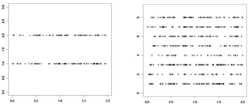
A multivariate Hawkes framework is proposed to model the clustering and autocorrelation of times of cyber attacks in the different group.. In this section we present the model and