HAL Id: hal-01446070
https://hal.archives-ouvertes.fr/hal-01446070v2
Preprint submitted on 28 Jan 2017
HAL is a multi-disciplinary open access archive for the deposit and dissemination of sci-entific research documents, whether they are pub-lished or not. The documents may come from
L’archive ouverte pluridisciplinaire HAL, est destinée au dépôt et à la diffusion de documents scientifiques de niveau recherche, publiés ou non, émanant des établissements d’enseignement et de
A Formalisation of the Generalised Towers of Hanoi
Laurent Théry
To cite this version:
A Formalisation of the
Generalised Towers of Hanoi
Laurent Th´ery
Laurent.Thery@sophia.inria.fr
Abstract
This notes explains how the optimal algorithm for the generalised towers of Hanoi has been formalised in the Coq proof assistant using the SSReflect extension.
1
Introduction
The famous problem of the towers of Hanoi was proposed by the french mathematician ´Edouard Lucas. It is composed of three pegs and some disks of different size. Here is a drawing of the initial configuration for 5 disks1
:
Initially, all the disks are pilled-up in decreasing order of size on the first peg. The goal is to move them all to another peg. There are two rules. First, only one disk can be moved at a time. Second, a larger disk can never be put on top of a smaller one.
The towers of Hanoi one of the classical example that illustrates all the power of recursion. If we know how to solve the problem for n disks, then the problem for n + 1 disks can be solved in 3 steps. Let us suppose we want to transfer all the disks to the last peg. The first step uses recursion and moves the n-top disks to the intermediate peg.
The second step moves the largest disk to its destination
The last step uses recursion and moves the n disks on the intermediate peg to their destination.
This simple recursive algorithm is also optiomal: it produces the minimal numbers of moves. In particular, if we look at each recursion depth, the
key idea is that largest disk always moves once from its current peg to its destination.
The generalised version of the towers of Hanoi considers an arbitrary initial configuration and an arbitrary final configuration. These two configu-rations must be valid : there is no larger disk on top of a smaller disk. The problem is to find an algorithm that generates the minimal nunber of moves that connects the two configurations. Here, the naive recursive algorithm is still applicable to solve the problem but does not lead to an optimal algo-rithm. This can be illustrated by 3 disks when trying to go from the initial configuration:
to the final position
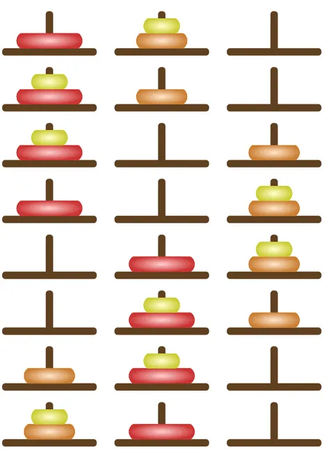
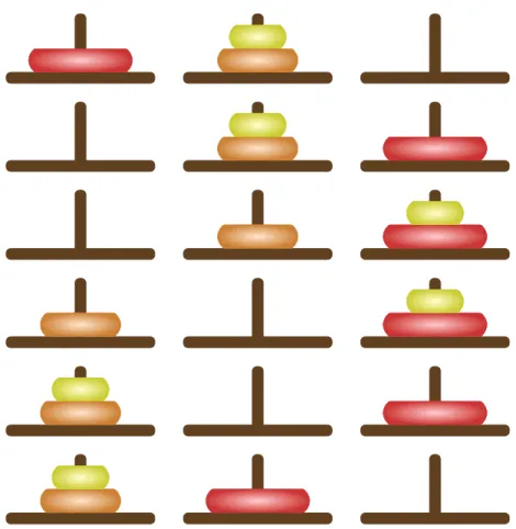
If the naive recursive approach, that tries to move the largest disk only once, leads to a 7-move long solution as depicted in Figure 1 at page 12. The optimal solution requires instead to move the largest disk twice and is 5-move long as depicted in Figure2at page 2. In the following, we explain how the generalised towers of Hanoi has been formalised in the Coq proof assistant and how an algorithm that solves this problem has been proved correct.
2
The formalisation
In this section, we present the different elements our formalisation, start-ing with pegs, disks, configurations and moves, then we describe the naive recursive algorithm and finally the optimal one.
2.1
Pegs
The set of natural numbers strictly smaller than three I3 is used to represent
the three pegs.
Definition peg := I3.
An operation that is frequently used in the algorithm is, having two arbitrary peg p1 and p2 to get the third one, This is done by the function opeg using
some arithmetic:
Definition opeg p1 p2 : peg := inord (3 − (p1+ p2)).
where inord is the function that injects a natural number into the type In.
2.2
Disks
A parameter n is used. A disk is then an element of In.
Definition disk := In.
The comparison of the respective size of two disks is simply performed by comparing their natural number.
2.3
Configurations
Disks are ordered from the largest to the smallest on a peg. This means that a configuration just needs to record which disk is on which peg. It is then defined as a finitite function from disks to pegs.
Definition configuration := {ffun disk → peg}.
Note that in this encoding, we do not have invalid configurations.
A configuration is called perfect if all its disks are on a single peg. It is the case for the initial and final configurations in the standard towers of Hanoi. The constant function that always returns p is then the perfect configuration where all the disks are on the peg p.
Definition perfect p:= [ffun d ⇒ p].
We also need two functions to build configurations. The first one builds a new configuration from a configuration c by putting all the disks of size strictly smaller than m on the peg p: this new configuration is perfect at depth m.
Definition mk perfect m p c := [ffun d ⇒ if d < m then p else c d].
The second function performs a single change on the configuration c : the disk d is moved to the peg p.
Definition setd d p c2 := [ffun d1⇒ if d1= d then p else c d1].
2.4
Moves
A move is defined as a relation between configuration. A parameter m is introduced. It represents a bound on the size of the disk that has been moved. Its purpose is to let us perform proof by induction: the induction is then performed on the depth of the moves m rather than on the number of disks n.
Definition movem : rel configuration :=
[rel c1 c2 | [∃d1 : In, [&& d1< m, c1d1 6= c2d1, [∀d2, d16= d2 ⇒ c1 d2 = c2 d2], [∀d2, c1 d1= c1 d2 ⇒ d1≤ d2] & [∀d2, c2 d1= c2 d2 ⇒ d1≤ d2]]]].
The definition simply states that there is a disk d1 htat fulfills five conditions.
Its size is smaller than m. It is has moved. It is the unique disk that has moved. No disk is in on top of d1 in c1. No disk is on top of d1 in c2.
Trivial facts first need to be derived. For example, the move relation is cumulative and symmetrical.
Lemma moveW m1m2: m1 ≤ m2→ subrel movem1 movem2.
Lemma move sym m c1 c2 : movem c1 c2 = movem c2 c1.
A first interesting is then that before and after a move, all the disks smaller than the disk that has moved are all pilled up on the same peg:
Lemma move perfectl m d c1 c2 :
movemc1c2 → c1 d6= c2 d→ c1 = mk perfect d (opeg (c1 d) (c2 d)) c1.
Lemma move perfectr m d c1c2:
movemc1c2 → c1d6= c2 d→ c2 = mk perfect d (opeg (c1 d) (c2 d)) c2.
An important corollary is that if a disk d moves twice on different pegs then the two configurations after the first move and before the second one are perfect configurations at depth d.
Lemma move twice d c1c2 c3 c4 :
c16= c4 → c1 d6= c2d→ c3d6= c4 d→
moved.+1 c1 c2 → connect moved c2 c3→ moved.+1c3c4→
c2 = mk perfect d (opeg (c1 d) (c2 d)) c2 ∧
c3 = mk perfect d (c1 d) c2.
This is a key lemma that is used to get a direct lower bound (2d
−1) on the number of moves that are needed for connecting c2 are c3. We will explain
this later.
In order to be able to decompose paths under the movem.+1 relation, two
inversion lemmas are needed. The first one checks if the disks m moves. If it is the case, it singles out its first move.
Inductive pathS spec (d : In) c : seq configuration → bool → Type :=
pathS specW : ∀cs, path moved ccs → pathS spec d c cs true |
pathS spec move : ∀c1 cs1 cs2,
path moved c cs1→ c d 6= c1d→ moved.+1 (last c cs1) c1 →
path moved.+1 c1 cs2→ pathS spec d c (cs1++ c1 :: cs2) true |
pathS spec false : ∀cs, pathS spec d c cs false.
The decomposition is presented as an inductive predicate in order to get the decomposition by the direct application case: pathSP tactic on a path. The second inversion lemma considers a path at depth d + 1 for which the disk d may have moved but at the end it remains on the same peg. It builds the ”restricted” path for which the disk does not move.
Lemma pathS restrictE d c cs :
path moved.+1c cs → last c cs d= c d →
{cs1 |
[∧
path moved ccs1,
last c cs1 = last c cs &
size cs1 ≤ size cs ?= iff cs1 = cs ]}.
The number of moves of the restricted path gets strictly smaller only if there is a move of the disk d in the path cs.
2.5
Naive algorithm
Our definition of the naive algorithm works at depth m, starts with a con-figuration c and tries to move all the disks of size less than m to the peg p. The strategy works as follows. If the disk m is already on the peg p, there is nothing to do at depth m: the algorithm is recursively called at depth m −1. Otherwise, the disk m needs to be moved. The algorithm is first called at depth m − 1 to move all the disks of size smaller than m − 1 to the intermediate peg p1. Then, the disk of size m is moved to the peg p and
finally the algorithm is called a second time to move the disk of size smaller than m − 1 to the peg p. Formally, this gives2
:
Fixpoint rpeg path rec m c p:= if m is m1.+ 1 then
if c m= p then rpeg path rec m1c p else
let p1:= opeg (c m) p in
let c1 := setd m p (mk perfect m1p1c) in
rpeg path rec m1 c p1++ c1 :: rpeg path rec m1c1p
else [::]
Definition rpeg path c p:= rpeg path rec n c p.
Note that c1 is configuration after the disk m has been moved to the peg p:
all the disks smaller than m are on the intermediate peg p1.
The first basic property that needs to be proved is that this algorithm is correct: what is build is a path that goes from the configuration c to the perfect configuration on peg p
Lemma rpeg path correct c p(cs := rpeg path c p) : path(move n) c cs ∧ last c cs = perfect p.
This directly gives the fact that any configuration is connected to any perfect configuration
Lemma move connect rpeg c p : connect (move n) c (perfect p).
Since the relation is symmetric, this gives that any two configurations are connected.
Lemma move connect c1 c2 : connect (move n) c1 c2.
There is always a solution to the generalized tower of Hanoi.
If we are only interested by the size of the solution, it is possible to give an algorithm that computes the size of the connection given by the naive algorithm.
Fixpoint size rpeg path rec m c p:= if m is m1.+ 1 then
if c m= p then size rpeg path rec m1 c p else
let p1:= opeg (c m) p in
size rpeg path rec m1 c p1 + 2 m
1 else0.
Note that in this version, there is only one recursive call. The justification for this comes from the fact that this algorithm returns 2m
−1 when called on a perfect configuration c that is different from p.
Lemma size rpeg path rec 2p m p1p2c (c1 := mk perfect m p1 c) :
size rpeg path rec m c1 p2 = (2 m
−1)(p16= p2).
This gives us directly that it computes the actual size of the naive algorithm.
Lemma size rpeg path rec pr m c p:
size(rpeg path rec m c p) = size rpeg path rec m c p.
As a matter of fact 2m
−1 is the maximum a naive solution can get
Lemma size rpeg path rec pr m c p: size rpeg path rec m c p ≤ 2m
−1.
With these results, it is possible to prove the optimality of the naive algorithm for the special case where the initial configuration is perfect.
Lemma rpeg path rec min m c1 pcs (c2:= mk perfect m p c1) :
path (move m) c1cs → last c1 cs = c2 →
size rpeg path rec m c1 p≤ size cs ?= iff(cs = rpeg path rec m c1 p).
Note that we also prove that the optimal solution is unique. The proof works by a double induction: one induction on the depth m and another strong induction on the size of cs. So, when proving the step case at depth m, the property is known to hold for all paths at depth m − 1 and for paths at depth m which size is strictly smaller than cs. We then simply do a discussion on the number of moves the disk m does in the path cs:
- If it does not move, the inductive hypothesis for m − 1 gives directly the result.
- If it moves once, the path cs mimics the strategy of the naive algo-rithm at depth m. So, combining the two applications of the inductive hypothesis for m − 1 (one before and one after the move) gives the result.
- If it moves more than once, there are two possibilities. Either the disk visits a peg more than once (this is always the case if the disk moves
more than two times). In this case, the lemma pathS restrictE gives us a stricly smaller path on which we can apply the inductive hypothesis on the size. Either the disk has moved twice on different pegs. The lemma move twice tells us that if we consider the path the first move and before the second, it connects two perfect configurations at depth m − 1. So the inductive hypothesis for m − 1 and the lemma size rpeg path rec 2p tell us that its size is greater than 2m−1
−1. The same holds for the path after the second move and the final configuration. Altogether, this gives a size for cs (not considering the path before the first move of the disk m) that is larger than 1 + (2m−1
−1) + 1 + (2m−1
−1) = 2m
. This is strictly more than the bound 2m
−1 for the naive algorithm given by the lemma size rpeg path rec pr.
This ends the proof.
2.6
Optimal algorithm
In order to define the optimal algorithm, we first define the symmetric of the naive algorithm that goes from a perfect configuration to any configuration by simply reversing the path.
Definition lpeg path rec m p c := rev (belast c (rpeg path rec m c p)). Definition lpeg path p c:= lpeg path rec n p c.
This algorithm is clearly correct and optimal.
The optimal algorithm is defined recursively in order to find the first disk that has to be moved. When this disk is found, it simply chooses the best solution between moving it directly to where it has to go (going from c1 to
c3 then c2) and moving it twice (going from c1 to c3 then c4 and fimally c2)
using the intermediate peg p. The computation of these two solutions can use the naive algorithm since one of the two configurations that are connected is perfect, so we know it is optimal.
Fixpoint hanoi path rec m c1c2 :=
if m is m1.+1 then
if c1 m= c2 m then hanoi path rec m1c1c2 else
let p:= opeg (c1 m) (c2 m) in
let n1:= size rpeg path rec m1 c1 p+ size rpeg path rec m1 c2p in
let n2:= size rpeg path rec m1 c1 (c2 m) +
2m
1 + size rpeg path rec m1 c2 (c1 m) in if n1≤ n2 then
let c3 := setd m (c2 m) (mk perfect m1 p c1) in
rpeg path rec m1c1 p ++ c3 :: lpeg path rec m1 p c2
else
let c3 := setd m p (mk perfect m1 (c2 m) c1) in
let c4 := setd m (c2 m) (mk perfect m1 (c1 m) c1) in
rpeg path rec m1c1 (c2 m) ++ c3:: rpeg path rec m1 c3 (c1 m)
++ c4:: lpeg path rec m1(c1m) c2
else [::].
Definition hanoi path c1 c2 := hanoi path rec n c1 c2.
It is then easy to derive that this algorithm is correct. The proof for opti-mality is similar to the one for the naive algorithm : we simply show that the largest disk cannot move three times in the optimal solution.
Lemma hanoi path correct c1c2 (cs := hanoi path c1 c2) :
path(move n) c1 cs ∧ last c1cs = c2.
Lemma hanoi rec min m c1c2cs :
path(move m) c1 cs → last c1 cs = c2 →
size(hanoi path rec m c1 c2) ≤ size cs.
3
Conclusion
We have presented a formalisation of the generalised towers of Hanoi. The formalisation clearly benefits from the SSReflect library. In particular, finite function have been a convenient tool to encode configuration. Most of the proofs are elementary. Without surprise, the difficult part is to get the optimality results. We had to device two dedicated inversion principles in or-der to mechanise the case distinctions that were needed. The complete proof is available athttp://www-sop.inria.fr/marelle/Laurent.Thery/Hanoi.