Physics-informed detection and segmentation of type II solar radio bursts

(1)

HAL Id: hal-02923001

https://hal.inria.fr/hal-02923001

Submitted on 26 Aug 2020

HAL is a multi-disciplinary open access

archive for the deposit and dissemination of

sci-entific research documents, whether they are

pub-lished or not. The documents may come from

teaching and research institutions in France or

abroad, or from public or private research centers.

L’archive ouverte pluridisciplinaire HAL, est

destinée au dépôt et à la diffusion de documents

scientifiques de niveau recherche, publiés ou non,

émanant des établissements d’enseignement et de

recherche français ou étrangers, des laboratoires

publics ou privés.

Physics-informed detection and segmentation of type II

solar radio bursts

Joseph Jenkins, Adeline Paiement, Jean Aboudarham, Xavier Bonnin

To cite this version:

Joseph Jenkins, Adeline Paiement, Jean Aboudarham, Xavier Bonnin. Physics-informed detection

and segmentation of type II solar radio bursts. British Machine Vision Virtual Conference, Sep 2020,

Virtual, United Kingdom. �hal-02923001�

(2)

JENKINS ET AL.: PHYSICS-INFORMED SOLAR RADIO BURST LOCALISATION

Physics-informed detection and

segmentation of type II solar radio bursts

Joseph Jenkins1 josephrjenkins@gmail.com Adeline Paiement2 adeline.paiement@univ-tln.fr Jean Aboudarham3 jean.aboudarham@obspm.fr Xavier Bonnin3 xavier.bonnin@obspm.fr

1_{Computer Science Department}

Swansea University Swansea, UK

2_{Université de Toulon, Aix Marseille}

Univ, CNRS, LIS Marseille, France

3_{Observatoire de Paris/PSL}

Paris, France

Abstract

Type II solar radio bursts have proven to be a useful tool for gaining insights into the behaviour of complex solar events and for forecasting and mitigating their damages on Earth. In this work, we detect and segment the occurrence of type II bursts in solar radio spectrograms, thereby facilitating the extraction of parameters needed to gain insight into solar events. We utilise prior knowledge of how type II bursts drift through frequencies over time to assist with these tasks of detection and segmentation. A new adaptive Re-gion of Interest (ROI) is proposed, to constrain the search to reRe-gions that follow the burst curvature at a given frequency. It comes with an implicit data normalisation that reduces the variance of burst appearance in the data, hence simplifying the learning process from small datasets. We demonstrate the effectiveness of our methodology using a simple and popular HOG and logistic regression detector and basic segmentation based on voting and background subtraction. On a custom dataset representative of different levels of solar activity, at a wavelength range where no other detection algorithm currently oper-ates, our adaptive ROI significantly improves over traditional sliding windows. In future work, it may be applied to other, state-of-the-art, machine learning algorithms.

1 Introduction

Solar radio bursts have become an increasingly important topic of study due to their relation with events of space weather that threaten society, including solar flares, Solar Energetic Particle (SEP) events, and Coronal Mass Ejections (CMEs). Type II bursts in particular are often good indicators of CMEs and SEPs. Their physical properties (e.g. frequency range, duration (both total and per frequency channel), intensity, presence of a harmonic (secondary signal approx. parallel to the main one as in Fig.1left), speed of frequency drift (usually called drift rate) which translates as the curvature of the signal when visualised in a spectrogram, see Fig.1) can give important insights into the physics of these events and mechanisms that produced them. Their automated detection also permits the forecasting of terrestrial arrival times of space weather events [6], thereby allowing the initiation of

(3)

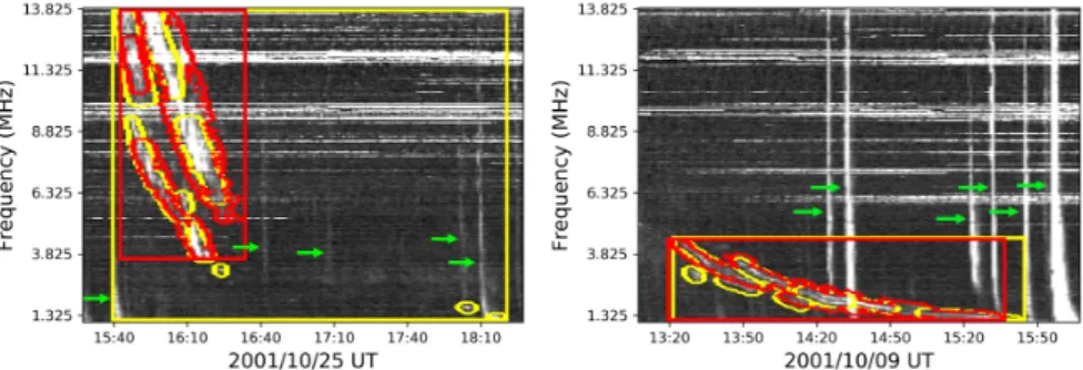
Figure 1: Detection and segmentation (yellow: ground-truth, red: predicted) of type II solar radio bursts, in the presence of type III bursts (green arrows) and background noise (inc. RFI as bright horizontal lines). Note the different shapes/curvatures of the type II bursts at dif-ferent frequency ranges. We show contrast enhanced spectrograms for ease of visualisation.

precautionary measures for damage mitigation. This is because radio bursts reach Earth within ∼8 minutes at light speed, whereas the slower particles of SEPs and CMEs take a few tens of minutes to a few days, respectively. In this work, we are concerned with the detection and segmentation of type II solar radio bursts. Segmentation is a preliminary step towards their future physical characterisation. Type III bursts are more frequent than type IIs, and they present similar features (strong signal against noisy background). They may come individually or in groups, which sometimes overlap with a type II. Thus, we also consider these in our study to help with disambiguation.

Of the various burst types pertinent to space weather, type II bursts are arguably the most difficult to detect. While individual type III bursts have consistent appearances as thin vertical lines (see Fig.1), type II bursts have more complex and varying shapes. Their curvature is a result of their characteristic frequency drift, with a continuously decreasing rate which can be modeled by a function of (the decreasing) frequency [1]:

d f/dt = −α fψ_, ₍₁₎

where α and ψ are a scaling factor and power index on the frequency f , respectively. Type II bursts may appear at different ranges of frequency, and have different parameters, hence a wide range of curvatures are possible. This complicates the learning process for pat-tern recognition techniques and imposes the use of larger training sets. Furthermore, their low rate of occurrence coupled with the requirement of expert knowledge during annotation makes the production of large and representative datasets challenging. To overcome these issues, we propose to integrate knowledge of the drift model into the machine learning based detector to implicitly reduce the variance within the data. In Section3, following (1), we define a curved ROI that adapts its curvature based on the frequency being searched. In do-ing so, we ensure that any detections are constrained to the possible physics. In addition, the curved ROI’s data is normalised across all frequencies, which inherently reduces the shape variation of type II bursts across the dataset. We demonstrate in Section5 that these two effects simplify the learning over our small dataset.

Only few works [3,7,9] have addressed the detection of type II bursts due to their com-plexities, and none have attempted their segmentation or physical characterisation. [9] pre-sented a general detector for radio bursts of types II, III and IV, but only prepre-sented results for

(4)

type III bursts. [7,9] used classical image processing methods (e.g. thresholding, morpho-logical operations), while, in a recent unpublished work, [3] used an off-the-shelf YOLO [8] deep learning detector trained from simulated types II and III bursts. The only method that we know of, that used information on the physics of the type II burst signal, is that of Lobzin et al. [7] who proposed a first exploitation of the drift model to simplify the task of detection. They found that ψ ≈ 1 for their dataset (ψ ∈ [0.6, 1.3]), which allowed the rearrangement of frequencies from f to 1/ f to significantly reduce their curvature. The problem of burst detection thus became greatly simplified to the problem of detecting straight lines, solved with a Hough transform. However, this data transform drastically reduces the resolution for the high frequencies because many of these frequencies are mapped to the same (rounded) 1/ f values. Lobzin et al. [7] resolved that situation by discarding full (now overlapping) rows of the spectrogram. This results in a significant degree of information loss: 33.5% of discarded channels for their dataset that covers the 25–180 MHz frequency range with their instrument conveniently sampling the 75–180 MHz high frequencies at a resolution twice lower than the 25–75 MHz low frequencies, and 56.3% for ours in the 1.075–13.825 MHz range because of uniform sampling of frequencies.

In summary, the main contributions of this work are: 1) a new strategy for integrating knowledge on the physics of a signal into a detector. This integration allows better constrain-ing the detection and segmentation problems, while implicitly reducconstrain-ing the variance in the appearance of the data. We demonstrate that these effects result in a simplification of learn-ing that requires fewer trainlearn-ing samples. The knowledge integration is done through 2) a new curved ROI that is demonstrated within a classical HOG-based sliding window detector, and may be more generally applied within other algorithms. 3) A new dataset of type II and type III radio bursts with detection and type II segmentation annotations. 4) A new method for detecting and segmenting type II radio bursts. It is demonstrated on the 1.075–13.825 MHz range, but its reliance on machine learning would allow re-training it at other frequencies.

In the rest of this article, we introduce our new dataset in Section2, and our curved ROI in Section 3. The detection and segmentation pipeline is presented in Section4, and evaluated in Section5. Concluding remarks and future works are provided in Section6.

2 Type II/III solar radio bursts dataset

We utilise data from the instrument Wind/WAVES [2] and its radio receiver RAD2. The re-ceiver contains 256 frequency channels linearly spaced from 1.075–13.825 MHz, and a tem-poral resolution of 16 sec averaged to 1 min. 244 type II bursts are sampled from NASA’s catalogue of 511 radio-loud (i.e. generating type II bursts) CMEs [5] over 1997–2016 in-clusive. These bursts, when occurring at high frequency, are often preceded by intense type III bursts. In general, type III bursts happen frequently with an intensity and vertical shape that match that of high frequency type II bursts, and may cause confusions for a detector. Therefore, for our negative samples, we consider both the ‘empty’ (but generally noisy) background as well as 242 type III bursts randomly sampled from the HFC catalogue1. The Sun’s level of activity (i.e. the occurrence rate of solar events) follows an 11-year cycle, commonly illustrated by the varying number of sunspots that may be observed at its surface over time. We consider three levels of activity in our experiments (high, low, and medium), with corresponding periods of time defined from the central 40%, outer 20%, and remaining

(5)

Type II Type III Background # windows 244 : 49 / 89 / 106 242 : 47 / 89 / 106 245 : 48 / 88 / 109

Table 1: Class distribution of the dataset’s event windows. A breakdown of the numbers per solar activity level is given as: total : low / med / high.

Duration (mins) Frequency range (MHz) Burst size (px) # sub-bursts # harmonics # lone events 48.30 (40.56) 7.07 (3.66) 929 (687) 4.52 (3.62) 1.72 (0.70) 54 Table 2: Statistics on our 244 type II bursts in ‘mean (std)’ format. Only annotated (i.e. visible) parts of the bursts are considered in calculating the metrics. ‘Lone event’ are bursts with no strong noisy signals (e.g. type III, calibration, RFI) in the close (∼30 pixels) vicinity.

40% of Gaussian distributions fitted on the sunspot numbers of each cycle.

Our dataset contains different levels of annotation. Firstly, 3-hour windows are annotated as containing either ‘Type II’, ‘Type III’, or ‘Background’. The Type II and Type III windows start 15 min prior to their associated burst. Some Type II windows may also contain type III bursts (noisy signals), as they sometimes occur concurrently. On the other hand, since our focus is on detecting type II events, Type III windows are considered as negative samples and we ensure that they do not contain any type II bursts. Furthermore, we ensure that our selection of negative windows (Type III and Background) does not overlap with positive Type II windows to avoid information leaks. The distribution of windows per class and activity level are provided in Table1. Secondly, within the Type II windows, the associated burst has been manually segmented with expert validation. Some statistics over the annotated bursts are presented in Table2. Type III bursts have not been segmented due to their very short duration and known occurrence time. Thirdly, multiple ROIs have been sampled from each 3-hour window to generate a training set for our classifier. For the Type II and Type III windows, the ROIs of corresponding class focused on the known location of the burst. More details on the ROI selection will be provided in the Experiment section.

The signal of type II bursts often appears sporadically as a collection of smaller segments, denoted as sub-bursts. In our dataset, individual sub-bursts are contoured, as seen in Fig.1. Some sub-bursts, such as the lower frequency tails, may be difficult to identify due to either drifting below the frequency covered by a given sensor or dipping below the intensity of the background. This makes it challenging to recover a burst’s full frequency range and duration. However, for the purpose of space weather forecasting, detecting and characterising only the visible parts of the burst is generally satisfactory. Thus, we focus on this task both in the preparation of our dataset and in the design of our detector, without addressing the challenge of detecting the fainter or missing tail sub-bursts.

There is a hierarchy of sub-bursts forming harmonics of a burst event. However, for our purpose of semantic segmentation, considering sub-bursts is enough and we did not group them into harmonics and bursts in our method, although harmonics are annotated in the dataset. Including this hierarchy in the method may be done in future works when retrieving a burst’s parameters (including the number of harmonics).

(6)

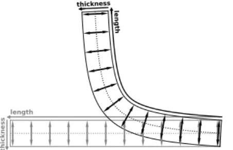
Figure 2: Definition of the adaptive curved ROI based on the drift trajectory curve (1) (black dotted-line), and re-shaping into a normalised version.

3 Adaptive curved ROI

We propose to use the drift rate model presented in (1) to constrain the extraction of ROIs that better match the physics of the signal. A straightforward approach would be to adapt the aspect ratio of the (rectangular) ROI to the range of frequencies that it covers. However, given the curvature of the signal, rectangular ROIs are ill-suited and may enclose a large part of background. In addition, their rescaling to a fixed aspect ratio before analysis by a classifier may not effectively normalise the appearance of bursts.

To overcome these issues, we propose a curved ROI that matches the drift trajectory of the burst. As illustrated in Fig.2, a 2D curved region is constructed from the 1D curve de-fined by (1) by restricting it to a specified frequency range and adding thickness to it. Based on (1), the shape (i.e. curvature) of the ROI will adapt to its starting and end frequencies. Overall, the adaptive curved ROI is defined by 5 parameters: α, ψ, starting frequency, length along the curve, and thickness. By construction, when centred on a type II burst, the ROI contains mostly useful signal without enclosing as much background as a rectangular ROI.

Since the ROI adapts to and follows closely the shape of the type II bursts, it may be used to normalise it, hence greatly reducing the variance caused by the frequency-drift de-pendency. This may be done simply by straightening out the ROI into a rectangular region, as illustrated in Fig.2. This straightening is performed by sampling along regularly spaced normals of the drift trajectory curve, using nearest neighbour interpolation as a proof of concept (although other interpolation methods are usable). The rate of normal sampling is chosen to match the resolution of the data, i.e. 1 pixel of distance along the curve between samplings, hence minimising the information loss from the ROI transformation. This lim-ited information loss is an advantage over the normalisation of [7]. The resulting rectangular window is suitable for classical computer vision algorithms, including learning-based ones. In addition, the reduction of variance from curvature normalisation allows the learning task to be greatly simplified, even for simple machine learning models paired with our limited number of training samples.

4 Type II burst localisation

We demonstrate our adaptive curved ROI using a popular detector and simple segmentation procedure. As illustrated in Fig.3, the localisation pipeline includes preprocessing of the spectrogram to improve contrast and signal to noise ratio (Section4.1), followed by a sliding

(7)

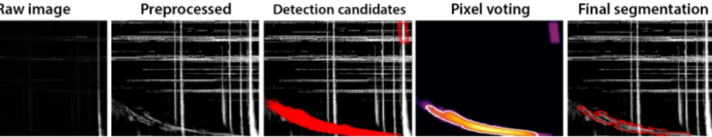
Figure 3: Overview of the type II burst detection pipeline. Col. 4 shows the result of pixel voting (white) overlaid on the log counts of detection candidates (see Section4.3).

window detector that implements our adaptive curved ROI (Section4.2). The candidate detections are finally aggregated into a segmentation using a pixel-wise voting procedure (Section4.3). In our proof-of-concept, we apply our detector to 3-hour windows.

4.1 Preprocessing

As can be seen in Fig.3left, our spectrograms suffer from a very low contrast. However, they also contain some speckle noise, coming from various sources including non-solar (e.g. the galaxy), which hinders the direct application of contrast enhancement techniques. There-fore, we aim to subtract away the speckle background while preserving the type II signal. We approximate it by a Gaussian fitted on a 12-hour window for each frequency channel. We first clip each frequency channel to a minimum of µ + λ σ of its Gaussian distribution (with λ a tunable parameter, optimised to 0.5 in our experiments), thus only keeping the highest values where bursts may be visible. Second, we remove isolated objects with low connectivity i.e. non-clipped areas smaller than a threshold (we found that 5 px works well in our experiments). This step is motivated by the random nature of the speckle noise making it unlikely for large clumps of signal to form, whereas the spatially correlated nature of burst signal makes it much more likely, and hence will be preserved. RFI noise and calibration signals appear as strong horizontal and vertical lines, respectively, with similar distribution to that of the signal of interest. We choose not to target these for noise removal, and instead rely on the classifier’s ability to learn about their typical shapes. After noise removal, any missing samples (from instrument errors) are replaced using a mean filter on 3x5 px win-dows, and we augment the contrast using a sigmoid transform with gain 10, followed by histogram equalisation. The result of preprocessing is illustrated in Fig.3.

4.2 Sliding window detection

The adaptive curved ROI defined in Section3may be used within a sliding window detector just like any traditional rectangular ROI. Indeed, it may be slid across the image, both along the horizontal axis (time) and the vertical one (frequency), with its shape and curvature auto-matically adapting to its frequency (i.e. vertical location). The straightened and normalised (rectangular) region that the ROI defines may be provided as input to a classifier in the same straightforward way as for a classical rectangular ROI.

Regardless of its location in the image, our ROI can be described by three properties: length and thickness as defined in Section3 and Fig.2, and drift trajectory decided by α and ψ (i.e. the curve obtained for our spectrogram’s range of frequencies for given values of its parameters). We find empirically that combinations of 3 different thicknesses, 4 lengths, and 4 drift trajectories (illustrated in Fig.4left), as reported in Table3, provide a reasonable

(8)

Figure 4: Optimised sliding procedure for our adaptive curved ROI: temporal scanning for all 4 choices of drift trajectory (left) followed by ROI straightening (see Fig.2) and scanning along the drift trajectory curve for different ROI lengths and thicknesses (right).

Drift trajectory α 1.47×10−4 6.19×10−5 9.54×10−5 1.21×10−4

ψ 0.25 0.58 0.82 0.5

Length (px) 42 74 132 164

Thickness (px) 12 18 24

-Table 3: Choice of discrete parameters for the ROI.

coverage of the burst shapes in our dataset. This provides 48 anchor ROIs (with adaptive shape based on vertical location) to be slid over the spectrogram.

It is worth noting that, for a given temporal position and drift trajectory, pixels within overlapping sliding regions would undergo the same ROI straightening operation multiple times. Therefore, for efficiency, we apply the straightening procedure to the full-lengthed drift curve (i.e. across all frequencies) rather than to its individual ROIs. Our sliding window algorithm is the following: for each of the 4 choices of drift trajectory (spanning the entire frequency range), we first scan the temporal axis (Fig.4left). Second, using the maximum thickness parameter, each maximum 2D curved region is straightened into a rectangular grid. In this transformed space, the different choices of thickness and length result in rectangular 2D ROIs that may scan the space along the axis corresponding to the 1D curve (i.e. drift trajectory), as illustrated in Fig.4right.

The sliding ROIs are passed to a HOG [4] and logistic regression classifier. Parameters of HOG are listed in Table4. Given the sporadic appearance of type II bursts as a collection of smaller sub-bursts (see Section2 and illustrations in Fig.1), the classifier is trained on various combinations of neighbouring sub-bursts rather than full bursts. This naturally aug-ments the size of the training data. Consequently, the sliding window procedure results in a set of candidate curved detections covering various sub-bursts, as illustrated in Fig.3.

4.3 Post-processing and segmentation

The candidate detections focusing on sub-bursts are ill-suited for a classical non-maximum suppression procedure. However, we may use them as a basis for a semantic segmentation of burst signal. Indeed, their shape is designed to mostly contain burst signal and little background. Thus, we may assume that a pixel that belongs to multiple detections and multiple sub-bursts is likely to be part of the burst. The final segmentation may be refined using knowledge on the background from the preprocessing stage.

We tally up the number of detections for each pixel and retain the pixels with a high (log) total (i.e. pixel voting) using an empirical threshold, as illustrated in Fig.3. An optimal value for this threshold may be difficult to find, since a too high value may exclude large

(9)

Cell size 3 × 3 pixels Block size 4 × 4 cells Block stride 3 × 3 pixels Block overlap (due to stride) 3_/₄

Number of bins 10 Gamma correction No Signed gradients Yes

Padding 12 pixels along the length dimension of the ROI Table 4: Parameter values of our HOG descriptors.

parts of the signal, while a too low threshold would introduce false positives. To overcome this difficulty, we use a two-stage process which first selects the core parts of the burst using a high threshold, followed by a refinement of these parts only using a lower threshold. We finally discard any pixels that overlap with the background known from preprocessing to obtain the final segmentation in Fig.3right.

5 Experiments

Since no previous works attempted to localise type II bursts from the frequency range of our data, we cannot compare against existing burst detection methods. Instead, we first evaluate the advantages of our proposed ROI over the classical rectangular ROI. Second, we present the performance of our type II localisation, including both detection and segmentation, when considering all and individual solar activity levels.

For detection purposes, we consider that any intersection of the segmentation mask with the contoured groundtruth results in a successful detection. This choice may result in the number of false positives to inflate substantially whenever the segmentations are fragmented. Therefore, we group neighbouring pixels (with a proximity of 10 px) into a single event prior to checking for an intersection. Type II bursts being rare events, this grouping is unlikely to merge individual bursts.

Table5presents precision, recall and F-score for detection, as well as global IoU consid-ering all pixels of the testing set, and average IoU per detected event to examine how well individual (successfully detected) events are contoured i.e. how many sub-bursts are found or missed. Results are averaged over 25 folds, and std are omitted due to lack of space. The methods’ parameters are tuned individually for each tested scenario using grid search. They are also tuned separately for evaluating the detection and segmentation performances. Indeed, given our definition of true detection, a stricter (sub-optimal) segmentation, that misses more parts of the bursts, but produces fewer false positives, favours better detection metrics.

Training set – The logistic regression classifier is trained from straightened ROIs using 25-fold cross validation. As explained in Section4.2, we train on various combinations of neighbouring type II sub-bursts. This exploits the bursts’ sporadic appearance to augment the number of positive samples. Further augmentation is obtained by considering multiple ROIs using the parameter combinations of Table3 (see Section4.2). For each sub-burst, we retain as positive sample any of the 48 anchor ROI that matches the signal with an IoU greater than 30%. Across our 244 Type II windows, we extract 982 positive samples.

The same distribution of anchor ROIs are used to generate random negative samples from 242 Type III and 245 Background windows, with samples focusing on the know location of

(10)

Classical ROI Proposed ROI

General classifier Specialised classifier Precision 0.436 – 0.467 / 0.483 / 0.388 0.694 – 0.700 / 0.747 / 0.653 0.685 – 0.815 / 0.770 / 0.603 Recall 0.730 – 0.714 / 0.787 / 0.689 0.725 – 0.714 / 0.730 / 0.726 0.623 – 0.449 / 0.640 / 0.689 F-score 0.546 – 0.565 / 0.599 / 0.496 0.709 – 0.707 / 0.738 / 0.688 0.653 – 0.579 / 0.699 / 0.643 IoU per det. event 0.248 – 0.267 / 0.232 / 0.255 0.387 – 0.369 / 0.389 / 0.393 0.358 – 0.337 / 0.347 / 0.376 Global IoU 0.134 – 0.136 / 0.146 / 0.124 0.282 – 0.249 / 0.312 / 0.272 0.254 – 0.229 / 0.264 / 0.255 Table 5: Type II burst localisation performance using a rectangular (col. 1) and proposed (cols. 2-3) ROI. Cols. 1-2: general classifier trained on all solar activity levels; Col. 3: clas-sifiers specialised to each activity level. Results are in the format: tested on ‘all levels – low / med. / high activity’. Bold highlights the best performance for an activity period.

type III bursts in the Type III windows, and keeping the numbers of samples from each window class equal. A single iteration of hard negative mining is further used to increase the size of the negative set by 25%. In total, across both negative classes, we sample 2435 negative samples. During training, stratified sampling is used to get an equal number of positive and negative samples, before hard negative mining takes the ratio to 4:10. The 25-fold cross validation is implemented based on the 3-hour windows from which ROIs are extracted. Thus, different folds cannot contain (possibly overlapping) samples coming from a same window.

Evaluation of the adaptive curved ROI – We demonstrate the added value of our adap-tive curved ROI by comparing it to traditional rectangular ROI within a sliding window detector. Table5presents detection and segmentation2metrics for our detector implemented with both ROIs (cols. 1-2). We can see that the traditional non-adaptive ROI matches the recall of our adaptive ROI, but falls behind significantly for precision and IoU metrics. A first explanation comes from the observation that the increased background content within the rectangular ROI tends to result in the final segmentation to contain much more negative signal (e.g. RFI). Second, thanks to the integration of (1), our adaptive ROI constrains the shape of detection candidates to be in compliance with the known physics. We find that this significantly reduces false positives and increases the quality of segmentation.

Evaluation of the type II burst localisation – Col. 2 of Table5details the detection and segmentation performance of our method on different levels of solar activity, when the classifier is trained on all activity levels. When examining the segmentations of detected events, we note that the method focuses mostly on the main and stronger parts of the signal, which happen during the bursts’ early lifetime, while the drifting tail is often missed (see illustration in Fig.1left). This results in a rather low IoU per detected event. As explained above, this focus on early bursts is perfectly acceptable for space weather forecasting, as it does not prevent the detection of the events. Future works will examine whether this IoU is sufficient to support the fitting of models on the detected bursts in order to regress their physical parameters (e.g. drift rate and thickness per frequency channel).

By nature, low activity periods contain few events, while type II bursts are more frequent at high activity levels (see Table1). On the other hand, low activity levels produce less noise (e.g. type III bursts), while high activity periods tend to be more noisy making the detection

2_{Although our segmentation procedure, especially the pixel voting, relies on the curved ROI not containing}

much background, we find that it applies reasonably well (but with more confusions with background signals such as type III bursts, RFI, and random noise) to the rectangular ROI thanks to the final background removal step that compensates for the more important presence of background in the ROI.

(11)

and segmentation tasks harder. These effects of activity level on sampling and noise rates result in a trade-off that seems to be reached at medium activity level, where recall, F-score and IoU metrics are at their maximum. Furthermore, when evaluating the IoU per detected event, we typically see performance increasing with the level of activity. Higher solar activity may correspond to an increase in the intensity of burst signal, allowing for a larger portion of each event to be detected.

These observations prompt us to evaluate a second scenario where three specialised clas-sifiers are trained and tested on activity level–based subsets. We can see in col. 3 of Table

5that specialised training always results in a significantly lower recall, especially at low ac-tivity level. This may be due to the smaller specialised training sets (see Table1) not being representative enough of the different bursts that may occur during these periods. This hy-pothesis is supported by an improved precision for low and medium activity periods, which may indicate an over-fitting of the classifier for these particularly under-sampled periods. The high activity level period contains more samples and more diversity from spurious events (such as type III bursts), which limited the decrease in recall of the detector. However, the same sampling rate / noise rate trade-off as before still favours medium activity levels with better overall F-score and segmentation metrics. In future work, it may be interesting to further explore the use of specialised classifiers using larger datasets.

6 Conclusion

We present a novel curved ROI that integrates knowledge on the physics of signals and adapts its shape depending on the frequency (vertical location) being evaluated. When compared with a traditional rectangular ROI, we demonstrate that our adaptive ROI allows for detec-tions to be better constrained to the possible shapes, resulting in a reduction of false positives, and for segmentation quality to be improved through the decreased proportion of non-burst signal within the ROI. We demonstrated our ROI using a simple classifier and segmentation procedure. However, its general formulation would allow it to be used within more advanced algorithms in future works. We also evaluate the influence that solar activity has on the per-formance of our detector. We show that the different occurrence rates of events at different activity levels (and thus availability of training data), as well as the varying levels of noise, both impact the performance of the classifier. More work is needed to explore specialised classifiers from larger and more representative datasets for each solar activity level.

References

[1] E Aguilar-Rodriguez, N Gopalswamy, R MacDowall, S Yashiro, and ML Kaiser. A study of the drift rate of type II radio bursts at different wavelengths. In Solar Wind 11/SOHO 16, Connecting Sun and Heliosphere, volume 592, page 393, 2005.

[2] J-L Bougeret, M L Kaiser, Paul J Kellogg, R Manning, K Goetz, SJ Monson, N Monge, L Friel, CA Meetre, C Perche, et al. Waves: The radio and plasma wave investigation on the wind spacecraft. Space Science Reviews, 71(1-4):231–263, 1995.

[3] E Carley, P Gallagher, J McCauley, and P Murphy. Using supervised machine learn-ing to automatically detect type II and III solar radio bursts. In Machine Learnlearn-ing in Heliophysics, 2019.

(12)

[4] N Dalal and B Triggs. Histograms of oriented gradients for human detection. In Computer Vision and Pattern Recognition (CVPR), volume 1, pages 886–893. IEEE, 2005.

[5] N Gopalswamy, P Mäkelä, and S Yashiro. A catalog of type II radio bursts observed by wind/waves and their statistical properties. arXiv preprint arXiv:1912.07370, 2019. [6] K-L Klein, CS Matamoros, and P Zucca. Solar radio bursts as a tool for space weather

forecasting. Comptes Rendus Physique, 19(1-2):36–42, 2018.

[7] V Lobzin, IH Cairns, Peter A P Robinson, G Steward, and G Patterson. Automatic recognition of coronal type II radio bursts: The automated radio burst identification system method and first observations. The Astrophysical Journal Letters, 710(1):L58, 2010.

[8] J Redmon, S Divvala, R Girshick, and A Farhadi. You only look once: Unified, real-time object detection. In Computer Vision and Pattern Recognition (CVPR), pages 779–788, 2016.

[9] H Salmane, R Weber, K Abed-Meraim, K-L Klein, and X Bonnin. A method for the automated detection of solar radio bursts in dynamic spectra. Journal of Space Weather and Space Climate, 8:A43, 2018.