Distributed-parameter state-variable techniques applied to communication over dispersive channels.

DISTRIBUTED-PARAMETER STATE-VARIABLE TECHNIQUES APPLIED TO COMMVUNICATION OVER DISPERSIVE CHANNELS

by

RICHARD ROBERT KURTH

B.S., Massachusetts Institute

(1965)

M.S., Massachusetts Institute (1965)

E.E., Massachusetts Institute

(1968)

of Technology

of Technology

of Technology

SUBMITTED IN PARTIAL FULMFIIDMENT OF THE REQUIREMEINTS FOR THE DEGREE OF

DOCTOR OF SCIENCE at the

MASSACHUSETTS INSTITUTE OF TECHNOLOGY

June, 1969

Signature of Author

Department of Electrical Engineering, May 16, 1969

Certified by

The s Supervisor Accepted by

dc-Chairman~- Departmental Committee on Graduate Students

Archives

ohs.

JUL

11

1969

-;JSRAiE *

DISTRIBUTED-PARAMETER STATE-VARIABLE TECHNIQUES APPLIED TO COMMUNICATION OVER DISPERSIVE CHANNELS

by

RICHARD ROBERT KURTH

Submitted to the Department of Electrical Engineering on May 16, 1969 in partial fulfillment of the requirements for the degree of Doctor of Science.

ABSTRACT

This thesis considers the problem of detecting known narrowband signals transmitted over random dispersive channels and received in addi-tive white Gaussian noise. Methods for calculating error probabilities and performance comparisons between optimum and suboptimum receivers are presented for doppler-spread, delay-spread, and doubly-spread channels.

The doppler-spread channel is assumed to have a finite state-variable representation. Asymptotic expressions for the error probabili-ties of suboptimum receivers are derived in terms of the semi-invariant moment-generating functions of the receiver decision statistic. The per-formance of two suboptimum receivers, a filter-squarer-integrator and a sampled correlator followed by square-law detection, come within one or two dB of the optimum receiver performance in a number of examples.

The delay-spread channel is related to the doppler-spread model by time-frequency duality.. Two suboptimum receiver structures are

sug-gested for the delay-spread channel: a two-filter radiometer, and a bank of delayed replica correlators followed by square-law detection. A di-rect method for finding the performance of the optimum and these subopti-mum receivers is given which is convenient for transmitted signals and

scattering distributions with finite durations. The suboptimum receiver performance is shown to be close to optimum in several examples.

A distributed-parameter state-variable model is given for the doubly-spread channel. It is a linear distributed system whose dynamics are described by partial differential equations and whose input is a dis-tributed, temporally white noise. The model is specialized to the case of stationary, uncorrelated scattering, and the class of scattering func-tions which can be described by the model are given. The realizable minimum mean-square error estimator for the distributed state vector in

the channel model is used to construct a realizable optimum detector. A by-product of the estimator structure is a partial differential equation

reduces the distributed model to a finite state system.

mate model is compared with a tapped delay line model for the channel. The performance of the optimum receiver is computed for an example. The technique for finding the optimum receiver error probabilities is use-ful for arbitrary signals and energy-to-noise ratios, and for a large class of doubly-spread channel scattering functions.

Finally, several suboptimum receivers for the doubly-spread chan-nel are considered. It is shown that their performance can be found by the methods used to obtain the optimum receiver performance.

THESIS SUPERVISOR: Harry L. Van Trees

TITLE: Associate Professor of Electrical Engineering

-ACKNOWLEDGEMENT

I wish to acknowledge the patient supervision of Professor Harry L. Van Trees. His guidance and encouragement during the course of my studies is deeply appreciated.

I would also like to thank Dr. Robert Price for his interest and comments. His original work on the dispersive channel communication problem has been a continual inspiration.

The readers of my thesis, Professors Robert S. Kennedy and Arthur B. Baggeroer have provided many helpful suggestions. The work of Dr. Lewis Collins has been valuable in the course of the re-search. _{Professor Donald Snyder and Dr. Ted Cruise have provided} stimulating discussions.

The thesis research was supported by the Joint Services Elec-tronics Program _{of the Research Laboratory of Electronics. The} compu-tations were performed at the M. I. T. Computation Center. Mrs. Enid Zollweg did an excellent job typing the thesis.

___

Chapter II. Asymptotic Error Probability Expressions for the Detection of Gaussian Signals in

Gaussian Noise 24

A. Bounds on and Asymptotic Expressions for Binary

Detection Error Probabilities 26

B. Error Probability Bounds for ýM-ary Orthogonal 35

Communication

C. Moment-Generating Functions for Optimum Receivers 43

D. Moment-Generating Functions for

Filter-Squarer-Integrator Receivers 47

E. Homent-Generating Functions for Quadratic Forms 55

F. Summary 58

Chapter III. Detection of Known Signals Transmitted Over

Doppler-Spread Channels 60

A. The Doppler-Spread Channel Model rn

B. The Optimum Receiver and its Performance 65

C. A Filter-Squarer-Integrator Suboptimum Receiver 80

D. A Correlator-Squarer-Sum Suboptimum Receiver 97

E. Summary 108

Chapter IV. Detection of Known Signals Transmitted over

Delay-Spread Channels 110

A. The Delay-Spread Channel Model 110

B. Duality and Doppler-Spread Channel Receivers 114

C. A Series Technique for Obtaining the Optimum

Receiver Performance for the Delay-Spread Channel 130

D. A Two-Filter Radiometer Suboptimum Receiver for

the Delay-Spread Channel 142

E. A Correlator-Squarer-Sum Suboptimum Receiver for

the Delay-Spread Channel 147

F. Summary 155

Chapter V. A Distributed-Parameter State-Variable Model for

Known Signals Transmitted over Doubly-Spread

Channels 157

--5-.

-6-A. The Doubly-Spread Channel:A Scattering Function

Model 158

B. A Distributed-Parameter State-Variable Channel

M11odel 162

C. A Realizable Detector and its Performance 172

D. A Modal Technique for Finding the Optimum

Receiver Performance 179

E. Optimum Receiver Performance: An Example 190

F. Summary 205

Chapter VI. Suboptimum Receivers for the Doubly-Spread Channel 207

A. A Distributed Filter-Squarer-Integrator

Suboptimum Receiver 208

B. A Correlator-Squarer-Sum Suboptimum Receiver 223

C. Summary 231

Chapter VII. Conclusion 235

Appendix I. A System Reliability Function for

Filter-Squarer-Integrator Receivers, M-ary Orthogonal Communication 244

Appendix II. The Optimum Receiver for a Delay-Spread Channel

Truncated Series Model 262

Appendix III. 'Minimum Mean-Square Error Estimation of

Distributed-Parameter State-Vectors 268

References 275

Biography 279

CHAPTER I

INTRODUCTION

An appropriate model for many detection and communication problems is one that describes the received waveform as the sum of a

signal term which is a Gaussian random process and a noise term which is also Gaussian. For example, in sonar and radar detection a known

signal is transmitted and may be reflected by a target. If the target

is not a point reflector of constant intensity, the received waveform can be characterized as a random process with properties that are related to the transmitted signal and the target scattering mechanism. Signals received after transmission over certain communication channels often

exhibit a similar random behavior. Such channels include underwater

acoustic paths, orbiting dipole belts, chaff clouds, and the tropo-sphere. The Gaussian signal in Gaussian noise model is also appli-cable in many situations which do not involve the initial transmission of a known waveform: passive acoustic detection of submarines, the discrimination between various types of seismic disturbances, or the detection of extraterrestial radio sources.

The optimum reception of Gaussian signals in Gaussian noise

has received considerable attention [1-8]. Van Trees [8] contains

a thorough discussion of optimum receivers, their realization, and performance evaluation for a wide class of Gaussian signal in Gaussian noise detection problems. A familiarity with these results is assumed here.

formulated as a binary hypothesis test. With r(t) denoting the re-ceived waveform, the two hypotheses are

H₁ : r(t) = s_{l (}t) + w(t),

T < t < T (1.1)

H0 : r(t) = s0 (t) + w(t), 0 f

The observation interval is [T ,Tf] and the signals Sk(t) are sample

functions of zero-mean, narrowband Gaussian random processes. That is,

the Sk(t) can be written in terms of their complex amplitudes as

jNJ) t Jakt

sk(t) = /2Re[s (t) e ], k = 0,1 (1.2)

with covariance functions

E[s k (t) s k (u)] = K(t,u)

(1.3)

•

jWk(t-u)

E[s(t)s(u)] = K (t,u) = Re[k (t,u)e (1.4)

k Sk

The superscript indicates complex conjugation and E[.] expectation.

Details of the representation of complex random processes are contained in Van Trees [8,15].

The additive noise w(t) in (1.1) is assumed to be a sample function from a zero-mean, white Gaussian random process. In terms of complex amplitudes

w(t) = /JZRe[wk(t) e kt] , k = 0,1 (1.5)

-10-E[wk(t)wk(u)] = No6(t-u)

(1.6)

E[wk(t)wk(u)] = 0

The subscript k in Wk(t) indicates that the are different if the wk are not identical. or when the meaning is clear, the subscript

received waveform r(t) may be expressed as

lowpass processes wk(t) When the wk are the same will be dropped. The

r(t) = /kRe[rk(t)e ], k = 0,1

K (t,u) = E[rk(t)rk(u)] = Kf (t,u) + N 6(t-u)

rk sk 0

(1.7)

(1.8)

The detection problem of (2.1) may now be restated in terms of complex processes

H1: rl (t) = sl (t) + wl ( t )

HO: ro(t) = so(t) + w0(t)

T < t < T

o -- -- f

A special case of the binary detection problem

occurs when H₀ is taken to be the absence of the signal.

carrier frequencies are identical and the problem is one between (1.9) of (1.9) Then the of deciding H1: r(t) = s(t) + w(t) T < t < T o -- -- f (1.10) H): r(t) = w(t) ° .

problem.

A communication problem that also receives attention in the

sequel involves the reception of one of M•t equally likely, narrowband

Gaussian random processes, Sk(t), in white Gaussian noise. It will

be assumed that the zero-mean Sk(t) are sufficiently separated in carrier frequency to ensure that they are essentially orthogonal.

Furthermore, the covariance functions of the Sk(t) differ only in carrier

frequency.

jwk(t-u)

K (t,u ) = Re [ K(t,u) e ], k = 1,...,M

(1.11)

Sk

S

The receiver decides at which one of the M carrier frequencies a signal

is present. In complex notation there are N hypotheses

I'k: rk(t) = sk(t) + wk(t) , k = 1,...,M (1.12)

This will be called the "M-ary symmetric, orthogonal communication

problem. Note that when 1I = 2, the formulation of (1.12) is the same

as the problem of (1.9) when the model of (1.9) has identical

covari-ance functions, KKk (t,u), and widely separated carrier frequencies.

_Sk

The optimum receivers for the detection and communication

problems presented above are well known [1-8]. For a large class of

criteria both receivers compare the likelihood ratio to a threshold. Both receivers utilize the statistics

T T Tf Tf h, r k rk (t)hku(t,u)rk(u)dtdu (1.13) T T o o I,

-12-The complex impulse responses hku(t,u) are solutions to the integral

equations

Tf

Nhku(t,u) + Ks (t,x)ku (x,u)dx = K (t,u) T < t,u < Tf

T k ko

o

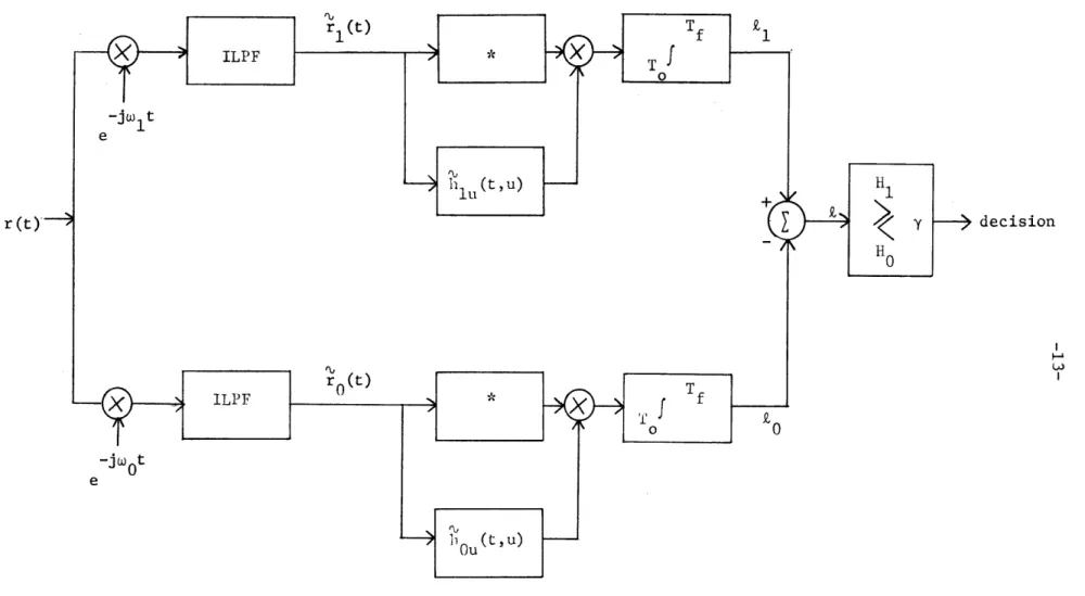
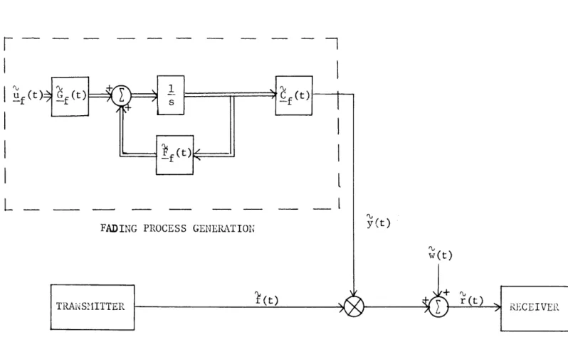
(1.14) Figure 1.1 show the optimum receiver for the binary detection problem of (1.9) as an unrealizable estimator-correlator; the block ILPF denotes an ideal lowpass filter. Figure 1.2 shows the optimum

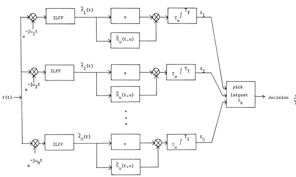
re-ceiver for the M-ary communication problem of (1.12).

Several other realizations of the operations which generate

the statistics Zk are possible. If hku(t,u) in (1.13) is factored [8]

f

S(tu) = g(x,t)g (x,u)dx, T < t,u < T (1.15)

ku T k o 0 f T then (1.13) becomes T Tf 2 Zk = gk(x,u)rk(u)du dx (1.16) T T o o

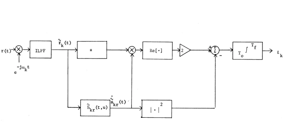
The resulting structure, shown in Figure 1.3, will be called a

filter-squarer-integrator branch. Whenever Skr(t), the

minimum-mean-square-error realizable estimate of the signal sk(t), is available, the Rk

can be generated as shown in Figure 1.4 [8-10]. The realizable filter

hkr(t,u) produces the estimate skr(t) from rk(t ) .

In order to find the configurations of Figures 1.1 - 1.3,

one of the integral equations (1.14) or (1.15) must be solved. In

Figure 1.1. Complex representation nf the estimator-correlator version of the optimum receiver for detecting Gaussian signals in white Gaussian noise.

r (t decision

I L

Figure 1.2. Complex version of the optimum receiver for M-ary communication with orthogonal Gaussian signals.

r (t) decision

7 7ý -77.ý 7

-r (t)

-3•kt

e

Figure 1.3. Complex version of the kth branch of the optimum receiver, filter-squarer-integrator realization.

·-- -

r

(t

k

3'

I

_

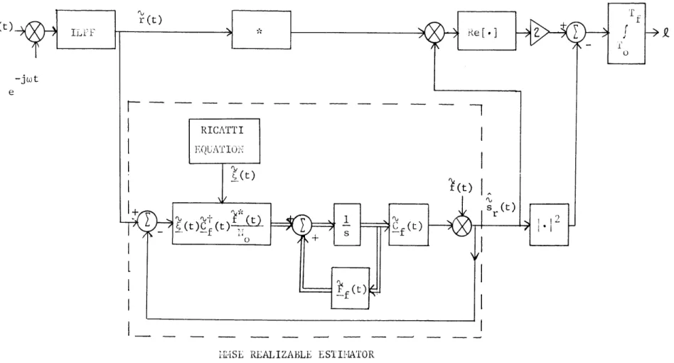
Figure 1.4. Complex representation of a realizable structure for generating the optimum £k"

-general this is difficult. Several special cases which have solutions arise when the covariance functions K% (t,u) satisfy a

"low-energy-s_k

coherence" condition [2,7,8], or are separable [8], or when the Sk(t)

are stationary and the observation interval is long [8]. The structure

of Figure 1.4 can be realized for a considerably wider class of prob-lems: whenever the processes Sk(t) have finite state representations [8,15,20].

Several measures of the performance of the optimum receiver for the binary detection problem of (1.1) have seen use [2,11,12]. A popular one is the output "signal-to-noise" ratio of the detector, but it is strictly valid only under low-energy-coherence conditions

[2,7]. Collins [13,14] has derived asymptotic expressions for the

detecLion error probabilities, Pr(EIH1) and Pr(EI

H

receiver in the general case. His method involves the use of tilted probability distributions, and the error probabilities are given in terms of the moment-generating function of the likelihood ratio. This function can be found for the special cases of low-energy-coherence, separable kernels, or stationary processes-long observation. When the sk(t) have state-variable representations, the moment-generating

functions can also be conveniently computed.

For the M-ary symmetric, orthogonal communication problem

of (1.12), the probability of error of the optimum receiver is not

known. Kennedy [6] has derived bounds on Pr(E) which also involve

momient-generating functions of the decision statistics Z . IWhen

M

the asvmDtotic exDressions for the error probabilities in the detection

problem can be applied to evaluate Pr(c) for the communication case. problem can be applied to evaluate Pr(E) for the cormnunication case.

-18-A special case of the Gaussian signal in Gaussian noise model which is treated in detail in this thesis arises when a known

wave-form is transmitted over a "dispersive" or "spread" channel [2,6,8,16,

17]. The transmitted signal is

j i)kt

fk(t) =/' Re[< (t)e , 0 < t < T (1.17)

An appropriate physical model for the channel is a collection of

moving point scatterers which reflect the transmitted signal. The

portion of the receiveu signal due to fk (t) is then modeled as a

random process. It is convenient to classify this type of dispersive

channel by its effect on the transmitted signal as doppler-spread, delay-spread, or doubly-spread.

The doppler-spread channel arises when the moving scatterers

are distributed over a region of space which is small, in units of

propagation time, compared to the duration of fk(t). As a result the

amplitudes of the quadrature components of the reflected fk(t) vary

randomly with time. The complex amplitude of the scattered return

can be modeled as [8]

sk(t) = fk(t)y(t) (1.18)

where y(t) is a complex Gaussian random process. The multiplicative disturbance in (1.18) causes sk(t) to exhibit time-selective fading; in the frequency domain this appears as a broadening of the spectrum

of fk(t). The doppler spread channel is also referred to as a

tuating point target model.

When the scatterers are moving at a rate which is small

com-pared with l/T, but have a spatial distribution in units of propagation time which is significant compared to T, the result is the

delay-spread channel. Here each scattering element returns fk(t) with a

random phase and amplitude which do not vary with time. Mathematically, the total return is given by

Sk(t) = k(t - X)y(X)dX (1.18)

-00

where y(X) is a complex Gaussian random process. Equation (1.18)

indi-cates that the duration of Sk(t) exceeds that of fk(t); Sk(t) also exhibits frequency-selective fading. The delay-spread channel is also called a deep or extended target model.

A combination of the effects which produce the doppler- and delay-spread models results in the doubly-spread channel model. Here each spatial element of the moving scatterer distribution acts as a point fluctuating target. The integrated return is

oo

sk(t) = k(t - A)y(A,t)dX (1.19)

-- O

where y(X,t) is a two parameter, complex Gaussian random process. The received signal exhibits both time- and frequency-selective fading in this case; both the duration and bandwidth of fk(t) are increased. The doubly-spread channel is also termed the deep fluctuating target model.

Construction of optimum receivers and evaluation of their

-2C-performance for detection or communication with the spread channel model above is feasible in certain situations. Price [1,2,7] has

considered this problem in detail when a low-energy-coherence condition

prevails. Stated briefly, this condition requires the eigenvalues of

the kernel K% (t,u) all to be much smaller than the additive white

s

k

noise spectral density, N . Physically, this means that no time

interval over which Sk(t) is significantly correlated can contain an appreciable portion of the total average received signal energy. In

this case, optimum receiver structures and performance expressions are

available. However, the most comprehensive treatment of the Gaussian

signal in Gaussian noise problem is possible only with the

state-variable techniques outlined above. For thie case of the transmission

of known signals over dispersive channels only the doppler-spread model can be solved in general, since it is possible to specify a

state-variable model for the multiplicative fading process y(t) and

hence for sk(t).

A considerable protion of this thesis is devoted to the derivation and discussion of techniques for specifying the optimum receivers for delay-spread and doubly-spread channels, and for

eval-uating their performance. These methods involve

distributed-para-meter state-variable representations for random processes. Lvaluation

of the moment-generating functions of the optimum receiver decision

statistic allows the calculation of the appropriate error probabilities.

Of the optimum receiver structures in Figures 1.1 - 1.4, the

filter-squarer-integrator of Figure 1.3 is the easiest to implement

from a practical point of view. However, the solution of (1.15) is not

knovw except in a few special cases. The filter-squarer-integrator receiver may still be used with a different filter, although it will then be no longer optimum. Its performance may not suffer much, pro-vided that the filter is chosen properly. In order to compare the optimum receiver with any supoptimum receiver, a technique for the evaluation of the suboptimum receiver error probabilities must be available.

This thesis presents a method of evaluating the detection error probabilities for any suboptimum binary receiver. The technique

is similar to that described above for the evaluation of optimum receiver error probabilities. The results are asymptotic expressions which involve the moment-generating functions of the receiver decision

statistic. For the 1,J-ary orthogonal cormmunication problem, bounds on

suboptimumi receiver error probabilities are evaluated.

The application of the expressions for the suboptimum error

probabilities depends on the ability to compute the moment-generating

functions of the suboptimum receiver decision statistic. This is done for two classes of suboptimum receivers: the filter-squarer-integrator structure and the finite quadratic form. The latter term describes a receiver with a decision statistic that can be written

N N

k = I r.W.or. (1.20)

i=i j=1

where the r. are complex Gaussian random variables [8]. The resulting

1

expressions for the receiver error probabilities are evaluated for the spread channel detection problem and compared with the optimum receiver

----

-22-performance. These comparisons provide insight into the design of suboptimum receivers and signals for the dispersive channel model.

A brief outline of the thesis follows:

Chapter II derives asymptotic expressions for the error probabilities of any suboptimum receiver used for binary detection.

Bounds are given on the probability of error for the LN-ary symmetric,

orthogonal com,,urnicatzon problemi. Moment generating functions for

optimum, filter-squarer-integrator, and finite quadratic form re-ceivers are specified for the Gaussian signal in white Gaussian noise model.

Chapter III considers the doppler-spread channel model. A

particular filter-squarer-integrator suboptimum receiver is specified

and its performance is evaluated. A second suboptimum receiver is

suggested and error probabilities for it are calculated. A compar-ison of the performance of optimum and suboptimum detectors is given.

Chapter IV treats the delay-spread channel model. The notions of time and frequency duality [6,18] are used to relate the

delay-spread model to the doppler-spread problem. An alternative

technique is established for finding the performance of the optimum receiver. Two suboptimuum receiver structures are specified and their error probabilities are evaluated using the results of Chapter II.

Chapter V presents a distributed-parameter state-variable

model for the doubly-spread channel model. A realization for the

optimum detector is given and a method for evaluating the error

Chapter VI considers two suboptimum receiver structures for the doubly-spread channel detection problem. They are related to the

suboptimura receivers treated earlier in the doppler-spread and

Uelay-spread models. A method of evaluating their performance is given. The

suboptimum receivers are compared with the optimum receiver for the same example presented in Chapter V.

Chapter VII is a summary of the results of the thesis. Some comments on signal design for dispersive channels are included. Suggestions for further research are given.

-24-CIt•PTER II

ASYMPTOTIC ERROR PROBABILITY EXPRESSIONS FOR TIHE DETECTION OF GAUSSIAN SIGNALS

IN GAUSSIAN NOISE

The problem of finding the detection error probabilities for a receiver which makes a decision by comparing a random variable with a threshold can be approached in several ways. The most direct is to find the probability density function of the decision statistic and integrate over the tails of the density to get the error probabilities. For the detection of Gaussian signals in Gaussian noise, the optimum receiver of Chapter I performs a non-linear operation on the process

r(t). In this case the probability density of the decision statistic

is not known. Even in problems where the density function is known, it may be difficult to perform analytically or numerically the inte-gration required to obtain the error probabilities.

For the Gaussian signal, binary detection problem of Chapter I, it is possible to write the optimum receiver decision statistic as an infinite, weighted sumn of squared, independent Gaussian random variables with known variances [8]

S=

.•ii

2

(2.1)

i=l

This suggests two possibilities for finding the error probabilities. The first is the application of the central limit theorem to the suns

of (2.1) to establish that Z is a Gaussian random variable. This fails because (2.1) violates a necessary condition for the use of the central

limit theorem [8]. The second approach is based upon the fact that an

expression for the characteristic function of . is available [8,13].

Inversion of the characteristic function gives the desired density func-tion, but in this case the inversion must be done numerically. This is impractical due to the form of the characteristic function and the necessity of accurately obtaining the tails of the density function [13].

Collins [13,14] has developed an alternate method of com-puting the optimum receiver error probabilities provided that the semi-invariant moment-generating function of the logarithm of the likelihood ratio is available. This technique involves the notion of tilted

probability densities and the resulting error probability expressions

are in series form. The semi-invariant moment-generating function is

closely related to the characteristic function of

Z

the Gaussian signal in Gaussian noise probleir the optimum receiver

error probabilities can be evaluated.

Essential to Collins' derivation is the fact that the receiver

is optimum: it compares the likelihood ratio with a threshold. The

discussion above on the calculation of error probabilities is relevant

also when a receiver which is not optimum is being used. This is the

case in many practical situations. Hence a generalization of Collins' results would be useful, if the moment-generation function of the out-put of this receiver is available.

-26-i(s) =

P

I

IH.],

The functions P.(s) generally exist only for some range of values of s. 1

Given H a tilted random variable O0s is defined to have a probability density function

sL-0

O(s)

P (L) = e

Os

(2.5)

P IH (L)

From (2.2) the probability of error give H0 is

Pr(EIH ) = f p (L)e y _Os

(2.6)

Thus the random variable

F, -;0(s) Os 0

is zero-mean and has a unit variance. Rewriting (2.6) in terms of the

density function p (Y) gives

(2.7)

(2.8)

1 _ _ ,, - - -

----MIn(s)-sL

----

-28-where

noting that

1O(S) - sýO(s)

-

s

s)yf

Y

Pr ( IIH) = e f e

py

P (Y) = p (Y• (s + (s))

Y -

10(S)

6 =

An upper bound on Pr(IlH0) is obtained from (2.9) by

exp(-s / (s) Y) < s > 0, Y> 0 Then if

Y 1

0(s)

(S) - S(s)

(Y)dY

f

po(S)

-

S4o(s)

(2.10)

I

_

_

, s >

, y >

o(s)

Note t1~at the bound of (2.14) is val~id for any s that satisfies the

conditions of (2.13).

If the random variable y in (2.8) is G~aussian, the evaluation

of the integral in (2.9) is straigh-tforward. Tn general y is not

Gaussian, but it is often the sum of a large number of random variables.

Thus for cases in whiich p (Y) bears some similarity to a G~aussian

density it appears reasonable to expand p (Y) in an £dgeworth series [13,21]

Py(Y) = 3(YL) - Y3 O(3)(Y) + (>y

+ _C6(YJ 1y 2

L

~(

K

0

(S32

(The superscrip~t _{(k) denotes the ktb derivative.) Introducing (2.15)}

-30-~

(s)-s0(s)

y3

34

L

10

2

I

1

6! ¥3

6

)

)

)

)

I

rapidly.

To obtain a similar series for P'r(c.J Ul a second tilted

randoml variabl~e Zl is define~d

sL-vI (s)

S(L) =

Is peji (L)

whiere i-i(s) is given by (2.4). Fromn (2.3)

Pr(Ej H) 1 = eli ) - p9 (L)dli (2.24)

With the norm~alized random variable

(2.25) (2.24) 1)econles a -sV~i7~ x

fe

An upper bound on P'r(e1H) ₁ is obt ained by noting that

exp (-

~

-32-Thus if (2.26) becomes Pr(J H H) < C Is()- siJ,(s)

f

i

i~UtC that the bound of (2.31) is valid for any s satisfying; the conditions

of (2.30).

An asymptotic expansion for P'r(EjIi1) is obtained by the samne

procedure used for Pr(Ejl l). Thie density p~()i xaddi iesre

of (2.15) and introduced into (2.26). The result is

PrEJ11 =e i(s)-sii

(s)

v

o

2

fe

i1(·]

j

The integral I_k can be expressed recursively as

k

I'

₀

₂

Ik k-1 + exp(-) (k-l)(), k > 1 (2.35)

Approximations to Pr(E_{IH 1}) are obtained by truncating the series (2.32).

Equation (2.32) is valid for any non-positive s for which p (s) and its

derivatives exist.

The error probabilitv hbounds (9 _.L-7 1 • a7d (9 3-1- _.L·JL ) n1 r fv-eb--to,_{L LI~ er-~V}

at ten tion . The constraints of (2.13) and (2.30) limit the ran~e o h

threshold y. Since U₀(s) and il(s) are variances, they are positive,

and thus the ji.(s) are monotonically increasing functions. Then the conditions (2.13) and (2.30) imply that

Y > j0(0)

_{= E[Z H}

0

O

(2.36)

Y 1(0)

= E[IHJ

]

This indicates that the threshold y must lie between the means of Z on

Hi₀ and II1 if the bounds of (2.14) and (2.31) are to be used.

The bounds on the error probabilities may be optimized by

the proper choice of s. The derivative of the exponents in each of

the bounds (2.14) and (2.31) is -sji(s). Since s is constrained to be

positive on 1H₁ and negative on Ii0, and since the

pi(s)

this implies that Isl should be made as large as possible in each case.

The conditions (2.13b) and (2.30b) limit how large Isj can be. Hence

-34-the optimized bounds are

Pr(E H I) < e 0(s0)-s0 0(s0 (2.37)

Pr(EIH 1) < e (2.38)

where so and s1 are determined by

0(So)

1 (S)

(2.39)

s > 0 , s < 0

0

1-Since the values so and sl in (2.39) optimize the bounds, they are

good candidates for use in the series expansions for the error prob-abilities.

The bounds on, and asymptotic expressions for Pr(cHll 0) and

Pr(ElH₁) given above hold for any binary receiver that compares a

random variable to a threshold. For these results to be useful, the

semi-invariant moment-generating function

pi(s)

Also convergence of the series expressions is not likely to be rapid if the tilted probability densities differ greatly from a Gaussian density. Unfortunately, little is known about the convergence of the

error probability expressions in general; see Collins [13] for a

discussion of this issue.

When the decision statistic

R

likelihood ratio, Pr(EIH1) and Pr(cjH0) are related. The connection is

established by noting that

P (RI )

Z = Zn A(r(t)) = n (2.40)

op _{p (R} 0

where R is a sufficient statistic [20] and A(r(t))is the likelihood

ratio. Then sk

P

in

f

The condition on s comes from the relation of (2.41) and the simul-taneous satisfaction of (2.11) and (2.28). Thus both of the optimum

receiver error robabilities

s

of one of the

p.(s),

threshold; usually p (s) is used [13].

B. Error Probability Bounds for l-ary Orthogonal Communication

This section evaluates upper and lower bounds on the probability of error of a receiver deciding which one of M bandpass Gaussian random processes is present. The receiver structure is similar to that shown in Figure 1.2: the complex representation of each branch is identical; only the carrier frequencies differ. It will be assumed that the k are sufficiently separated to ensure that the

-- .W ___

-36-branch outputs are independent random variables. Furthermore, it is assumed that the outputs of all the branches which have inputs con-sisting of white noise alone are identically distributed. The re-ceiver makes a decision by choosing the largest of the branch outputs, £k. Equally likely hypotheses are also assumed. Note that the re-ceiver is not necessarily optimum. This section uses the results of Section A to evaluate bounds originally established by Kennedy [6].

The probability of error is given by

Pr(e) = Pr(sIHi )

(2.42)

= 1 - Pr(£_i > all kk' k # ii Hi)

From Kennedy [6], Pr(c) may be bounded by

Pr(c) < Pr(£ < h) + M Pr(h<£ < z ) (2.43)

s - s -- n

Pr(E) > -

4

s

n

where the latter bound holds provided that

M Pr (Zn > h) < 1 (2.45)

The random variables ks and Zn are branch outputs when s(t) + w(t)and ,w(t),

respectively, are inputs. The variable h may take on different values in the two bounds.

The lower bound (2.44) is composed of factors for which expressions are available from Section A. From (2.32)

Pr(£ < h) = e s -lc

(s)-s

lc

(s)

]

Ic (s)

(s)

The semi-invariant moment-generating function for ' , the branch output

when a signal is present, is

(2.50)

Qn

Pr0(s)

- sOc (s)

J

(2.46)

(2.51)

Y

(s··i

(

)

Oc

(s)

kOc

POc(s)

Equations (2.46) and (2.51) permit evaluation of the lower bound (2.44)

and the condition (2.45). The value of h can be varied to maximize the

lower bound.

The upper bound of (2.43) is first replaced by a looser bound.

Fro.m Appendix III of Kenledy [6]

<Pr(h < _{S-- n}< Z ) = h p (Ls ) (L )dL uL S S I" t(L -L ) s n n s S T1 p0c (t) < e f p _h (L_s s

bs

)e

fp

(2.55)

_

I

-40--where T = T - T f log2 =1 R = C = a TRn 2

and k , k are constants. Er is the expected value of the received

energy in Sk(t) over the observation interval, and C is the infinite

bandwidth, additive white Gaussian noise channel capacity in bits/second.

The function E°( R ) is termed the system reliability function, and it

is discussed by Kennedy [6]. Appendix I shows that

R E (P ( ) R < R rit -- crit LO( ) =

(2.64)

where crit is determined by the equations

crit crit C (2.65)

ý1c(s)

-s11l

(s ) -Ij (-S)

R

R

1

E

_h

_C

)

_a

[s

_lc

(s)-P

_lc

(s)]

RCa

C

The

pic(s)

An expression for Pr(E) can be derived when M = 2. Then

Pr(c) = Pr(2. - k < 0 )

s n (2.68)

The semi-invariant moment-generating function of £ - Z is

s n bc (s) = kn E[ e S - £n Ebe s - n) s] + 9n E[e (2.69)

-Plc(s) + pO0c(-s)

ilc (s) = I c(-s)

-42-The asymptotic expansion for Pr(E) follows directly from (2.32)

Pr((s) -S bc(S) Pr(c) = e A bc Ik = f exp(-s j7Jbc(S)x) ( I 3 13 + ... ]

0

3--

3

L[C]s1

k

IUb c(s) 2

A bound on Pr(c) is available from (2.38)

Pr(s) < e

lbc(S)

ibc (s)

s< 0

When Hi = 2 and the optimum receiver is used, tight bounds on

Pr(F) are available from Pierce [27]. From (2.69) and (2.41)

1*bc(s)

_~cbc

where the * indicates that the optimum receiver is used. Then Pr(E)

may be bounded by [13] (2.70) (2.71) (2.72) (2.73) (2.74) (2.75)

___W

exp(*bc(-

.5))

< Pr(c) < (2.77)

2[+/.125UIbc (-.5)] - 2[+/. 125b c (-.5)]

Note that this is consistent with (2.74). Equation (2.77) indicates

that for optimum reception in the binary symmetric orthogonal

communi-cation problem, the quantity *bc (-.5) is an accurate performance

indicator.

This section has evaluated bounds on the Pr(c) for the IN-ary

communication problem of (1.12). Any receiver may be used that has

identical branch structures and statistically independent branch outputs.

The expressions given are not useful, however, unless the

moment-generating functions are available. The remainder of Chapter II considers the moment-generating functions associated with the optimum receiver and with two classes of suboptimum receivers for the Gaussian signal in white Gaussian noise model outlined in Chapter I.

C. 2ýoment-Generating Functions for Optimum Receivers

T'his section reviews the semi-invariant moment-generating functions for the optimum receivers in the detection problems (1.9) and (1.10), and t]he communication problem (1.12). These results are

Ailics i-r Crnl 1 -c Fll 21 1 T~ot--r~v F9/I1 - '11Pbc im~~1,r-C~r7 cf -i-hc rP-sulting expressions is considered for situations in which the random processes in the models have finite state-variable representations.

For the binary detection problem of (1.10) the

moment-gener-ating function for the optimum receiver decision statistic on H0 is

In

(s) = (l-s) I )n(1 + )+ s

n=l 0 n=1

n (1 + )~-

f

0 < s < 1

where the (A } , {A } , and (X } are the eigenvalues of the

in On cn

process Sl(t), s (t), and the composite process s (t):

proesss I1 o

(2.79)

Equation (2.41) gives the moment-generating function on 1•

raln i1ucino

Pl(S)

For the special case of (1.10), simple binary detection, (2.78) reduces to

n(s) = (1-s))

X

kn(1 +

N)

Here the {in} are eigenvalues of the process s(t) in (1.10).

For the

H-ary

moment-generating function of (2.54) is identical with that of (2.81)

co

*c(s) = (l-s)

I

)

1

Here the {A } are the eigenvalues of the complex process sk(t) which

n

has the same complex covariance function for all k. For the binary

symmetric communication problem (M = 2),

p*bc(s)

and (2.82) bc (S) = n(l + n -) - ,n(l-sn ) n=1 0 n=l N0 O _{(1 + s)A} - en(l + n ) (2.83) n=1 0

Closed form expressions for the moment-generating functions given above exist under certain circumstances. All of these formulas involve the Fredholm determinant associated with the random process

s(t) [22]

oo

D,(a) = H (1 + ali ) (2.84)

i=l

The {A.} are the eigenvalues of l(t,u). This function can be related

1 S

to a filtering error [8,24] Tf

ninD (a) =

r

T

o

where ý (t) is the minimum-mean-square realizable filtering error

P

obtained in estimating the random process s(t) which is imbedded in

complex white Gaussian noise of spectral density (A.

When s(t) has a finite state-variable representation, (2.85)

-46--j

can be evaluated, since t. (t,s(t),a) is available as the solution of a

P

inon-linear differential equation obtained in solving the estimation

problem [20]. A more convenient method for evaluating the Fredholm

determinant is known [10, 24]. Suppose s(t) has the complex

state-variable representation _[15] x(t) = 1(t)'(t) + (t)_(t) (2.86) s(t) = _(t)x(t) E[u(t)u (a)] = Q6(t - a) (2.87)

E['(T ) (T

_{)] =}

_P

T

where the superscripts and _{denote transpose and conjugate transpose,}

respectively. Then the Fredholm determinant for s(t) is given by

Tf

enDF ( a ) = zn det 2 (Tf) + f tr[ " (t)]dt (2.8 9)

T

where

4

equation

il~ (t) _(t) W(t)Q # r(t) •!((t)

dt- --- _(2.90)

2 (t) 2()

y .(To)

2 (To)

The functions det (.) and tr(.) are the determinant and trace, respec-tively, of their matrix arguments.

Thus either (2.85) or (2.89) provides a way to evaluate the Fredholm determinant for a wide class of signal processes. This in turn allows computation of the optimum receiver error probabilities or bounds on those probabilities.

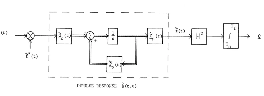
D). Uoment-Generating Functions for Filter-Squarer-Integration Receivers

This section obtains the moment-generating functions for a class of receivers which are generally suboptimum. The structure of each branch in the receivers for the binary detection problem and

,-ary communication problem of Chapter I is a linear filter followed

by a square-law device and an integrator. This

filter-squarer-integrator (FSI) receiver is shown in Figure 2.1. The filter may

ru

be time-varying. The choice of g(t,u) which makes the FSI receiver an optimum receiver is unknocwn except in a few special cases.

The moment--generating function for thie FSI receiver output statistic Y can be obtained by first writing the random process z(t)

in Fiiure 2.1 in a Karhunen-Loeve expansion: [20,22]

z(t) = z (t), T < t < T (2.92)

= n n

n=l

-jwt LINEAR

e FILTER

Figure 2.1. Complex version of the filter-squarer-integrator receiver branch.

ICII-_I^.

~-~---where S(t)~:. (t)dt = 6 '1" ''nl " o

E[z z

]

A

n

zI=

f

I

(t)l

-

r1z

I

(2.95)

.ience Z is the sum of the squares of statistically independent, complex

Gaussian random variables [8], with variances given by (2.94). The

moment-generating function of Z under H. is

1

n

Lie

)

, 2 l n I £n E[ e I H_{i ]} n=l = - E zn(1 - sAin) (2.96) n=l (2.93) Then (2.94) ... mm _Y z On z pin m (t)!,U •m(t))dt

-50-by (9.d7) of [22]. T;e first {(. } are the eigenvalues of Z(t)

,iven that 1. is true. Equation (2.96) is valid for

1

(2.97)

s < i ax { in }

-For the simple binary detection problem of (l.10), the

(2.4 ) follow directly from (2.96)

p₀(s) = -n=1

1

₁

(S)

=

The X On} and the {ln} are the eigenvalues of z(t) in Figure 2.1

when r(t) = (t) and (t) = s(t) + w(t), respectively, are inputs.

For the general binary problem of (1.9) with branch outputs l and k0

which are independent, the

p.i(s)

1

an (1 - slo

-

X

pl(s)

=

The

xi

jn J 1

For the M-ary communication problem of (1.12),

pOc(s)

UlC(S) in (2.54) and (2.50) are identical to

p

respec-tmVely, given by (2.98) and (2.99). When i = 2, bc() in (2.69) is

p

(s) of

P

(s) =

Sbc(s) = - I nn(1-sAln) - I Zn(l + sXOn (2.102)

n=1 n=l1

The moment-generating functions (2.98 -2.102) can all be

expressed in terms of Fredholm determinants, (2.84). The previous

section indicated that computation of DF(a) is feasible whenever the

{A }i of DF(a) are eigenvalues of a state representable process. In

the case of the FSI receiver, then, the error probability expressions

can be conveniently computed when z(t) in Figure 2.1 has a finite

state representation. For this to happen, both r(t) and the filter g(t,u) should have state-variable representations.

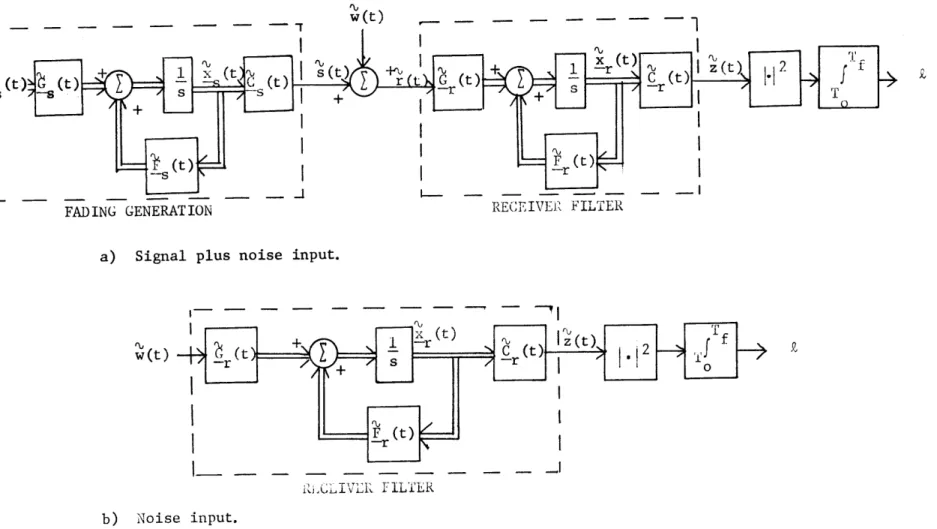
Figure 2.2 shows a model in which the filter in the FSI receiver has a finite number of states and the signal s(t) is re-presented as the output of a finite state system driven by white noise. Figure 2.2a is the model when the receiver input is signal plus noise. The signal state equations are

x (t) = - (t) (t) + (t)u (t) -s -S -S -s -S (2.103) s(t) = (t) x , (t) -S S E[us (t) (o)] = s6(t - o) (2.104)

L[x (T )x(T

)]

= P

and those for the receiver

I-- - - - - -

-1%S

I

I

a) Signal plus noise input.

- - -

T

Figure 2.2. Comiplex state-variable model for the detection of a Gaussian signal in white

Gaussian noise with a filter-sqluarer-integrator receiver.

S _{(t) = F(t)x (t) + G (t)r(t)}

-r -r ---r

(2.105)

E [r (T o) (T) ] --or (2.106)

The receiver initial condition P is arbitrary. A composite

state--or

variable model for the system of Figure 2.2a can be defined by letting

-_s (t) = (2.107a) x (t) (t) 0

t](t)

=

(2.107b)

L

G (t)

UP

0

Q

=

(2.107d)

•(t)

i·

---

~-

-- -54-,ýI u(t) = (2.107f) --os SorJ

Equations (2.84 - 2.91) can be used directly to give the Fredholm

determinant for the model above. This in turn provides a means of

obtaining u_(s) in (2.99).

When the input to the FSI is just Iw(t), the model of Figure

2.2b is appropriate. The system of differential equations is defined

by letting x(t) = (t) 14r -r =

'

Again the results of the previous section provide the Fredholm

deter-minant for z(t) when noise alone is the input to the FSI receiver;

then (2.98) follows immediately. The rest of the moment-generating

functions of this section can then be expressed in terms of (2.98) and (2.99).

Although it is necessary that both the signal s(t) and the receiver filter have state-variable representations for easy compu-tation of the Fredholm determinant, a wide class of signals and filters

fall into this category. Once the semi-invariant moment-generating functions are available for the FSI receivers, the error probabilities can be calculated. The resulting suboptimum performances can be

compared with the optimum.

E. Moment-Generating Functions for Quadratic Forms

In the following chapters another receiver which is generally suboptimum will be considered. It is one composed of branches with outputs that can be written as finite quadratic forms

N N

L= r. (2.109)

i=l j=1

The {ri.} are complex Gaussian random variables ( see [8] for details).

1

If a vector and Hermetian matrix W are defined

r

= * (2.110)

r_N

-56-then

R

= R P, (2.112)

An example of a receiver with this decision statistic is one in which r(t) is passed into a bank of linear filters. The sampled filter outputs, ri, are quadratically combined, as in (2.109). This

type of receiver will be considered in the following cliapters. The

optimum receiver for a diversity commiunication system operating over a Rayleigh fading channel is another case in which the operation of

(2.109) appears.

The momennt-generating functions of £ can be found by first defining the conditional covariance matrices

A = E[' AI Isignal + noise ] (2.113)

--s

A = E[ noise] (2.114)

where the conditions refer to the branch input. The joint probability

density function for

i

)

= exp{ -

m

where the

I

means determinant. Then

where the notation 1-1 means determinant. Then

P0(s) = en E[e se noise]

-A

(2.98) and (2.99) for simple binary detection. Equations (2.100 - 2.102)

for the other cases follow directly. Thus the error probabilities for another class of generally suboptimum receivers can be evaluated,

pro-vied that the matrices A, A , and A in (2.118) and (2.119) are -S -I known.

__---4

f

--

-1

PO(S) = -en det(I - s A ) (2.118)

and correspondingly

Pl (s) = -en det (I - s

ls

The expressions of (2.118) and (2.119) can be used in place of

-58-F. Summary

This chapter has considered methods of computing error prob-abilities for receivers which use a threshold comparison to make a binary decision. A technique for evaluating the error probabilities is derived which depends on the knowledge of the semi-invariant rmoment-generating function of the decision statistic. The derivation uses tilted probability densities and is similar to one devised previously for optimum receivers. The asymptotic expressions for the error probabilities are also used to evaluate error probability bounds for an .1-ary communication problem.

The case of the detection of Gaussian signals in Gaussian noise is considered next. Moment-generating functions for the optimum

receiver are reviewed, as well as an efficient technique for computing them when finite state-variable models are available for the received

signal processes. "Moment-generating functions for two classes of generally

suboptimum receivers are derived: filter-squarer-integrator receivers and quadratic form receivers. The moment-generating functions of the

first class can be conveniently computed if the receiver filter has finite state representation. The error probabilities of the optimum and suboptimum receivers can then be compared.

The following chapter considers a particular example of the

Gaussian signal in Gaussian noise model: the reception of known signals

transmitted over a doppler-spread channel. Since a state-variable

representation is available for the signals in this model, it is

possible to directly apply the results of this chapter. The

Elance. Insight into the design of signals and suboptinimu

w.ill be provided by numerical examples. 'Ihe delay-spread and

CHAPTEI'I III

DETECTIOAN OF KNOWN SIGNiALS T.RA1SH;ITIED OVER DOPPLER-SPREAD CiHANNELS

This chapter considers the problem of detecting known signals which are transmitted over doppler-spread dispersive channels. This problem is I special case of the Gaussian signal in Gaussian noise

detection problem of Chapter I. The results of Chapter II can be

applied here if a state-variable model for the doppler-spread channel is available. Such a model is specified, and the performance of the

optimum receiver and several suboptimum receivers is analyzed. The first section gives a model for the doppler-spread

channel. Implementation and the performance of the optimum receiver is reviewed. Filter-squarer-integrator (FSI) suboptimum receivers are dis-cussed. A particular FSI configuration is chosen, and the results of Chapter II are used to evaluate its performance. A second suboptimum structure, called a correlator-squarer-sum (CSS) receiver, is suggested. Its performance is analyzed and is compared to that of the optimum and FSI receivers for a variety of signal and channel parameters.

A. The Doppler-Spread Channel Model

The doppler-spread channel model considered here can be

de-rived [6,8] by assuming that a narrowband transmitted signal

f(t) = /Y Rc[r(t) e jt], 0 < t < T (3.1)

is reflected by a collection of moving point scatterers. The dimensions of the spatial distribution of the scatterers are small, in units of propagation time, compared to the transmitted signal duration T. It can be shown [6] that the random movement of the scatters produces a

fluctuation in the amplitudes of the quadrature components of ?(t). In

terms of complex amplitudes, a suitable model for the scattered return in white noise is then

r(t) = (t)y(t) + w(t)

= s(t) + w(t) 0 < t < T (3.2)

The multiplicative disturbance y(t) is a complex Gaussian random process. Any pure delay or doppler shift in the channel is assumed to be known

and therefore is not included in the formulation of (3.2). The

ob-servation interval in (3.2) takes into account that the only interval

during which a scattered return may be present is [0,T]. This model

is also known as a fluctuating point target model [2,7,8,16].

The multiplicative fading process y(t) will be assumed to be zero-mean and have the known covariance function

E[y(t)y (u)] = ý(tu) (3.3)

y

Then the covariance function for the signal component s(t) is

dn. (\. f\, .3

K%(t,u) = f(t) im(t,u)f (u) (3.4)

sy

Tile energy in the transmitted signal •(t) is

2!c(t) t AE (3.5)

-62-The expected value of the received energy in s(t) is

Tf

T

E[ f I

(t)l2 dt

]

E[

f

f(t)1

K,(t,t)dt]

A

= E

The zero-mean, additive white noise w(t) has the covariance function

E[w(t)w (u)] = N 6(t-u)

o

The model above has a convenient state-variable description whenever the fading process y(t) has a state-variable representation. Suppose y(t) is the output of a linear system driven by white noise

Xf(t) = _f(t) , (t) + ýf(t) uf(t)

(3.8)

y(t) = wf(t) xf(t)

E[uf (t) f(a)] = Cqf t-G)

(3.9)

Then the signal s(t) is described by the model of (2.86 - 2.88) if

-f F(t)=

i~f(t)

I

_y

Vhen y(t) is a stationary random process, the channel

is a special case of the "wide-sense stationary uncorrelated scatterer"

(WSSUS) channel model [6,8,16] that will be discussed in Chapter V. In

this case the covariance function of y(t) is written Kv(t-u), and the

matrices _f(t), Cf(t) and C•(t) in (3.10) are all constant. Also

(3.6) reduces to

L

=

K

(0)

f

(f(t)I

dt

(3.11)

where P is the average power in y(t). Although y(t) is stationary, the

process s(t) is still non-stationary, in general.

The examples that follow is this chapter are limited to the

case of stationary fading. First and second order state-variable models

are used for the numerical results. The model of (3.8) for the first

order case is f(t = -kI , k1 > 0 (t) = (t) = 1

f

f

The constant kl is chosen to be real since any imaginary part would

represent a pure doppler shift [8]. For the second order model

r

-i---7

Kft

Figure 3.1. A complex state-variable model for the bandpass doppler-spread channel.

Js

--- il-s~ --- - ~--·P~CPT'~'--L"la~ii~ ___ _ _ ---- · -·-· --u (t

L