Properties and geoeffectiveness of magnetic clouds in the rising, maximum and early declining phases of solar cycle 23

HAL Id: hal-00317575

https://hal.archives-ouvertes.fr/hal-00317575

Submitted on 28 Feb 2005

HAL is a multi-disciplinary open access

archive for the deposit and dissemination of

sci-entific research documents, whether they are

pub-lished or not. The documents may come from

teaching and research institutions in France or

abroad, or from public or private research centers.

L’archive ouverte pluridisciplinaire HAL, est

destinée au dépôt et à la diffusion de documents

scientifiques de niveau recherche, publiés ou non,

émanant des établissements d’enseignement et de

recherche français ou étrangers, des laboratoires

publics ou privés.

the rising, maximum and early declining phases of solar

cycle 23

K. E. J. Huttunen, R. Schwenn, V. Bothmer, H. E. J. Koskinen

To cite this version:

K. E. J. Huttunen, R. Schwenn, V. Bothmer, H. E. J. Koskinen. Properties and geoeffectiveness

of magnetic clouds in the rising, maximum and early declining phases of solar cycle 23. Annales

Geophysicae, European Geosciences Union, 2005, 23 (2), pp.625-641. �hal-00317575�

SRef-ID: 1432-0576/ag/2005-23-625 © European Geosciences Union 2005

Annales

Geophysicae

Properties and geoeffectiveness of magnetic clouds in the rising,

maximum and early declining phases of solar cycle 23

K. E. J. Huttunen1, R. Schwenn2, V. Bothmer2, and H. E. J. Koskinen1,3

1_{Department of Physical Sciences, Theoretical Physics Division, P.O. Box 64, FIN-00014 University of Helsinki, Finland} 2_{Max-Planck-Institut f¨ur Sonnensystemforschung, D-37191, Germany}

3_{Finnish Meteorological Institute, P.O. Box 503, 00101 Helsinki, Finland}

Received: 30 March 2004 – Revised: 1 October 2004 – Accepted: 12 October 2004 – Published: 28 February 2005

Abstract. The magnetic structure and geomagnetic response

of 73 magnetic clouds (MC) observed by the WIND and ACE satellites in solar cycle 23 are examined. The results have been compared with the surveys from the previous solar cy-cles. The preselected candidate MC events were investigated using the minimum variance analysis to determine if they have a flux-rope structure and to obtain the estimation for the axial orientation (θC, φC). Depending on the calculated

inclination relative to the ecliptic we divided MCs into “bipo-lar” (θC<45◦) and “unipolar” (θC>45◦). The number of

ob-served MCs was largest in the early rising phase, although the halo CME rate was still low. It is likely that near solar maximum we did not identify all MCs at 1 AU, as they were crossed far from the axis or they had interacted strongly with the ambient solar wind or with other CMEs. The occurrence rate of MCs at 1 AU is also modified by the migration of the filament sites on the Sun towards the poles near solar maxi-mum and by the deflection of CMEs towards the equator due to the fast solar wind flow from large polar coronal holes near solar minimum. In the rising phase nearly all bipolar MCs were associated with the rotation of the magnetic field from the south at the leading edge to the north at the trailing edge. The results for solar cycles 21–22 showed that the direction of the magnetic field in the leading portion of the MC starts to reverse at solar maximum. At solar maximum and in the declining phase (2000–2003) we observed several MCs with the rotation from the north to the south. We observed unipo-lar (i.e. highly inclined) MCs frequently during the whole investigated period. For solar cycles 21–22 the majority of MCs identified in the rising phase were bipolar while in the declining phase most MCs were unipolar. The geomagnetic response of a given MC depends greatly on its magnetic structure and the orientation of the sheath fields. For each event we distinguished the effect of the sheath fields and the MC fields. All unipolar MCs with magnetic field southward at the axis were geoeffective (Dst<−50 nT) while those with

Correspondence to: K. E. J. Huttunen

(emilia.huttunen@helsinki.fi)

the field pointing northward did not cause magnetic storms at all. About half of the all identified MCs were not geoffective or the sheath fields preceding the MC caused the storm. MCs caused more intense magnetic storms (Dst<−100 nT) than

moderate magnetic storms (−50 nT ≥Dst≥−100 nT).

Key words. Interplanetary physics (Interplanetary

mag-netic fields) – Magnetospheric physics (Solar wind-magnetosphere interactions) – Solar physics, astrophysics and astronomy (Flares and mass ejections)

1 Introduction

Manifestations of coronal mass ejections (CMEs) are fre-quently observed in the solar wind near 1 AU and are com-monly called interplanetary coronal mass ejections (ICMEs). The term magnetic cloud (MC) is used to characterize an ICME having a specific configuration in which the magnetic field strength is higher than the average, the magnetic field di-rection rotates smoothly through a large angle, and the proton temperature is low, Burlaga et al. (1981); Klein and Burlaga (1982); Gosling (1990). Because of the high magnetic field strength and low proton temperatures MCs have values of plasma beta significantly lower than 1. Near 1 AU MCs have enormous radial sizes (0.28 AU), with an average duration of 27 h, an average peak magnetic field strength of ∼18 nT and the average solar wind speed 420 km/s, Klein and Burlaga (1982); Lepping and Berdichevsky (2000). The expansion of a MC produces strongly decreasing density and temperature with the radial distance from the Sun and declining profiles of speed, magnetic field and pressure, Burlaga and Behannon (1982); Gosling (1990); Bothmer and Schwenn (1998). The interaction with the ambient solar wind may prevent the ex-pansion that leads to a smaller diameter and larger densities and temperatures at 1 AU than in an average MC. Goldstein (1983) first suggested that MCs are force-free magnetic field configurations (∇×B=α(r)B).

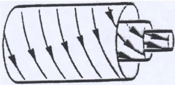
Fig. 1. The flux rope of type SWN showing the rotation of the

magnetic field vector from the south to the west at the MC-axis and finally to the north at the trailing edge of the MC (Bothmer and Rust, 1997).

A few years later Burlaga (1988) showed that a constant

αdescribes satisfactorily the magnetic field changes when a MC moves past a spacecraft. The constant α solution for a cylindrical symmetric force-free equation was given by Lundquist (1950):

BR=0, BA=B0J0(αr), BT =H B0J1(αr), (1)

where BR, BA and BT are the radial, axial and tangential

components of the magnetic field. B0is the maximum of the

magnetic field strength, r is the radial distance from the axis,

αis a constant related to the size of a flux rope, J0and J1are

Bessel functions and H =±1 defines the sign of the magnetic helicity Els¨asser (1958); Berger and Field (1984).

The four possible flux-rope configurations, as predicted from Eq. (1), have been confirmed to occur in the solar wind, Bothmer and Schwenn (1994); Bothmer and Schwenn (1998). The axis of an MC (φC, θC) can have any

orien-tation with respect to the ecliptic plane and depending on the observed directions of the magnetic field at the front boundary, at the axis and at the end boundary eight flux rope categories are often used to classify MCs, Bothmer and Schwenn (1994); Bothmer and Schwenn (1998); Mulligan et al. (1998):

– Bipolar MCs (low inclination), θC<45◦: Following the

terminology by Mulligan et al. (1998) the MCs with the axis lying near the ecliptic plane are called bipo-lar, as the Z component of the terrestrial magnetic field changes sign during the passage of an MC. Figure 1, adopted from Bothmer and Rust (1997), shows a sketch of the flux rope category called SWN. In the SWN-type MC the magnetic field vector rotates from the south (S) at the leading edge to the north (N) at the trailing edge, being westward (W) at the axis. Similarly, the three other categories are SEN (E=east), NES and NWS.

– Unipolar MCs (high inclination), θC>45◦: The MCs

that have the axis highly inclined to the ecliptic are called unipolar, as the Z-component has the same sign during the MC. The magnetic field is observed to ro-tate from the west (east) at the leading edge to the east

(west) at the trailing edge, pointing either south or north at the axis. These changes correspond to the flux-rope types: WNE, ESW, ENW and WSE.

When viewed by an observer looking towards the Sun (posi-tive axis direction) the counterclockwise magnetic field ro-tation is defined as right-handed (SWN, NES, ENW and WSE types) and the clockwise rotation as left-handed (NWS, SEN, WNE, and ESW types). The handedness can be de-termined from the parameters H and φc with the formula, C=sgn(sin φc)×H, such that C=−1 is for a left-handed MC

and C=+1 is for a right-handed MC (Lynch et al., 2003). The studies of MCs during different activity phases for so-lar cycles 21–22 revealed systematic variations in the pre-ferred flux rope types, Bothmer and Rust (1997); Bothmer and Schwenn (1998); Mulligan et al. (1998): In the rising phase of odd (even) solar cycles the magnetic field in MCs rotates predominantly from the south to the north (from the north to the south) and during the years of high solar activ-ity both SN and NS type MCs are observed. Additionally, Mulligan et al. (1998) found for the years 1979–1988 that unipolar MCs were most frequently observed in the declin-ing phase of the solar activity cycle. At solar minimum and in the rising phase most MCs were bipolar.

MCs have been studied intensively since their discovery, as they are important drivers of magnetic storms, e.g. Tsuru-tani et al. (1988); Zhang et al. (1988); Gosling et al. (1991). A magnetic storm is defined as a world wide depression in the horizantal component of the magnetic field that is caused by the enhanced ring current (Gonzalez et al., 1994). The variations in the ring current are recorded by the 1-h Dst

in-dex, e.g. Mayaud (1980). The key parameters that control the solar wind magnetospheric coupling are the strength and the direction of the interplanetary magnetic field (IMF). For ex-ample, intense magnetic storms (Dst<−100 nT) are caused

by an IMF southward component stronger than 10 nT at least for 3 h (Gonzalez and Tsurutani, 1987). Solar wind speed and density also play a role in a formation of the ring cur-rent, though their exact role is still controversial, Gonzalez and Tsurutani (1987); Fenrich and Luhmann (1998); Wang et al. (2003a). The geomagnetic response of a certain MC depends greatly on its flux-rope structure, e.g. Zhang et al. (1988); Bothmer (2003). In some cases MCs cause major magnetic storms, for example, Bastille day storm on 15–16 June 2000 (Lepping et al., 2001) while in other cases the magnetic field remains mainly northward during the MC and no geomagnetic activity follows. A magnetic storm can also be caused by the sheath of heated and compressed solar wind plasma piled up in front of the CME ejecta (Tsurutani et al., 1988).

In this study we have performed the first extensive survey of the magnetic structure and the geomagnetic response of MCs identified during solar cycle 23. The investigated pe-riod covers the rising phase of solar activity (1997–1999), solar maximum (2000) and the early declining phase (2001– 2003) when defined by the yearly sunspot number. The pur-pose of this study is to examine whether the variations of the

magnetic structure of MCs with solar activity found for the previous solar cycles (21–22) hold true also for solar cycle 23. During the investigated period we have continuous solar wind measurements at 1 AU from WIND and ACE space-craft, providing a larger set of MCs than was available for the previous solar cycles. We also present a detailed analysis of the geomagnetic response of the MCs, distinguishing the effect of sheath fields and MC fields as a storm drivers. The properties of MCs during solar cycle 23 have been surveyed by Lynch et al. (2003) and Wu et al. (2003). The Lynch et al. (2003) study covers only a three and one-half year pe-riod and concentrates on the plasma composition of MCs. The Wu et al. (2003) paper shortly summarizes the occur-rence rate and geoeffects of MCs reported in the WIND list at http://lepmfi.gsfc.nasa.gov/mfi/mag cloud pub1.html. In Sect. 2 we present the method to identify MCs from the solar wind data and how the axial orientation was estimated. In Sect. 3 we show statistical results and in Sect. 4 we discuss the geoeffectiveness of MCs. In Sects. 5 and 6 we discuss and summarize the results.

2 Identification of MCs and determination of their flux-rope type

We have identified MCs using magnetic field and plasma measurements from WIND (January 1997–February 1998) and ACE (March 1998–December 2003). We first performed a visual inspection of the data to find the candidate MCs. The intervals of bidrectional streaming of solar wind suprather-mal electrons (BDE) along magnetic field lines is often used to identify MCs, as this feature is considered to represent a closed magnetic field configuration (Bame et al., 1981; Gosling, 1990). However, as the interpretation of the BDE intervals is not unambiguous and BDE are present also in ICMEs without the MC structure, we did not use them as a MC signature. In this study the criteria to define an MC is based on the smoothness of the rotation in the magnetic field direction confined to one plane (see below). Additionally, we required that an MC must have the average values of plasma beta less than 0.5, the maximum value of the magnetic field at least 8 nT and the duration at least 6 h. With the last two criteria we wanted to remove the ambiguity in identifying small and weak MCs. As a consequence, we are likely to miss MCs that have been crossed far from the axis. There is often a disagreement in the number of MCs identified in dif-ferent studies because there is no unique and fully objective way to identify an MC in the solar wind (discussion, for ex-ample, in a poster by Shinde et al. at the fall AGU meeting, 2003).

All selected events were investigated by analyzing 1-h magnetic field data with the minimum variance analysis (MVA) (Sonnerup and Cahill, 1967), where MCs are iden-tified from the smooth rotation of the magnetic field vector in the plane of the maximum variance (Klein and Burlaga, 1982). For MCs with durations of 12 h or less we performed MVA using 5-min (WIND) or 4-min (ACE) averaged data.

The detailed description of the method is found in the ap-pendix of Bothmer and Schwenn (1998). The MVA method can be applied satisfyingly to the directional changes of the magnetic field vector exceeding ∼30◦. The large ratio of the intermediate eigenvalue λ2to the minimum eigenvalue λ3

in-dicates that the eigenvectors are well defined. We required that λ2/λ3 is greater than 2, based on the analysis of

Lep-ping and Behannon (1980). B_X∗, B_Y∗, and B_Z∗ correspond to the magnetic field components in the directions of maximum, intermediate and minimum variance. The MVA analysis pro-vides us with the estimation of the orientation of the MC axis (φC, θC). θ and φ are the latitudinal and longitudinal

an-gels of the magnetic field vector in solar ecliptic coordinates;

θ=90◦is defined northward and φ=90◦is defined eastward. The MC axis orientation corresponds to the direction of the intermediate variance that is seen from Eq. (1) as the axial component is zero at the boundaries of the MC. The radial component corresponds to the minimum variance direction and the azimuthal component corresponds to the maximum variance direction. The boundaries of MCs were determined by solar wind signatures (start of the smooth rotation of the magnetic field vector, drop in plasma beta, and plasma and field discontinuities) and by the eigenvalue ratio. In those cases where the boundaries defined by the different signa-tures disagreed we used the magnetic field rotation.

There are various other methods to model MCs. Lepping et al. (1990) have developed an algorithm to fit the magnetic field data to the Lundquist solution that reproduces well the observed directional changes of the magnetic field but often the magnetic field strength profile is not so well fitted. To improve the results the kinematic effects, such as the expan-sion and the assumptions of non-symmetric and non-force free topologies are used in some models, e.g. Farrugia et al. (1993); Marubashi (1997); Osherovich and Burlaga (1997); Mulligan and Russell (2001); Hidalgo et al. (2002a); Hidalgo et al. (2002b).

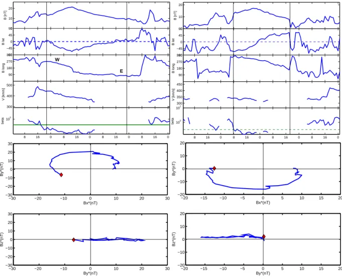
Figure 2 shows 1-h solar wind data and the calculated plasma beta during two MCs, one having the axis perpen-dicular to the ecliptic plane (left) and the other lying near the ecliptic plane (right). The bottom part of Fig. 2 shows the rotation of the magnetic field vector in the plane of maxi-mum variance and in the plane of minimaxi-mum variance. Both MCs are easily identified by the smooth rotation of the mag-netic field direction, enhanced magmag-netic field magnitude and low plasma beta. The unipolar MC was observed by ACE on 19–21 March 2001. As seen from the Fig. 2 this MC has a flux-rope type WSE and the observed angular variation of the magnetic field is left-handed. The MVA method gives the eigenvalue ratio λ2/λ3=52, the angle between the first and

the last magnetic field vectors χ =157◦, and the orientation of the axis (φC, θC)=(133◦, −57◦). The Bzcomponent was

southward almost during the whole passage of the MC (it caused a magnetic storm with the Dst minimum −165 nT).

The bipolar MC in Fig. 2 was observed by ACE on 20–21 August 1998. It belongs to flux rope category SWN and is right-handed. The MVA method gives the eigenvalue ratio 30, χ =177◦, and the orientation of the axis (φC, θC)=(113◦,

0 10 20 B [nT] −90 −45 0 45 90 B lat 90 180 270 360 B long 300 400 500 V [km/s] UT [hours] 8 16 0 8 16 0 8 16 0 8 16 0 100 beta W E 0 10 20 B [nT] −90 −45 0 45 90 B lat 90 180 270 360 B long 300 350 400 450 V [km/s] UT [hours] 8 16 0 8 16 0 8 16 0 8 16 0 100 102 beta −30 −20 −10 0 10 20 30 −30 −20 −10 0 10 20 30 Bx*(nT) By*(nT) −30 −20 −10 0 10 20 30 −30 −20 −10 0 10 20 30 By*(nT) Bz*(nT) −20 −15 −10 −5 0 5 10 15 20 −20 −10 0 10 20 Bx*(nT) By*(nT) −20 −15 −10 −5 0 5 10 15 20 −20 −10 0 10 20 By*(nT) Bz*(nT)

Fig. 2. Top part: Solar wind parameters during two MC events. Top to bottom: magnetic field strength, polar (Blat) and azimuthal (Blong)

angles of the magnetic field vector in GSE coordinate system, solar wind speed and plasma beta. Left: 19–22 March 2001. Right: 19–22 August 1998. Two solid lines indicate the interval of an MC. Bottom part: the rotation of the magnetic field vector in the plane of maximum variance and in the plane of minimum variance. The diamond indicates the start of the rotation.

−16◦). For both MCs the hodograms show that in the plane of maximum variance the magnetic field rotates smoothly through a large angle and in the plane of minimum vari-ance the magnetic field decreases/increases from about zero to the minimum/maximum value of the B_Y∗-component and then goes back to zero.

3 Statistical results on MCs

We have compared our statistical results to the results ob-tained in several other studies during solar cycle 23 and the previous solar cycles. The article, the period of the inves-tigation, duration of the study in years (T), spacecraft used (S/C), and the total number of identified MCs are summa-rized in the Table 1. Bothmer and Rust (1997) and Bothmer and Schwenn (1998) identified MCs based on the minimum variance analysis, Mulligan et al. (1998) identified and classi-fied MCs using the visual inspection of the data while Lynch

et al. (2003) and Wu et al. (2003)/WIND list used the least-square fitting routine by Lepping et al. (1990).

3.1 Magnetic cloud list

Table 2 presents the 73 MCs that we have identified from ACE and WIND solar wind data during the seven-year pe-riod (1997–2003). We have also included seven “cloud can-didate” events for which the fitting with MVA was not suc-cessful (e.g. the eigenvalue ratio <2 or the directional change less than 30◦) or that had large values of beta throughout the event. For example, 24–25 November 2001 and 23–24 May 2003 events exhibited very low plasma beta, but the orga-nized rotation of the magnetic field was not observed. For the first event the complex magnetic structure probably re-sults from the interaction of multiple fast halo CMEs that were detected by LASCO within a short time interval, Hut-tunen et al. (2002b); Wang et al. (2003b).

Table 1. Summary of the five previous studies we have compared our statistical results. In Bothmer and Rust (1997) no duty cycle

consid-erations are made. In Bothmer and Schwenn (1998) MCs were observed between 0.3–1 AU. The Wu et al. (2003) study covered the years 1996–2001. For 1995 and 2002 see the WIND magnetic cloud list.

study period T S/C MC

Bothmer and Rust (1997) 1965–1993 28 OMNI-data base 67 Bothmer and Schwenn (1998) December 1974–July 1981 6.7 Helios 1/2 45 Mulligan et al. (1998) 1979–1988 10 Pioneer Venus Orbiter 61 Lynch et al. (2003) February 1998–July 2001 3.5 ACE 56 Wu et al. (2003)/WIND list 1995–2002 8 WIND 71

1995 1996 1997 1998 1999 2000 2001 2002 2003 0 5 10 15 20 N 1995 1996 1997 1998 1999 2000 2001 2002 2003 0 50 100 150 200 SN number 1995 1996 1997 1998 1999 2000 2001 2002 2003 0 5 10 15 20 N 1995 1996 1997 1998 1999 2000 2001 2002 2003 0 5 10 15 20 N 1995 1996 1997 1998 1999 2000 2001 2002 2003 0 100 200 CMEs 1986 1987 1988 1979 1980 1981 1982 1983 1984 1985 0 5 10 15 20 N 1986 1987 1988 1979 1980 1981 1982 1983 1984 1985 0 50 100 150 200 SN number (a) (b) (c) (d) (e)

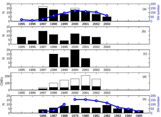
Fig. 3. Yearly number of observed MCs in our study (a), in Wu et al. (2003)/WIND list (b), and in Lynch et al. (2003) (c), the yearly number

of departed full halo CMEs (black) and partial halo CMEs (white) (d), and yearly number of MCs given in Mulligan et al. (1998) (e). Note that in Lynch et al. (2003) the year 2001 presents only 7 months data of (January–July). The circles show the yearly sunspot number. The white portion in bars in (a) show the number of cloud candidate events. In (e) the years have been arranged to coincide with the years of approximately the same solar cycle phase in (a)–(d).

3.2 Yearly magnetic cloud rate

The histograms in Fig. 3 display the yearly number of MCs identified in our study (Fig. 3a), in Wu et al. (2003)/WIND list (Fig. 3b), and given in Lynch et al. (2003) (Fig. 3c). The circles show the yearly sunspot number and in Fig. 3a the white portions in bars show the “cloud candidate” events. The fourth Fig. 3d shows the yearly number of full (an-gular width=360◦) and partial (angular width >120◦) halo CMEs as reported in the LASCO coronal mass ejection cat-alogue (http://cdaw.gsfc.nasa.gov/CME list). We have not made analysis as to whether these CMEs were front- or back-side, but numbers shown give a rough estimate of the yearly changes in the number of CMEs that can encounter the Earth. Figure 3e shows the yearly number of MCs in Mulligan et al.

(1998). Note that in Fig. 3e we have arranged the time axis so that the years corresponding to about the same solar cy-cle phase coincide between Mulligan et al. (1998) and other studies.

Figure 3a shows that we identified the largest number of MCs (15) just after solar minimum in 1997. The number of MCs was also high (13) in 1998 but there was a reduc-tion to eight MCs in 1999. During solar maximum period (2000–2001) the MC rate was high, after which the number of identified MCs decreased. The yearly numbers given by Wu et al. (2003) show a similar trend. In 1999 they identified only four MCs.

T ab le 2. MCs and clou d cand idate ev ents id entifie d in WI ND (Ja nuary 1 997–F ebrua ry 1998 ) and A C E (Ma rch 199 8–Dec embe r 2003) d ata. The colum ns fro m the left to the right g iv e: y ear , shock time (UT), M C sta rt tim e (UT ), MC end time (U T), “Q ” den otes w hethe r the ev ent w as an MC (1) or cloud cand idate (cl), in ferred flux -rope type , h anded ness of the cloud (LH= left-ha nded, R H=rig ht-han ded), dir ection of the M C axis (φ C , θC ), eig en v alu e ratio (λ2 /λ 3 ), dif fer ence bet ween th e initial and the fin al magn etic fie ld v ecto rs (χ ), the min imum v alue of th e Ds t in de x (if < − 50 nT). If the sheath caused the storm, it is in dicate d by “sh”.

6 K. E. J. Huttunen et al.: Properties and geoeffectiveness of solar cycle 23

T ab le 2. MCs and clou d cand idate ev ents id entifie d in WI ND (Ja nuary 1 997–F ebrua ry 1998 ) and A C E (Ma rch 199 8–Dec embe r 2003) d ata. The colum ns fro m the left to the right g iv e: y ear , shock time (UT), M C sta rt tim e (UT ), MC end time (U T), “Q ” den otes w hethe r the ev ent w as a MC (1) or clou d candid ate (cl), infe rred flux rop e ty pe, hand edness of the clo ud (LH=l eft-ha nded, RH =righ t-hand ed), dire ction of the MC ax is (φ C , θC ), eige n v alue ra tio (λ2 / λ3 ), di fferen ce betwe en the initi al and the fin al magn etic field v ectors (χ ), the m inimu m v alue of th e Ds t ind ex (if < − 50 n T). If the sh eath caused the st orm it is ind icated by ”s h”. Y ear Sh ock UT MC , star t UT MC, stop UT Q type CH φC θC λ2 /λ 3 χ Ds t 19 97 10 Janua ry 00:20 10 Januar y 0 5:00 11 Jan uary 02 :00 1 SWN RH 69 1 4 6 143 − 78 9 Febru ary 12:4 3 10 Febru ary 03:00 10 F ebruar y 1 9:00 cl − 68 1 0 Apr il 12:5 7? 11 April 08:00 11 A pril 1 6:00 1 WN E RH 80 64 3 60 sh( − 8 2)? − − 21 April 17:00 22 Ap ril 24 :00 cl − 10 7 1 5 May 00:5 6 15 May 10:00 15 M ay 2 4:00 1 SEN LH 112 − 13 2 2 140 sh( − 1 15) − − 16 May 07:00 16 M ay 16 :00 1 NWS LH 109 4 0 9 117 − 2 6 May 09:1 0 26 May 16:00 27 M ay 1 9:00 1 ESW RH 51 62 10 14 0 − 73 − − 9 June 06:00 9 Jun e 23 :00 1 SWN RH 73 1 2 2 82 nc 1 9 June 00:1 2 19 June 06:00 19 June 1 6:00 1 SW N RH 43 38 5 95 − − ? 15 Jul y 09: 00 16 July 06:00 1 SE N L H 10 8 − 42 5 130 − − − 3 A ugust 14:00 4 Aug ust 02 :00 1 SEN LH 36 − 7 3 8 70 − − ? 18 Sep tembe r 03: 00 19 Septe mber 21:00 1 W NE R H 24 − 50 3 120 sh( − 5 6) − − 22 Septem ber 01:00 22 Se ptemb er 18 :00 1 ENW LH 19 − 64 24 76 − 1 Octo ber 00:2 0 1 Octob er 15:00 2 Oc tober 22 :00 1 ENW LH 98 51 3 17 4 sh( − 9 8) 1 0 Oct ober 15:4 8 10 Octo ber 23:00 12 O ctobe r 01 :00 1 SW N RH 82 3 20 97 − 130 6 No v ember 22:0 7 7 No v em ber 05:00 8 No v embe r 03 :00 1 SW N RH 48 6 10 12 8 sh( − 1 10) 2 2 No v ember 08:5 5 22 No v ember 19:00 23 N o v emb er 12 :00 1 ESW RH 155 − 57 13 120 − 108 19 98 6 Januar y 13:19 7 Ja nuary 0 3:00 8 Janu ary 09: 00 1 ENW LH 21 5 2 4 8 160 sh( − 7 7) 3 Febru ary 13:0 9 4 F ebrua ry 05:00 5 Fe bruary 14 :00 1 SW N RH 31 − 10 21 65 − − − 17 Februa ry 1 0:00 18 Fe bruary 04 :00 1 ESN RH 52 7 6 7 140 − 100 4 Marc h 11:0 3 4 M arch 15:00 5 Ma rch 21 :00 1 SEN LH 119 9 24 13 5 − 1 May 21:1 1 2 M ay 12:00 3 Ma y 17 :00 1 SEN LH 167 − 27 11 76 − 85 − − 2 Ju ne 1 0:00 2 June 16 :00 1 SEN LH 67 3 1 1 7 133 − 1 3 June 18:2 5 14 June 02:00 14 Ju ne 24 :00 1 SW N RH 83 14 9 96 − 55 − − 24 June 1 2:00 25 Jun e 16: 00 1 SEN LH 150 − 2 12 140 − 1 9 Aug ust 05:3 0 20 Augu st 08:00 21 A ugust 18 :00 1 SW N RH 113 − 16 30 177 − 67 2 4 Sept embe r 23:1 5 25 Septe mber 08:00 26 S eptem ber 12 :00 1 ENW LH 173 50 30 11 0 sh( − 2 07) 1 8 Octo ber 19:0 0 19 Octob er 04:00 20 O ctober 06 :00 1 SEN LH 103 − 33 13 131 − 112 8 No v ember 04:2 0 8 N o v em ber 23:00 10 N o v emb er 01 :00 1 ESW RH 50 − 63 13 0 116 − 116 1 3 No v ember 00:5 3 13 No v ember 04:00 14 N o v emb er 06 :00 1 ESW RH 4 − 74 10 158 − 131 19 99 18 Febru ary 02:08 18 F ebrua ry 1 4:00 19 Feb ruary 11: 00 1 NWS LH 96 6 8 83 sh( − 1 23) − − 25 M arch 1 6:00 25 Ma rch 23: 00 1 SEN LH 120 − 28 7 119 − 1 6 Apri l 10:4 7 16 April 20:00 17 A pril 18 :00 1 WSE LH 175 − 67 17 117 − 90 − − 21 A pril 1 2:00 22 Ap ril 13: 00 1 SEN LH 52 − 34 3 87 − 8 Augu st 17:4 5 9 A ugus t 10:00 10 A ugust 14 :00 1 ENW LH 138 74 12 14 9 − − − 22 A ugus t 1 2:00 23 Au gust 06: 00 1 ESW RH 97 − 63 8 116 − 66 − − 21 S eptem ber 2 0:00 23 Sep temb er 05: 00 1 SEN LH 87 − 25 3 133 − − − 14 N o v em ber 0 1:00 14 No v embe r 09: 00 cl − − 16 N o v em ber 0 9:00 16 No v embe r 23: 00 1 SEN LH 105 − 8 11 162 − 79

T ab le 2. contin ued

K. E. J. Huttunen et al.: Properties and geoeffectiveness of solar cycle 23 7

T ab le 2. contin ued Y ear Sh ock UT MC , star t UT MC, stop UT N type CH φC θC λ2 /λ 3 chi Ds t 20 00 11 Febru ary 23:23 12 Februa ry 1 2:00 12 Fe bruary 24 :00 1 WNE RH 37 5 2 3 122 sh( − 1 33) 2 0 Feb ruary 20:5 7 21 Febru ary 14:00 22 F ebruar y 1 2:00 1 WN E RH 122 − 72 5 131 − 1 1 July 11:2 2 11 July 23:00 13 July 0 2:00 1 SEN LH 169 21 9 11 0 − 1 3 July 09:1 1 13 July 15:00 13 July 2 4:00 cl − − − 15 July 05:00 15 Ju ly 14 :00 cl − 1 5 July 14:1 8 15 July 19:00 16 July 1 2:00 1 SEN LH 53 31 8 17 4 − 30 1 2 8 July 05:5 3 28 July 18:00 29 July 1 0:00 1 NW S LH 122 9 39 14 3 − 71 − − 31 July 22:00 1 Aug ust 12 :00 1 NES RH 115 − 14 5 65 − 1 0 Aug ust 04:0 7 10 Augu st 20:00 11 A ugust 0 8:00 1 SEN LH 73 − 30 6 34 − 106 1 1 Aug ust 18:1 9 12 Augu st 05:00 13 A ugust 0 2:00 1 SEN LH 103 24 28 14 5 − 235 1 7 Sep tembe r 17:0 0 17 Septe mber 23:00 18 S eptem ber 14 :00 1 ENW LH 153 − 61 6 99 sh( − 2 01) 2 Octo ber 23:5 8 3 Octob er 15:00 4 Oc tober 1 4:00 1 NES RH 54 22 12 14 5 − 94 1 2 Oct ober 21:3 6 13 Octo ber 17:00 14 O ctobe r 1 3:00 1 NES RH 33 − 25 4 62 − 107 2 8 Oct ober 09:0 1 28 Octo ber 24:00 29 O ctobe r 23 :00 1 SEN LH 110 5 7 10 4 − 127 6 No v ember 09:0 8 6 No v em ber 22:00 7 No v embe r 15 :00 1 SEN LH 111 − 5 21 118 sh( − 1 59) 20 01 − − 4 M arch 16:00 5 Mar ch 01 :00 1 ESW RH 15 7 5 4 103 − 73 1 9 Mar ch 10:1 2 19 Marc h 22:00 21 M arch 23 :00 1 WS E LH 133 − 57 52 156 − 149 2 7 Mar ch 17:0 2 27 Marc h 22:00 28 M arch 05 :00 1 SEN LH 176 16 4 10 0 − 56 1 1 Apr il 15:1 8 12 April 10:00 13 A pril 06 :00 1 WN E RH 119 47 12 81 sh( − 2 71) 2 1 Apr il 15:0 6 21 April 23:00 22 A pril 24 :00 1 WS E LH 89 61 14 14 6 − 102 2 8 Apr il 04:3 1 28 April 24:00 29 A pril 13 :00 1 SEN LH 127 6 23 14 1 − 2 7 May 14:1 7 28 May 11:00 29 M ay 06 :00 1 SEN LH 54 − 33 8 112 − − − 18 Jun 2 3:00 19 Jun 14 :00 1 SEN LH 97 3 3 109 sh( − 5 5) − − 10 July 1 7:00 11 Jul y 23: 00 1 SWN RH 72 3 9 131 − 3 Octob er 08:? ? 3 O ctobe r 01:00 3 Oc tober 16 :00 1 WS E LH 148 − 67 19 153 − 166 3 1 Octo ber 12:5 3 31 Octob er 22:00 2 No v embe r 04 :00 1 SEN LH 81 − 1 13 122 − 106 − ? 2 4 No v embe r 17:0 0 25 No v em ber 13:00 cl sh ( − 2 21) 20 02 − − 28 F ebrua ry 1 8:00 1 Mar ch 10: 00 1 ESW RH 93 9 7 132 − 71 − − 19 M arch 2 2:00 20 Ma rch 10: 00 1 NES RH 74 3 0 4 0 68 − 2 3 Mar ch 10:5 3 24 Marc h 10:00 25 M arch 12 :00 1 SWN RH 106 9 3 85 sh( − 1 00) 1 7 Apri l 10:2 0 17 April 24:00 19 A pril 01 :00 1 SWN RH 57 30 3 58 − 124 − − 20 A pril 1 3:00 21 Ap ril 15: 00 1 SEN LH 161 − 21 10 127 sh( − 1 49) 1 8 May 19:4 4 19 May 04:00 19 M ay 22 :00 1 SEN LH 173 42 4 82 − 58 2 3 May 10:1 5 23 May 22:00 24 M ay ? cl 1 Augu st 23:1 0 2 A ugus t 06:00 2 Au gust 22 :00 1 NW S LH 104 25 5 59 sh( − 1 02) 3 0 Sept ember 07:5 5 30 Septe mber 23:00 1 Oc tober 15 :00 1 NES RH 120 23 7 14 5 − 176 20 03 − − 27 Januar y 0 1:00 27 Jan uary 15: 00 1 WNE RH 8 6 4 2 55 − 2 0 Mar ch 04:2 0? 20 Marc h 13:00 20 M arch 22 :00 1 WSE LH 120 − 78 7 118 − 57 1 7 Aug ust 13:4 1 18 Augu st 06:00 19 A ugust 11 :00 1 SWN LH 171 27 9 12 6 − 168 − ? 2 9 Oct ober 12:0 0 30 Octob er 01:00 1 W SE L H 160 − 46 5 122 − 363 2 0 No v ember 07:2 7 20 No v em ber 11:00 21 N o v emb er 01 :00 1 ESW RH 40 71 4 9 11 1 − 465

1997 1998 1999 2000 2001 2002 2003 0 1 2 3 4 5 6 7 8 9 10 LH (42) RH (31)

Fig. 4. Yearly distribution of left-handed (black) and right-handed

MCs (white).

Three of the MCs that are included in our list in 1999, but not in the WIND list were observed during the period when WIND was inside the magnetosphere (25 March, 21– 22 April, 16 November). Mulligan et al. (1998) observed a steady increase in the yearly MC rate during the rising activ-ity phase. They identified the largest number of MCs at solar maximum (1979) and in the declining phase (1982). Con-trary to our study and the Wu et al. (2003) study, Lynch et al. (2003) identified the largest amount of MCs (20) in 2000 and in general the number of MCs is larger in their study. Almost 40% of all MCs in the Lynch et al. (2003) list are not included in our list. In comparison for the years 1997–2002 87% of the MCs in the WIND list are included in our list. The dif-ferences between the studies are due to the different criteria to define MCs. For example, Lynch et al. (2003) have not limited the magnetic field total rotation to any specific value, whereas the total rotation of about ∼30◦is required in our study.

The comparison of Figs.3a and d indicates that the full and partial halo rate and the number of observed MCs at 1 AU are not well correlated. For example, in 1997 LASCO observed only 19 halo CMEs and 15 partial halo CMEs compared to 61 halo CMEs and 100 partial halo CMEs observed in 2000. However, in 1997 more MCs were identified than in 2000.

Figure 4 presents the yearly distribution of MCs between left-handed and right-handed for the investigated period. In total, we found 42 (58%) left-handed MCs and 31 (42%) right-handed MCs.

3.3 Solar cycle variation of the magnetic structure of MCs 3.3.1 Left- and right-handed MCs

During 1999–2001 the left-handed MCs clearly outnum-bered right-handed MCs. It is interesting to note that ac-cording to Table 2 during this period in all (13) identified SN-type MCs magnetic field pointed east at the axis, i.e. they were left-handed. In 1997 and 2002 more right-handed MCs were observed than left-handed MCs. The relative number of left- and right-handed MCs obtained in this study is ap-proximately in agreement with the previous studies: For 28 years of data Bothmer and Rust (1997) found that 52% of

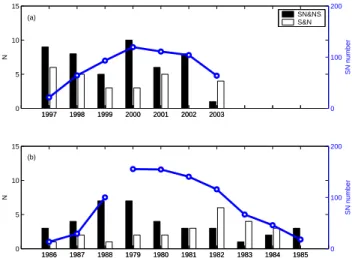
1997 1998 1999 2000 2001 2002 2003 0 5 10 N SN NS 1997 1998 1999 2000 2001 2002 2003 0 100 200 SN number 1986 1987 1988 1979 1980 1981 1982 1983 1984 1985 0 5 10 N 1986 1987 1988 1979 1980 1981 1982 1983 1984 1985 0 100 200 SN number (a) (b)

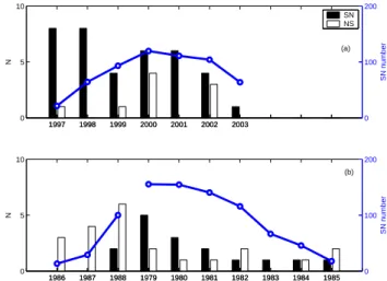
Fig. 5. Yearly number of MCs with magnetic field rotations from

the south to the north (black) and from the north to the south (white) in our study (a) and in Mulligan et al. (1998) study (b). In (b) the years have been arranged to coincide with the years of approxi-mately the same solar cycle phase in (a).

MCs were left-handed and 48% right-handed. Bothmer and Schwenn (1998) also identified an almost equal distribution: 51% left-handed and 49% right-handed MCs. In the set of MCs identified by Mulligan et al. (1998), 59% were right-handed and 41% left-right-handed. For the three and one-half year period Lynch et al. (2003) found 55% left-handed and 45% right-handed MCs.

For the handedness of an MC there is no dependence on the solar cycle phase. The equal distribution between left-and right-hleft-anded MCs is expected over a time period of sev-eral years because gensev-erally left-handed MCs originate from the Northern Hemisphere and right-handed MCs from the Southern Hemisphere, Bothmer and Schwenn (1994); Rust (1994). This is based on the agreement of the field structure of MCs with the magnetic structure of the associated fila-ment. Bothmer (2003) investigated in detail the solar sources of five MCs that are included in Table 2 (10–11 January 1997; 22 September 1997; 16–17 April 1999; 21–22 Febru-ary 2000; 15–16 July 2000). All of these five MCs followed the hemispheric rule. All front-side halo CMEs associated with these MCs originated from magnetic structures overly-ing polarity inversion lines and four of the five MCs were associated with disappearing Hα filaments.

3.3.2 SN vs. NS MCs

The distribution of bipolar (θC<45◦) MCs between those

with the magnetic field rotation from the south to the north (SN) and from the north to the south (NS) in our study (a) and in the Mulligan et al. (1998) work (b) is displayed in Fig. 5. For the first three years of the investigated period (1997–1999) all bipolar MCs, except two (16 May 1997 and 18 February 1999) had southward fields in the leading part. The number of NS-type MCs increased during the last four years of the study: In 2000 we identified four and in 2002

three NS-type MCs. The start of the change in the lead-ing polarity of MCs at solar maximum was also observed by Bothmer and Rust (1997), Bothmer and Schwenn (1998) and Mulligan et al. (1998). As seen from Fig. 5b (note the arrangement of the years) during solar maximum and the de-clining phase of solar cycle 21 (1978–1984) both SN and NS type MCs were observed. The NS type MCs clearly domi-nated the SN type MCs from solar minimum to the next solar maximum (1985–1988).

3.3.3 Bipolar vs. unipolar MCs

Figures 6 and 7 display the changes in the axial inclination of the MCs as a function of time between 1997 and 2003. Figure 6 shows the variation of the absolute value of the in-clination angle θCand Fig. 7 displays the yearly distribution

between unipolar (i.e. θC>45◦) and bipolar (θC<45◦) MCs

in our study (a) and in the Mulligan et al. (1998) work (b). MCs had a wide range of inclination angles (1◦−78◦) and the scatter in Fig. 6 is large. The evolution of |θC|in time

and the distribution of MCs between bipolar and unipolar in Fig. 7a reveal no systematic trend. We observed unipo-lar MCs frequently in the declining phase (2001 and 2003), but also during the rising activity phase (1997–1999) when each year about 40% of all identified MCs were unipolar. In 2000 and 2002 most MCs were bipolar. During the three years (1982–1984) of the late declining phase Mulligan et al. (1998) observed 13 unipolar MCs (70%) compared to only four unipolar MCs (21%) observed during the three years of the rising phase (1986–1988).

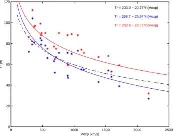
3.4 Predicted travel times of MCs to 1 AU

We studied carefully the LASCO and EIT images to find pos-sible solar causes for each MC event at 1 AU. As the earth-ward coming CMEs appear as halos in the LASCO cororon-agraph images their line-of-sight speed cannot be measured directly and arrival times to 1 AU are hard to predict. For halo CMEs the radial speed is inaccessible, but the expan-sion speed can be determined. The method to determine the expansion speed is described in dal Lago et al. (2003) and Schwenn et al. (2005). Schwenn et al. (2005) measured Vexp

for 75 LASCO CMEs which they were able to uniquely as-sociate with shock waves in the SOHO, ACE or WIND solar wind data. For each CME-shock pair, the travel time (Tr) to

1 AU was determined. The function

Tt r=203.0 − 20.77 ln(Vexp) (2)

fits the data best. In our study we found a unique CME as-sociation for 26 MCs for which we were able to measure the expansion speed. We excluded many events that had a CME association, but for which the EIT images did not show clear front side activity. Also, in some cases there were multiple CME candidates in a sufficient time window or for a single CME no unique association at 1 AU could be defined.

Figure 8 shows the travel times for MC leading edges (red stars) and for shocks (blue stars) plotted vs. the halo

ex-19970 1998 1999 2000 2001 2002 2003 2004 10 20 30 40 50 60 70 80 90 year | θC |

Fig. 6. Inclination angle θCwith respect to the ecliptic plane.

1997 1998 1999 2000 2001 2002 2003 0 5 10 15 N SN&NS S&N 1997 1998 1999 2000 2001 2002 2003 0 100 200 SN number 1986 1987 1988 1979 1980 1981 1982 1983 1984 1985 0 5 10 15 N 1986 1987 1988 1979 1980 1981 1982 1983 1984 1985 0 100 200 SN number (a) (b)

Fig. 7. Yearly number of bipolar (black) and unipolar (white) MCs

in our study (a) and in Mulligan et al. (1998) (b). In (b) the years have been arranged to coincide with the years of approximately same solar cycle phase in (a).

pansion speed. The black dashed line indicates the calcu-lated travel time from Eq. (2). A least-square fit curve of the same functional form as Eq. (2) but with newly derived co-efficients using travel times of 25 MC shocks in our study,

Tt r=236.7−25.94ln(Vexp) is indicated by the blue line. The

red line shows the same for CME-MC leading edge pairs,

Tt r=233.9−23.55ln(Vexp). The standard deviation is 11.4 h

for 26 MC leading edge pairs, and 9.66 for 25 CME-shock pairs in our study, while for the 75 CME-shocks in ? it was 14 h. The scatter in Fig. 8 is still substantial. One would expect to find an improvement when the travel time of the MC leading edge or shocks is used instead of the travel time of all the uniquely CME associated shocks at 1 AU. A shock is a larger scale structure than the CME driving it (Sheeley, 1985). When the shock-CME ejecta structure is cut at the flanks where CME material is not present, Tt r is increased

0 500 1000 1500 2000 2500 0 20 40 60 80 100 120 Vexp [km/s] Tr [h] Tr = 203.0 − 20.77*ln(Vexp) Tr = 236.7 − 25.94*ln(Vexp) Tr = 233.9 − 23.55*ln(Vexp)

Fig. 8. Travel times for shocks (blue stars) and MC leading edges

(red stars) vs. halo expansion speed. The black dashed line gives the least-squares fit for 75 CME-shock pairs in Schwenn et al. (2005). Blue and red lines give the least-squares fit for 26 CME-shock and CME-MC leading edge pairs in this study.

relative to the shock-CME structure that is cut near the cen-ter. In this study we have correlated halo CMEs to MCs. Thus, for all events the structure is cut relatively close to the center (as otherwise they would not have been identified MCs at all).

4 Geoeffectiveness of MCs

The geoeffectiveness of the identified as MCs was examined using the 1-h Dst index. Final values of Dst were available

for 1997–2002 and preliminary values were used for 2003. In the figures presented in this section we also give the pressure corrected Dst (Dst∗), where the contribution of the

magne-topause currents have been removed by using the equation in Burton et al. (1975):

D∗_st =Dst−bpPdyn+c, (3)

where Pdynis the solar wind dynamic pressure and for

con-stants b and c we have used values b=7.26 nT(nPa)1/2 and

c=11 nT derived by O’Brien and McPherron (200a). Fol-lowing the classification by Gonzalez et al. (1994) we de-fined moderate storms to have their Dst minimum between −50 nT and −100 nT and intense storms to have the Dst

min-imum <−100 nT. We have taken into consideration whether the storm was caused by southward fields embedded in the MC part itself or by sheath fields. We defined the cause of the storm as the structure (i.e. sheath or MC) during which

Dst reached 85% of its minimum for that particular storm.

Column 12 in Table 2 shows the Dst minimum (if it is less

than −50 nT) for each MC. If the sheath caused the storm, we have indicated it by “sh” and the Dst minimum follows

in parentheses. We have excluded an event (9 June 1997) that occurred in the recovery phase of the previous storm, as

the contribution of the MC fields to the Dstbehavior was not

clear. When Dst had more than one depression before

attain-ing its minimum value, we used the definition described by Kamide et al. (1998) to determine whether the event was in-terpreted as a two-step magnetic storm or two separate mag-netic storms: Assume that the magnitude of the first Dst

de-pression is A and Dst recovers by an amount C before the

second depression. If C/A>0.9, the Dst decreases are

clas-sified as two separate magnetic storms.

Gonzalez et al. (1994) presented solar wind threshold val-ues for moderate and intense storms: A moderate storm is generated when Bzis less than −5 nT for more than 2 h, and

intense storms are caused by a Bz less than −10 nT lasting

more than 3 h. Gonzalez and Tsurutani (1987) also required that in order for an intense storm to be generated the solar wind electric field (Esw) should be larger than 5 mV at least

for 3 h concurrently with Bz<−10 nT.

4.1 MCs without storms

For 21 events out of a total of 72 neither the sheath nor the MC caused the Dst decrease below our storm limit. The

majority of the 21 MCs that did not cause a storm had low magnetic field intensity or were N-type with no significant southward fields in the sheath. The average peak of the mag-netic field magnitude of all 73 MCs in our study was 18.6 nT and the average of the maximum speed inside an MC was 477 km/s (for 70 MCs, as three events lacked solar wind mea-surements). The average peak magnetic field for the 20 non-geoeffective MCs was only 13.2 nT and the average speed was slightly less than that for all MCs, 463 km/s. An exam-ple of a non-geoeffective ENW-type MC on 22 September 1997 has been presented by Bothmer (2003).

Three events from these 21 cases fulfilled the Gonzalez et al. (1994) threshold for a moderate storm: 15–16 July 1997; 3–4 August 1997 and 25 March 1999. The solar wind mea-surements from WIND and the geomagnetic response for the MC on 3–4 August 1997 are shown in Fig. 9. The figures show the magnetic field intensity, Bzcomponent (in the GSM

coordinate system), solar wind electric field, dynamic pres-sure, and the Dst index (solid line) with the pressure

cor-rection (dashed line). The data have not been shifted to the magnetopause. WIND was located at the GSE position of (X,Y ,Z)=(80, 70, 12) REand the time delay from WIND to

the magnetopause was about 20 min. The leading edge of the MC arrived at WIND at 14:00 UT on 3 August. Within the MC the magnetic field vector rotated from the south to the north. The magnetic field Z-component was less than

−10 nT (with a minimum value −13 nT) for more than 4 h, with concurrently Esw larger than 5 mV/m for about three

and one-half hours. This event even met the criteria for an intense magnetic storm, but Dst decreased only to −49 nT

4.2 Sheath storms

In 16 cases the Dst minimum of the storm was caused by

sheath fields preceding the MC. In six cases the following MC had southward fields in the leading part. The SN-type MC observed on 15–16 May 1997 had a Bzless than −10 nT

for about three and one-half hours, with the minimum value of −24 nT. This MC would have been geoeffective itself, but during the sheath Dst decreased to −100 nT, that is 87% of

the storm Dst minimum of −115 nT that was reached only

four hours later. Thus, this was classified as a sheath storm according to our definition. However, the contribution of the magnetopause currents to Dst was larger during the sheath

than during the MC, and the pressure corrected Dst reached

its minimum already during the sheath (Liemohn et al, 2001). MCs whose sheath region caused a storm had an average peak magnetic field magnitude of 16.6 nT (slightly less than the average value of all MCs). The average of the maximum speed was 519 km/s, that is above the average for all MCs. This is as expected, as the draping of the ambient interplan-etary magnetic field about the CME in the sheath is more efficient the larger the CME speed is relative to the ambient plasma (Gosling and McComas, 1987).

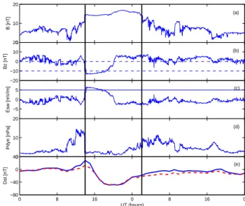
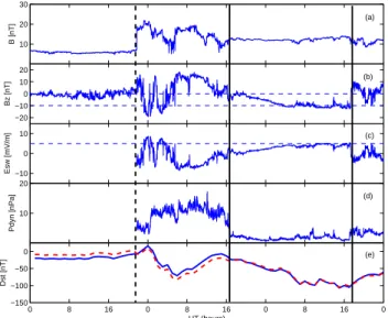
Figure 10 shows an example of an SN-type MC on 6–7 November 2000 whose sheath region caused an intense mag-netic storm. The shock was observed at ACE on 6 November at 09:08 UT. ACE is located near the L1 point ∼220 REfrom

the Earth so the time delay from ACE to the magnetopause was about 40 min. In the sheath the IMF was mainly south-ward and caused the Dstdecrease to −159 nT (D∗st−172 nT)

on 6 November at 22:00 UT. The Dst minimum was clearly

caused by the sheath fields as the front edge of the MC reached the magnetopause on 6 November at 23:00 UT. In the end of the sheath region the IMF turned northward and

Dst started to recover. A few hours later southward fields

in the leading part of the MC caused a second depression of Dst. Before the Dst minimum in the sheath Bz was less

than −10 nT for nearly four hours with the minimum value at −13 nT.

It is interesting to compare the interplanetary conditions and geomagnetic responses between the events presented in Figs. 9 and 10. The magnitude and duration of southward Bz

before the Dstminimum were comparable between these two

events. The solar wind speed was somewhat higher during the 6–7 November 2000 sheath than during the 3–4 August 1997 MC, and the maximum of the solar wind electric field were 8 mV/m and 6.5 mV/m, respectively. It seems quite peculiar why the Bz conditions shown in Fig. 10 led to an

intense magnetic storm while those presented in Fig. 9 did not cause a storm at all. During southward IMF for the 3–4 August 1997 event the dynamic pressure was low (∼2 nPa) while for the 6–7 November 2000 event the dynamic pressure was up to 15 nPa. The relative change in D_st∗ was 62 nT for the 3–4 August 1997 event and 143 nT for the 6–7 November 2000 storm. 0 10 20 B [nT] −20 −10 0 10 20 Bz [nT] −5 0 5 Esw [mV/m] 0 10 20 Pdyn [nPa] 0 8 16 0 8 16 0 −80 −40 0 40 Dst [nT] UT (hours) (a) (b) (c) (d) (e)

Fig. 9. Solar wind parameters and geomagnetic indices for a 2-day

interval from 3–4 August 1997 measured by WIND. The figures from top to bottom show magnetic field strength (a), magnetic field

Bz-component in the GSM coordinate system (b), solar wind

dy-namic pressure (c), solar wind electric field (d) and the Dst index

(solid line) together with the pressure corrected Dst (dashed line)

(e). Two solid lines indicate the interval of an MC.

10 20 30 B [nT] −20 −10 0 10 20 Bz [nT] −10 0 10 Esw [mV/m] 10 20 30 Pdyn [nPa] 0 8 16 0 8 16 0 8 16 0 −200 −100 0 Dst [nT] UT (hours) (a) (b) (c) (d) (e)

Fig. 10. Solar wind parameters and geomagnetic indices for a 3-day

interval from 6–8 November 2000 measured by ACE. The figures from top to bottom are the same as in Fig. 9. The dashed line indi-cates the shock and two solid lines indicate the interval of an MC.

4.3 Moderate and intense storms

Southward fields within the MC part itself caused 15 mod-erate storms and 20 intense storms. On the average the geo-effective MCs had a larger peak magnetic field magnitude (21.7 nT) and the speed was of the same order as the aver-age of all MCs (472 km/s). MCs on 15–16 July 2000 and 29–30 October 2003 that caused major magnetic storms and

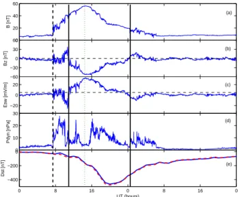
0 20 40 60 B [nT] −60 −30 0 30 60 Bz [nT] −20 0 20 Esw [mV/m] 0 10 20 30 Pdyn [nPa] 0 8 16 0 8 16 0 −400 −200 0 Dst [nT] UT (hours) (a) (b) (c) (d) (e)

Fig. 11. Solar wind parameters and geomagnetic indices for a

2-day interval from 20–21 November 2003 measured by ACE. The figures from top to bottom are the same as in Fig. 9. The dashed line indicates the shock and two solid lines indicate the interval of the MC. 0 8 16 0 8 16 0 −500 −400 −300 −200 −100 0 Dst [nT]

Fig. 12. Measured and predicted Dst development for 20–21

November 2003. The blue solid line is the 1-h Dst index and the

purple dashed line is D_st∗. The green open circles show the pre-dicted D_st∗ using the O’Brien and McPherron (2000a) model and the red stars the predicted D∗_stusing the Wang et al. (2003a) model.

had very intense magnetic fields, lacked solar wind measure-ments.

The MC on 10–11 January 1997, see Bothmer (2003), caused only a moderate storm (Dst minimum −78 nT),

al-though Bz had values less than −10 nT (with the minimum

value −15 nT) for four and one-half hours, and Esw was

larger than 5 mV/m for more than six hours. The dynamic pressure was low (2–4 nPa) during southward IMF. The 16– 17 April 1999 MC, see Bothmer (2003) and also the 16 November 1999 MC had Bz less than −10 nT longer than

3 h. During the 16–17 April 1999 event Esw was larger than

5 mV for two and one-half hours and the 16 November 1999 event lacked solar wind measurements. They both caused moderate storms (−91 nT and −79 nT).

It was shown by Huttunen and Koskinen (2004) that sheath regions were the most important drivers of intense magnetic storms during the period 1997–2002. However, three of the four most intense magnetic storms associated with the

Dst decrease below −300 nT during the solar cycle 23 were

driven primarily by southward fields in an MC. These storms were the “Bastille Day” storm on 15–16 July 2003, the first of the “Halloween storms” on 29–30 October 2003 (the sec-ond Halloween storm on 31 October 2003 was presumably driven by sheath fields) and the storm on 20–21 November 2003. This is understandable because only within MCs the southward magnetic field can obtain highest intensities. 4.3.1 20–21 November 2003 storm

Figure 11 shows an example of the intense magnetic storm on 20–21 November 2003 that was driven by southward fields in MC. When defined by Dst this was the most intense

mag-netic storm during the solar cycle 23. An interplanetary shock was observed at ACE on 20 November at 07:27 UT. In the sheath the magnetic field fluctuated from the south to the north and initiated the Dst decrease below −50 nT.

A very well-defined MC arrived at ACE on 20 November at 11:00 UT. The calculated orientation of the MC’s axis was (φC, θC)=(40◦, 71◦). The MC can be classified as the

flux-rope category ESW and the variation in the magnetic field was right-handed. The magnetic field Z-component was southward during the whole passage of the MC and the max-imum of the magnetic field coincided approximately with the minimum value of Bz. The magnetic field magnitude was

ex-ceptionally high, almost 60 nT, and the minimum value of Bz,

was −53 nT, was reached at 15:12 UT on 20 November, after which the magnetic field vector rotated slowly back to zero. Solar wind dynamic pressure was high inside the MC. South-ward MC fields caused most of the Dst decrease and the

min-imum value of Dst, −465 nT (Dst∗ −479 nT), was reached at

20:00 UT on 20 November.

Figure 12 shows the predicted D_st∗ development accord-ing to the O’Brien and McPherron (2000a) and Wang et al. (2003a) models. The O’Brien and McPherron (2000a) model assumes that the ring current injection and ring current decay parameter are controlled by the solar wind electric field. The Wang et al. (2003a) model is a modification of the O’Brien and McPherron (2000a) model and includes the influence of the solar wind dynamic pressure in the injection function and the decay parameter. Wang et al. (2003a) predicts notably well the magnitude of the D∗_st minimum while the O’Brien and McPherron (2000a) model clearly underestimates the

D∗_stminimum (the O’Brien and McPherron (2000a) model is adjusted to Dst>−150 nT). Thus, it seems that for this storm

the solar wind dynamic pressure had an important contribu-tion to the ring current development. This is also seen from Fig. 11 as Dst was further depressed by about 200 nT after

the magnetic field had turned less southward and the dynamic pressure was increased to about 20 nPa.

The MC on 20–21 November was most probably caused by a halo CME detected in LASCO images on 18 November 2003. The CME was first detected at the LASCO C2 field of view at 08:50 UT. EIT images showed activity almost at the center of the solar disk. Two M-class flares (M3.2 and M3.9) occurred in the active region 501, located almost at the center

10 20 30 B [nT] −20 −10 0 10 20 Bz [nT] −10 0 10 Esw [mV/m] 10 20 Pdyn [nPa] 0 8 16 0 8 16 0 8 16 0 −150 −100 −50 0 Dst [nT] UT (hours) (a) (b) (c) (d) (e)

Fig. 13. Solar wind parameters and geomagnetic indices for a 3-day

interval from 12–14 October 2000 measured by ACE. The figures from top to bottom are the same as in Fig. 9.

of the solar disk (N00E18) at 07:52 UT and 08:31 UT. Addi-tionally, Hαimages show a disappearance of a large filament

structure south of the active region. 4.3.2 Main phase development

Kamide et al. (1998) suggested that the two-step develop-ment of Dst that is present for more than 50% of intense

storms can be caused when southward Bzfields are present

both in the sheath and in the MC. For SN-type MCs the av-erage time difference between the Dstpeaks was small (7 h)

because of the close spatial proximity of the sheath fields and the southward Bzin the MC.

For NS-type MCs the separation between southward Bz

fields in the sheath and in the MC can be so large that Dsthas

enough time to recover to non-storm values and two separate magnetic storms follow. Figure 13 shows an NS-type MC that was observed by ACE during 13–14 October 2000. The shock arrived at ACE at 21:36 UT on 12 October. The sheath caused a moderate storm with the Dstminimum −71 nT (Dst∗ −81 nT) on 13 October, 06:00 UT. The southward Bzin the

trailing part of the MC caused an intense storm, with the

Dst minimum was −107 nT (Dst∗ −105 nT) on 14 October

15:00 UT. The time difference between the two Dst minima

was 34 h.

Another NS-type MC that caused two separate magnetic storms occurred on 28–29 July 2000. The storm caused by the sheath had the Dst minimum of −51 nT (Dst∗ −60 nT)

and 27 h later the MC caused a Dst minimum of −71 nT

(D∗_st −79 nT). From the remaining seven identified NS-type MCs, one caused an intense storm (30 September – 1 Au-gust 2002), but there was no significant southward Bzin the

sheath; four mcs were not geoeffective at all and in two cases only sheath fields caused the storm.

39% 17% 19% 25% SN (37) 33% 22% 22% 22% NS (9) 40% 60% S (15) 33% 67% N (12) no storm sheath moderate intense

Fig. 14. The effect of the flux rope type to the geoeffectivity.

Num-bers in the parentheses show the total numNum-bers of MCs identified in each category. Different colors demonstrate the different geomag-netic response: no storm at all, Dst>−50 nT (black); sheath region

generated a storm (dark gray); MC caused a moderate storm (light gray); MC caused an intense storm (white).

4.4 Geomagnetic response of MCs with different flux rope types

Figure 14 summarizes the geomagnetic response of MCs be-longing to different flux rope categories. The pie-diagrams in the top part of the figure show the distribution for bipolar MCs. In more than half of the events either the sheath region caused the storm or no significant activity at all was gener-ated. It is interesting to note that when geoeffective, the SN type MCs caused more intense storms than moderate storms. For bipolar MCs the respond depends clearly on the direc-tion of the magnetic field on the axis. In total we identified 15 S-type MCs. As seen from Fig. 14 all of them caused a storm: nine caused an intense storm (23 November 1997; 18 February 1998; 9 November 1998; 13 November 1998; 20 March 2001; 22 April 2001; 3 October 2001; 30 October 2003; 20 November 2003) and six caused a moderate storm (27 May 1999; 17 April 1999; 23 August 1999; 5 March 2001; 29 February 2002; 20 March 2003).

From 12 N-type MCs none caused a storm. However, for eight N-type MCs the sheath region preceding the MC gen-erated a storm. Half of these were intense magnetic storms. For example, the sheath preceding the N-type MC on 25–26 September 1998 caused an intense magnetic storm with the

Dst minimum −207 nT.

5 Discussion

We have investigated the properties of 73 MCs identified from WIND and ACE measurements during 1997–2003, covering rising, maximum and early declining phases of

so-lar cycle 23. The investigated period does not cover the whole solar cycle 23, but we have almost continuous cov-erage of solar wind measurements. We applied the minimum variance analysis to determine whether the preselected can-didate MC regions exhibited smooth rotation of the magnetic field in one plane. We also required that MCs must be low-beta structures (averages values of low-beta within the MC less than 0.5) with the maximum magnetic field magnitude 8 nT or larger and the duration at least 6 h.

We identified the largest number of MCs during the early rising phase when the solar activity was still low (1997– 1998). The number of observed MCs dropped in 1999, but increased again at solar maximum (2000). After that the MC rate started to decrease with the declining solar activity. The number of MCs observed at 1 AU did not correlate with the number of wide (angular width >120◦_{) LASCO CMEs.}

Cane and Richardson (2003) found that near solar minimum nearly 100% of all observed ICMEs at 1 AU had the MC structure and the fraction decreased to 10–20% when solar maximum was reached.

The occurrence rate of MCs is naturally affected by the criteria used to define an MC. In general, MCs are easier to identify from the solar wind near solar minimum than so-lar maximum. Near soso-lar maximum the mutual interaction between CMEs and the ambient solar wind can lead to com-plex structures at 1 AU where the individual characteristics of CME(s) are no longer visible, Gopalswamy et al. (2001); Burlaga et al. (2001); Wang et al. (2003b). A large fraction of MCs can be associated with disappearing filaments, Wilson and Hildner (1986); Bothmer and Schwenn (1994); Both-mer and Rust (1997) and it is likely that CMEs originating from the active regions rarely have an MC structure. Fila-ments drift towards poles when solar activity increases, con-trary to the sunspots and active regions that migrate towards the equator (Hundhausen, 1993). Near solar minimum there are few active regions and the filament disappearances occur close to the equator. Furthermore, it has been shown that near solar minimum CMEs are systematically deflected equator-ward by the fast solar wind flow originating from large polar coronal holes (Cremades and Bothmer, 2004). This suggests that most solar minimum CMEs have an MC structure and when encountering the Earth they are crossed near the axis. Near solar maximum the filament eruptions occur mainly at high latitudes and the number of CMEs are not deflected at all or are deflected towards the poles (Cremades and Both-mer, 2004). As a consequence, MCs arising from these fila-ment sites miss the Earth completely or are crossed far from the axis. The earthward-directed CMEs that mainly originate from the active regions near the equator do not generally have the MC structure. Wu et al. (2003) pointed out that the low number of MCs observed in 1999 was likely due to the fact that most filament disappearances occurred at very high lat-itudes this year. The total number of MCs that encountered the Earth during the solar maximum years was likely larger than reported in Table 2, but our criteria did not identify these as MCs. Also, it should be noted that although we could reli-ably identify all MCs at 1 AU, we could not necessarily draw

conclusions about the total number of MCs expelled from the Sun, as an increasingly larger amount of MCs are ex-pelled from higher latitudes never reaching the Earth when solar maximum is approach.

We identified somewhat more left-handed than right-handed MCs (58% and 42%). Also, in the previous studies the total amount of left-handed MCs was slightly larger than the total amount of right-handed MCs. The equal amount of left-handed and right-handed MCs is expected over the time interval of several years, as left-handed MCs originate from the Northern Hemisphere and right-handed MCs from the Southern Hemisphere, Bothmer and Schwenn (1994); Rust (1994). The largest difference was observed during the years of high solar activity (1999–2001) when the magnetic equa-tor of the Sun is not as well defined as near solar minimum.

From minimum variance analysis we obtained the esti-mation for the orientation of the MC axes that we used to separate MCs from those lying near the ecliptic plane (bipo-lar, θC<45◦) and those perpendicular to the ecliptic plane

(unipolar, θC>45◦). In total we identified 46 bipolar MCs

(63% from all MCs). During the rising phase nearly all iden-tified bipolar MCs were of the type SN. At solar maximum and in the declining phase several NS-type MCs were ob-served.

Figure 18 in Bothmer and Rust (1997) demonstrates how the magnetic structures of filaments and overlying magnetic arcades are associated with the flux rope types of MCs and their solar cycle changes. The suggested pre-eruptive con-figuration of MCs consists of large-scale magnetic field ar-cades overlying neutral lines/filament sites in bipolar regions, e.g. Gosling et al. (1995); Martin and McAllister (1997). The number of bipolar regions increases clearly when the solar activity is high and the pre-eruption field configura-tion may also form between two neighboring bipolar regions, Tandberg-Hanssen (1974); Tripathi et al. (2003). MCs origi-nating from the magnetic field configuration connecting two bipolar regions would have a different sense of rotation than those forming from a single bipolar region. Furthermore, both NS- and SN-type MCs are observed during the periods when magnetic regions from both the old and the new cycle are present, i.e. during the declining activity cycle. In the minimum and rising activity phases, when only a few bipolar regions from a single cycle are present, the majority of MCs have the same sense of magnetic field rotation.

In total, we found 23 unipolar MCs (37%). Mulligan et al. (1998) suggested that the orientation of the coronal streamer belt controls the inclination angle of the MC axis. They in-terpreted their results that unipolar MCs are most frequent in the declining phase when the neutral line is in many re-gions tilted at large angles to the solar equator, while dur-ing solar minimum and the risdur-ing phase, when the streamer belt is more equatorial, MCs are mainly bipolar (Hoeksema, 1995). This is not consistent with our study, as we frequently observed unipolar MCs in the rising phase, where the frac-tion of unipolar MCs was about 40% for each year, while at maximum and in the declining phase the fraction varied from 0 to 80%. We found no clear and systematic trend in the axial

orientation of MCs with respect to the ecliptic. Marubashi (1997) and Zhao and Hoeksema (1998) have demonstrated that the orientation of the MC axis relative to the ecliptic plane correlates rather well with the tilt of the associated fil-ament relative to the solar equator. For filfil-aments studied by Cremades and Bothmer (2004) between 1996 and 2002 no systematic trend was observed in the tilt, but a tendency for low inclined cases was observed after 2000. Apparently, the deflection of CMEs by the ambient coronal solar wind flow can deviate the CME axis from the associated filament orien-tation (Cremades and Bothmer, 2004).

The geomagnetic response of MCs was investigated using the 1-h Dst index. We focused on whether the storm was

caused by sheath fields or by the MC itself. Sheath regions are often associated with a fluctuating IMF direction and high dynamic pressure while MCs have a smoothly changing IMF direction and low dynamic pressure. Thus, they put the mag-netosphere under very different solar wind input, (Huttunen et al. (2002a); Huttunen and Koskinen (2004). About one-third of MCs that encounter the Earth do not cause a storm at all (when defined as Dst<−50 nT). These MCs are typically

somewhat slower and have lower magnetic field magnitudes than the average MC at 1 AU. We found that a sheath region caused a storm in almost one-fourth of the cases. Thus, in half of the events the southward Bzembedded in the MC was

the primary cause of the storm. MCs are inclined to cause in-tense magnetic storms since out of 35 storms caused by MCs, 20 had a Dst below −100 nT. However, six MCs that met the

solar wind threshold criteria for moderate or intense storms, Gonzalez et al. (1994), had a Dst response less intense than

expected. Tsurutani et al. (2003) investigated ring current in-tensification during 11 storm main phases in 1997 that were caused by a smoothly varying Bzcomponent within MCs. In

5 cases they found a lack of substorm expansion phase for a long period which they suggested to be the cause of the low intensity of the storm.

The geomagnetic response of an MC depends greatly on its flux-rope type. For the S-type MC the magnetic field is purely southward at the axis where the magnetic field has its maximum value, see Eq. (1). All 15 identified S-type MCs caused a storm, nine of them an intense storm (e.g. the largest storm of the solar cycle 23 on 19–20 November 2003). On the contrary, from the 12 identified N-type MCs none caused a storm, but for eight of these MCs the sheath region preced-ing the MC itself was geoeffective. There are still large un-certainties in determining the travel time of the CMEs from the Sun to the Earth (?). We investigated the relation between the travel time of the MC shock and the leading edge to 1 AU and the expansion speed of the associated halo CME. The results were slightly better in comparison to ?, who investi-gated the relationship between expansion speed and all halo CME associated shocks at 1 AU.

6 Summary

The magnetic structure and geomagnetic response of MCs detected by the WIND and ACE satellites are investigated during solar cycle 23. The results confirm the solar cycle evolution in the leading polarity of MCs found for the pre-vious cycles (21–22) by Bothmer and Rust (1997), Both-mer and Schwenn (1998) and Mulligan et al. (1998), but we did not find a clear and systematic trend in the axial inclination of MCs with respect to the ecliptic. MCs that are highly-inclined (“unipolar”) were frequently observed al-most throughout the time investigated. This result is impor-tant for the predictive purposes, as unipolar MCs that have the field southward at the axis are particularly geoeffective. In the rising phase nearly all “bipolar” MCs that are lying near the ecliptic plane were associated with the SN rotation. At solar maximum and in the declining phase the number of bipolar MCs with the opposite sense of rotation was in-creased. We suggest that at solar maximum the grouping of bipolar regions and in the declining phase the presence of magnetic regions from both new and old solar cycles, results in the mixture of NS and SN type MCs.

The geomagnetic response of MCs varied greatly depend-ing on the inferred flux-rope category. When geoeffective, the MCs have a tendency to cause intense magnetic storms. By distinguishing the contribution of the sheath region and the MC itself we find that in the considerable fraction of cases (22%) the sheath region caused the Dstminimum of the

storm. In particular, the intensity and duration of southward

Bz in the sheath is crucial for N-type MCs, as they are not

geoeffective themselves. In principle, the flux-rope type of an MC can be deduced in advance from the magnetic struc-ture of the associated filament, e.g. Bothmer and Schwenn (1998), but for the sheath fields no practical method has been developed. Another important aspect is to reliably predict the time of the storm. As shown in this study, there are still large uncertainties in determining the MC arrival time from the Sun to 1 AU. Whether the storm is caused by the south-ward Bzvalues in the sheath, in the leading part of the MC or

in the trailing part of the MC, can make a large difference as to the timing of the storm. Particularly, an NS-type MC may cause two separate magnetic storms due to a long separation of southward fields in the sheath and in the MC between.

Acknowledgements. We thank R. Lepping for the WIND magnetic

field data, and K. W. Ogilvie for the WIND solar wind data. We also thank N. Ness for the ACE magnetic field data and, D. J. McComas for the ACE solar wind data. These data were obtained through Coordinated Data Analysis Web (CDAWeb). The LASCO CME catalog is generated and maintained by NASA and The Catholic University of America in cooperation with the Naval Research Lab-oratory. SOHO is a project of international cooperation between ESA and NASA. The yearly sunspot numbers were obtained from RWC Belgium World Data Center for the Sunspot Index. The Dst

and Kp values were obtained from the World Data Center C2 in

Kyoto. The study was supported through the Antares programme of the Academy of Finland.

Topical Editor R. Forsyth thanks C. Cid and another referee for their help in evaluating this paper.