HAL Id: hal-00317168
https://hal.archives-ouvertes.fr/hal-00317168
Submitted on 1 Jan 2003
HAL is a multi-disciplinary open access
archive for the deposit and dissemination of
sci-entific research documents, whether they are
pub-lished or not. The documents may come from
teaching and research institutions in France or
abroad, or from public or private research centers.
L’archive ouverte pluridisciplinaire HAL, est
destinée au dépôt et à la diffusion de documents
scientifiques de niveau recherche, publiés ou non,
émanant des établissements d’enseignement et de
recherche français ou étrangers, des laboratoires
publics ou privés.
Measurement of the stochasticity of low-latitude
geomagnetic temporal variations
J. A. Wanliss, M. A. Reynolds
To cite this version:
J. A. Wanliss, M. A. Reynolds. Measurement of the stochasticity of low-latitude geomagnetic temporal
variations. Annales Geophysicae, European Geosciences Union, 2003, 21 (9), pp.2025-2030.
�hal-00317168�
Annales
Geophysicae
Measurement of the stochasticity of low-latitude geomagnetic
temporal variations
J. A. Wanliss and M. A. Reynolds
Department of Physical Sciences, Embry-Riddle Aeronautical University, 600 S. Clyde Morris Blvd., Daytona Beach, FL 32114, USA
Received: 31 October 2002 – Revised: 24 April 2003 – Accepted: 26 April 2003
Abstract. Ground magnetometer measurements of total magnetic field strength from 6 stations at low latitudes were analyzed using power spectrum and Hurst range scaling tech-niques. The Hurst exponents for most of these time-series were near 0.5, which indicates stochasticity, with the highest latitude stations exhibiting some persistence with Hurst ex-ponents greater than 0.6. Although no definite correlations are evident, the relative increase of the Hurst exponent with latitude suggests the possibility that the underlying dynamics of the magnetosphere change with latitude. This result may help quantify the dynamics of the inner magnetosphere itself without the direct presence of the solar wind driver.
Key words. Magnetospheric physics (magnetospheric
con-figuration and dynamics; plasmasphere) – Space plasma physics (nonlinear Phenomena)
1 Introduction
Strong nonlinear coupling between the solar wind and the earth’s magnetosphere results in many dramatic disturbances in the near-earth space environment, such as the dynamic magnetic and auroral signatures as well as magnetotail plasma signatures associated with magnetic storms and mag-netospheric substorms. The strongest coupling between the solar wind and the magnetosphere occurs near the magne-topause, close to magnetic field lines that map to the high latitude ionosphere. The irregular nature of high-latitude disturbances, which typically occur above 60◦geomagnetic latitude, are clearly manifested in the auroral electrojet in-dices AE and AL. Studies of these inin-dices have suggested that the magnetosphere behaves as a self-organized system with a small number of degrees of freedom (Vassiliadis et al., 1990; Sharma et al., 1993) although there are questions as to whether the magnetosphere itself is a self-organized system or whether it simply reflects the self-organized state of the solar wind and interplanetary magnetic field (IMF) to which it is strongly coupled (Price and Newman, 2001). Correspondence to: J. A. Wanliss ([email protected])
If the magnetosphere is self-organized, it would imply that only a small number of coupled, nonlinear ordinary differen-tial equations are required to describe its dynamic behaviour. Indeed, the number of degrees of freedom that describe the high-latitude phenomena was found to have an average value of about 3.3 (Vassiliadis et al., 1990; Roberts, 1991; Shan et al., 1991; Sharma et al., 1993), although these results have been challenged by other studies (Prichard and Price, 1992, 1993). Such nonlinear approaches have led to the develop-ment and improvedevelop-ment of various dynamic models of sub-storms (Ohtani et al., 1995; Baker et al., 1997, 2000; Takalo et al., 1999; Horton et al., 2001)
Whereas the studies cited above have focused primarily on magnetic variations due to high-latitude current systems, in this paper we consider low-latitude magnetic variations (3 ∼ 35◦−40◦). The high-latitude magnetic field lines are connected to magnetospheric regions that map very closely to the solar wind but the low-latitude magnetic field lines are connected directly to the inner magnetosphere. Since the field lines at low latitudes (L ∼ 1.5 − 1.8) are almost dipo-lar, they are not as strongly influenced by the interplanetary medium as the high-latitude regions where chaotic signatures might simply reflect similar solar wind conditions. Thus, ex-amination of low-latitude ground magnetometer signals can provide clues as to whether the magnetosphere is inherently self-organized.
At lower latitudes, the dominant magnetic variations are due to the two diurnal solar quiet (Sq) large-scale current systems with foci at about 30◦magnetic latitude in the
iono-sphere and peak current densities near local noon. Super-imposed on these diurnal signals are higher frequency vari-ations from magnetospheric sources. Coupling of the low-latitude regions with the magnetosphere is achieved along magnetic field lines that map to the inner magnetosphere, and through the variation of the ring current at distances of about 3–5 earth radii (RE), especially during magnetic storms. The
references quoted above have demonstrated a clear nonlinear behaviour of high-latitude time-series, but the latitudinal ex-tent and variability of such behaviour is unknown. We are, therefore, interested in determining whether the quantitative
2026 J. A. Wanliss and M. A. Reynolds: Measurement of the stochasticity
Table 1. Geographic latitude and longitude, corrected geomagnetic
latitude, and L-shell location for the various stations Station Latitude Longitude Magnetic L
(◦South) (◦East) Latitude Ellis 23.79 27.72 −34.37 1.47 Bronk 25.62 29.05 −35.93 1.53 Lans 25.94 27.93 −36.21 1.54 Vry 27.23 24.62 −37.23 1.58 Bos 28.40 25.54 −38.18 1.62 Herm 34.42 19.27 −42.30 1.83
nonlinear dynamics of the high-latitude regions extends to lower latitudes; for example, to determine the fractal dimen-sion pertinent to low-latitudes and whether this is similar to that found in the high-latitude studies. This paper represents a preliminary effort to address the issue.
A global index that characterizes the low-latitude mag-netic variation, is Dst. However, since Dst is computed only
at hourly intervals, it was deemed advantageous to use ac-tual magnetometer records that provide a higher time res-olution in order to investigate the fractal properties present at low-latitudes. Furthermore, the individual magnetometer time-series give localized estimates of the fractal parameters rather than the global output that is sampled by geomagnetic indices. We have analyzed individual magnetometer records for five days in January 1993 during which magnetospheric activity indicates no magnetic storms although several small substorms are observed at high-latitudes. We find evidence that the dynamics of low-latitude regions of the magneto-sphere, sampled by the magnetometer stations in the study, are primarily stochastic, although two stations exhibit sig-nals that are not inconsistent with self-organized criticality but with a lower level of complexity than for the dynamics governing high-latitudes; that is, the calculated fractal di-mension is lower than that found in the high-latitude stud-ies cited above. Although the degree of coupling with the solar wind and the IMF is not clear, our results do suggest that the low-latitude inner magnetosphere behaves in a fun-damentally different way to the high-latitude regions.
2 Data
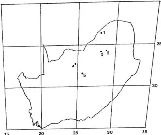
We utilize data from an Anglo American Corporation experi-ment, which recorded geomagnetic temporal variations from an array of six magnetometer stations spread in latitude over South Africa (Wanliss, 1995), shown in Fig. 1. The stations were at Ellisras (Ellis), Bronkhorstspruit (Bronk), Lanseria (Lans), Vryburg (Vry), Boshof (Bos) and Hermanus (Herm), whose geographic locations, corrected geomagnetic latitudes and L-shell positions are listed in Table 1. The motivation for the experiment was to provide a rigorous understanding of the background magnetic field in the region, to be used in the interpretation of aeromagnetic surveys. A useful
byprod-Fig. 1. Map of South Africa, showing the location of the six
magne-tometer stations used in the present study. From north to south (low latitude to high latitude): (1) Ellis, (2) Bronk, (3) Lans, (4) Vry, (5) Bos and (6) Herm. The coordinates shown are geographic.
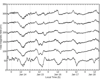
uct was the high time resolution data used in the present study. Simultaneous data from the stations were acquired during 13–18 January 1993. The magnetometer instrument sensitivity is 0.1 nT with a sampling interval of 10 s. The to-tal ambient field in the region of these low-latitude stations is approximately 30 000 nT. Figure 2 shows the time-series from each of the stations, with their mean values removed. The most obvious signatures are the diurnal Sq variations that result in minima near local noon; these exist at all sta-tions but are clearest at Hermanus, primarily due to the so-called “coastal effect” which arises due to the magnetic field induced by time varying magnetic fields in the conducting ocean water (Pal’shin et al., 1999).
The Dst index over this period indicates slowly varying
fields and no magnetic storms although several substorms were observed in the auroral signatures of the CANOPUS photometers and magnetometers. Since Dst is computed by
the convolution of magnetometer signals from stations at lat-itudes lower than about 36◦(L < 1.53) it gives a good indi-cation of the state of the inner magnetosphere at the latitudes we are examining. The mean and maximum values of Dst
during this period investigated were −15 nT and −43 nT, re-spectively, which represent a relatively small ring current en-ergy density.
3 Analysis
Since temporal variations of the geomagnetic field exhibit scale-independent behaviour, it is appropriate to analyze them with fractal methods. In the following, we examine the behaviour of the low-latitude magnetic field time-series from several different perspectives in order to determine their frac-tal characteristics. Since it is demonstrably difficult to mea-sure the chaotic variability of such space physics data, we
Table 2. For each station, the columns list the autocorrelation time, τc; the power spectral exponent, β; the corresponding Hurst exponent,
Hβ, calculated from β = 2Hβ+1; the Hurst exponent, HR/S, calculated by the R/S method; and the fractal dimension, DR/S, calculated
from DR/S = 2 − HR/S. The error listed is that from the least-squares regression and so it is only a minimum error as there are other
possible sources of error that are difficult to calculate. (The error of DR/Sis the same as that for HR/S
Station τc(hours) β Hβ HR/S DR/S Ellis 6.36 2.093 ± 0.020 0.547 ± 0.010 0.504 ± 0.017 1.496 Bronk 6.90 2.175 ± 0.013 0.588 ± 0.007 0.501 ± 0.015 1.499 Lans 5.97 1.963 ± 0.037 0.482 ± 0.019 0.492 ± 0.039 1.508 Vry 5.17 2.129 ± 0.016 0.565 ± 0.008 0.523 ± 0.016 1.477 Bos 4.71 2.328 ± 0.033 0.664 ± 0.017 0.696 ± 0.021 1.304 Herm 3.73 2.382 ± 0.014 0.691 ± 0.007 0.675 ± 0.020 1.325 0 12 0 12 0 12 0 12 0 12 0 50 100 150 200 250 300 350
Jan 14 Jan 15 Jan 16 Jan 17 Jan 18 Local Time (h)
Total magnetic field (nT)
Fig. 2. Total relative magnetic field measured at the six stations
from 13–18 January 1993. The series are plotted as a function of local time (LT) and range from top to bottom in increasing latitude. From top to bottom (1) Ellis, (2) Bronk, (3) Lans, (4) Vry, (5) Bos and (6) Herm.
have not relied on a single technique but have investigated these properties using two different methods described in the following section, viz. (1) power spectral analysis and (2) range scaling analysis (Hurst, 1951).
A third, more common, method of discerning nonlinear behaviour from a time-series is the use of embedding dimen-sion analysis to evaluate the correlation dimendimen-sion ν (Grass-berger and Procaccia, 1983). The value of ν is determined by counting the number of pairs of points in the time-series that are separated by less than the distance r. This “correla-tion integral” should scale as rν for small r. There are two major difficulties with the application of this method. First, the pairs of points must be no nearer than the autocorrela-tion time τc (e.g. Hilborn, 1994). For the time-series in this
study, τcranges from about 4–7 h (these are listed in Table 2)
which is a significant fraction of the total length of each time-series. Even when this restriction is lifted by using only dis-tant points, the strong periodic modulation due to Sq can lead
10−4 10−3 10−2 100 102 104 106 108 Frequency (Hz) Power (nT 2 /Hz) Ellis, β=2.093 ± 0.020
Fig. 3. Power spectra of magnetic data measured during 13–18
Jan-uary 1993 at Ellisras (Ellis). The best-fit line gives a value for the spectral exponent of β = 2.093 ± 0.020. This line (dashed) is shifted for the purposes of comparison.
to anomalously large ν (Shan et al., 1991). In the present case, we obtained values for ν ∼ 5 which do not agree with the more robust methods shown below, presumably due to the large correlation times as well as the Sq modulation at 24 h. This is consistent with previous results which indicate that correlation dimensions are adversely affected by strong periodic modulations (Shan et al., 1991), and when the cor-relation time is large (Shan et al., 1991; Prichard and Price, 1992).
3.1 Power spectrum analysis
A great deal of space physics data is self-affine (Ohtani et al., 1995; Takalo et al., 1999) with a power spectral density of the form P (f ) ∝ f−β, where β is the spectral exponent. The power spectrum of the time-series from the Ellis station is shown in Fig. 3 and the best-fit line (calculated over three or-ders of magnitude in frequency) indicates a spectral exponent of β = 2.093 ± 02.020. All six stations have power spectra
2028 J. A. Wanliss and M. A. Reynolds: Measurement of the stochasticity 3 4 5 6 7 8 9 10 11 0 1 2 3 4 5 6 log(n) log(R/S) Ellis, H=0.504 ± 0.017
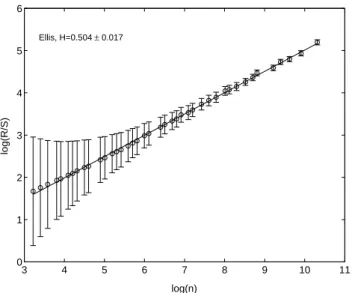
Fig. 4. Range scaling parameter (R/S) versus number of
obser-vations for the Ellis station. The best-fit line (dashed) results in a Hurst exponent of HR/S=0.504 ± 0.017.
whose exponents remain constant over a similar range of fre-quencies. The spectral exponents for all stations are listed in Table 2. With the exception of the Lanseria station, β is slightly larger than 2. This is significant because a value of β =2 corresponds to a random walk and, as investigated be-low in Sect. 3.2, a larger value indicates some “persistence” in the time-series (Mandelbrot, 1983).
It appears that β tends to increase with increasing geomag-netic latitude. A linear least-squares fit gives β = (0.95 ± 0.39)L+(0.66±0.63) which indicates a correlation between β and L. The correlation coefficient, however, is r = 0.77 which implies only a weak linear correlation. We are, there-fore, unsure of the significance of this result but find that it suggests the possibility that there is some latitudinal depen-dence in the nonlinear statistics. In addition, the autocorrela-tion time tends to decrease with increasing geomagnetic lati-tude. A best-fit line gives τc=(−8.3 ± 2.1)L + (18.7 ± 3.3)
(correlation coefficient r = −0.90). Unfortunately, these six stations have only a narrow spread in L, which means that the strength of these trends is only hinted at with the present data. In fact, we cannot say with certainty that either of these correlations is linear. However, these results do suggest the need for a study over a wider range of low-latitude L-shells which could, quantitatively, discern a trend and perhaps the physical processes of the underlying dynamics with geomag-netic latitude.
3.2 Range scaling analysis
Range scaling (R/S) analysis was developed by Hurst (1951) to study time-series whose underlying processes are inde-pendent, though not necessarily Gaussian. Here, our time-series consists of a sequence of measurements of the total magnetic field B(t0), B(t1), . . . B(tM), where t0 = 0, t1 =
τ, . . . , tM = Mτ. The time-series is characterized by an
exponent, H , which is a quantitative measure of the self-affinity of the time-series. That is, H relates the typical change in B, 1B, to the difference in time 1t by the scal-ing law 1B ∼ 1tH (Mandelbrot, 1983) where H is in the range 0 ≤ H ≤ 1. This is a nonuniform scaling where the shape of the time-series is invariant under a transforma-tion that scales the coordinates differently and is a hallmark of self-affinity. For the usual Brownian motion, which is a stochastic random walk, H = 0.5. Larger values of H in-dicate some memory or persistence. Smaller values inin-dicate “anti-persistence,” which means that the time-series is more volatile and choppy. One method of determining H is to use R/S analysis. For example, R/S analysis was recently ap-plied to the high-latitude AE index and shown to provide a robust estimator of deterministic chaos (Price and Newman, 2001).
Our analysis consisted of taking the raw positive definite time-series x(t ) of length M and taking the first differences of the natural logarithm, thus creating a new time-series B(t ). B(tp) =ln(x(tp+1)) −ln(x(tp)); p =1, 2 . . . , M − 1 (1)
Following this we take the time-series B(t ) and subtract the sample mean B to obtain a new series
Zr =B(tr) − B; r =1, 2 . . . , n (2)
Next, a cumulative time-series, Y , is derived Yl =
l
X
i=1
Zi; l =2, 3, . . . , n (3)
and an adjusted range, R, is formed in terms of the maxi-mum minus minimaxi-mum value of the cumulative series Y , R = sup(Y1, Y2, . . . , YT) − inf(Y1, Y2, . . . , YT). The rescaled
range, R/S, is then given by the ratio R/σ , where σ is the usual standard deviation. This quantity scales, with respect to T , by the power law
(R/S)T ∝TH (4)
where T = tn, and H is the Hurst exponent. The value of
H can then be evaluated from a plot of log(R/S) versus log(T ) and a measurement of the slope of the best fit line. Figure 4 shows the rescaled range R/S for the Ellis station, and a best-fit line is shown, resulting in a Hurst exponent of HR/S = 0.504 ± 0.017. The rescaled ranges for the other
stations result in similarly good linear fits. The Hurst ex-ponents, HR/S, for all the stations as calculated by the R/S
analysis are listed in Table 2.
The uncertainties in the calculated values for the Hurst ex-ponent were calculated by starting with the uncertainty in the measured magnetic field, ± 0.1 nT. These errors were propa-gated through the calculations listed above to obtain the error value for R/S (see Fig. 4). The best-fit slope in Fig. 4 was obtained through linear least-squares analysis taking into ac-count the error in the dependent variable (e.g. Press et al., 1988). All of the linear fits were consistent with the data with chi-square probabilities greater than 0.99, that is, the linear slopes are highly significant.
1.9 2 2.1 2.2 2.3 2.4 2.5 0.45 0.5 0.55 0.6 0.65 0.7 β HR/S
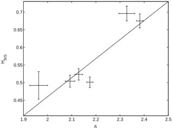
Fig. 5. Plot of HR/S(from range scaling analysis) versus β (from
power spectral analysis). The best-fit linear curve is indicated as the solid line. The straight line represents HR/S =(0.54 ± 0.13)β −
(0.62 ± 0.29).
There is no reason to expect, a priori, that there should be a linear relationship between β and HR/S. However, for
self-affine data, there is a relation between the Hurst expo-nent and the spectral expoexpo-nent, β = 2H + 1 (Turcotte, 1992, p. 78). In Table 2, therefore, the Hurst exponents as cal-culated from the measured spectral exponent (Hβ) are also
listed. Although the power spectrum and R/S analysis are independent modes of investigation, these two techniques of calculating the Hurst exponent are relatively consistent al-though they do not always agree within the estimated errors. We do not expect a perfect correspondence since the methods of investigation are independent and the calculation of R/S is significantly more stable against sudden phase changes of fluctuations than the calculation of a power spectrum. A more rigorous method to measure the strength of their agree-ment is to determine if the spectral exponent, β, is correlated to the Hurst exponent, HR/S. A linear least-squares fit results
in the relation HR/S=(0.54 ± 0.13)β − (0.62 ± 0.29) with
a correlation coefficient of r = 0.90. This result leads to the conclusion that these magnetic field time-series are self-affine (see Fig. 5). In addition, this is evidence that the data behave in a self-organized manner and the calculation of the fractal dimension is meaningful. For a time-series that can be modeled as fractional Brownian motion (Mandelbrot, 1983), the relationship between H and the fractal dimension D is
H =2 − D (5)
Under these assumptions the fractal dimensions of all sta-tions, as calculated from HR/S and Eq. (5), are listed in
Ta-ble 2. As expected, the fractal dimensions are all near 1.5 although the stations at the higher latitudes exhibit a some-what lower value for D; this is consistent with the fact that the Hurst exponents exhibit somewhat more persistence.
Similar to the autocorrelation times and spectral expo-nents, the Hurst exponent exhibits a weak correlation with
magnetic latitude or L-shell. The four lower latitude stations are consistent with H ∼ 0.5, indicating stochastic behaviour. On the other hand, the Bos and Herm stations, located at the highest L-values, demonstrate persistent behaviour (as indicated by a value of H > 0.5) which means that these time-series have long memory effects. In the language of nonlinear dynamics, the data exhibit a sensitive dependence on initial conditions, one of the hallmarks of chaos. This feature, the latitudinal dependence of nonlinear features in magnetic time-series, is strong enough to warrant further re-search. Analysis of data from other magnetometer chains (IMAGE, CANOPUS, MEASURE) is underway.
3.3 Possible systematic errors and sources of bias
Because we have used relatively short time-series, it is a rea-sonable concern that our estimates of the Hurst exponent are affected by the length of the time-series rather than by ac-tual dynamics; a time-series that is too short may bias the estimates. We have investigated this possibility by randomly reorganizing the data so that the order of observations is com-pletely different from that of the original time-series. Be-cause the actual observations remain the same, the frequency distribution of the time-series remains unchanged. If there was a long memory effect in place, the order of the data would be very important and the scrambling effect would be to destroy the structure of the system, thus resulting in a much lower Hurst exponent estimate. However, if the length of the time-series is resulting in bias, scrambling can have the opposite effect, resulting in a Hurst exponent that is even larger than the original estimate (Peters, 1991, p. 75). For stations 5 and 6 which showed persistence, we found that scrambling the original series caused a drop in the value of the Hurst exponents which shows that the long memory pro-cess was destroyed by the scrambling propro-cess. The other four stations, of course, were already stochastic and the reorder-ing process left their Hurst exponents effectively unchanged. Another reasonable concern is the affect of the periodic Sq variations which might increase the value of the Hurst expo-nent in an unphysical manner. We investigated whether this had an effect on our analysis by considering the data from the Hermanus station for the whole of January 1993 (unfortu-nately, the other stations were only temporarily in operation for the 5 days reported here). Range scaling analysis was performed on a new time-series obtained by subtracting the mean of the three quietest days of the month (21, 22, 23 Jan-uary) from the original time-series (this essentially removes the Sq effect). There was no significant change in the Hurst exponent. We further investigated this possible effect on an artificial (chaotic) time-series for the Lorenz attractor. The Hurst exponent was calculated for this time-series, and then compared to the Hurst exponent that was computed when the time-series was added to a sinusoidal curve that had 5 periods for the entire length of the series. The two Hurst exponents were statistically equal (i.e. within the error bars).
2030 J. A. Wanliss and M. A. Reynolds: Measurement of the stochasticity
4 Discussion and conclusion
Several previous studies have investigated the fractal proper-ties of high-latitude geomagnetic variations through the use of the AE and AL indices. The number of degrees of free-dom that describes the system, as measured by the correla-tion dimension, was found to be between 2.2 and 4.2 (Vassil-iadis et al., 1990; Roberts, 1991; Shan et al., 1991; Sharma et al., 1993). In the present paper, low-latitude geomagnetic variations have been examined using different fractal tech-niques that are not subject to difficulties due to long corre-lation times and strong periodicities. As stated above, indi-vidual magnetometer measurements were used because they have higher spatial and temporal resolution than a global in-dex such as Dst.
The L-shells of the stations ranged over L = 1.47 − 1.83, indicating that the stations are sampling a very different re-gion of the magnetosphere, namely the plasmasphere, to the high-latitude stations used to compute AE and AL. The pe-riod studied encompassed low dynamic magnetospheric ac-tivity, as indicated by relatively steady Dst values. This
im-plies that the influence of the ring current perturbations is not large and that the perturbations are primarily due to the ionospheric solar quiet and auroral electrojet currents, as well as possible plasmaspheric influences. The previous studies mentioned have argued that the dynamical processes associ-ated with substorms and, in particular with the AE and AL indices, are low dimensional. Here, we conclude that an even lower dimensional behavior characterizes the low-latitude magnetosphere. The average fractal dimension obtained was near D ∼ 1.5 which is lower than the high-latitude results. This might indicate that the inherent dynamical properties of the low-latitude magnetosphere are less complex and can be described by fewer degrees of freedom than the high-latitude magnetosphere that was previously examined via global in-dices. Qualitatively, the good agreement between the spectral exponent and the Hurst exponent HR/Slends credence to the
existence of self-organized behaviour at low latitudes. Perhaps the most interesting result is the correlation of ev-ery statistical property of the magnetic field time-series with magnetic L-shell. In particular, the increase of HR/S(to
val-ues greater than 0.5) with increasing L suggests that the com-plexity of the inner magnetosphere increases with magnetic latitude and L-shell. However, it is impossible to be certain of the significance of these results since we have only a small sample of data (only six stations over a very narrow latitudi-nal range). A more detailed global study, with many lati-tudinally spread stations, is necessary to determine whether the behaviour found here is consistent with that at higher lat-itudes. Of course these trends, if extrapolated to high lati-tudes, would lead to unreasonable values in the auroral re-gion. For this reason, we conclude not that the complexity increases linearly with L but only that the trend is suggested and further study is needed.
Acknowledgement. Topical Editor T. Pulkkinen thanks C. P. Price
for his help in evaluating this paper.
References
Baker, D. N., Klimas, A. J., Vassiliadis, D., Pulkkinen, T. I., and McPherron, R. L.: Re-examination of driven and unloading as-pects of magnetospheric substorms, J. Geophys. Res., 102, 7, 169–177, 1997.
Baker, D. N., Vassiliadis, D., Klimas, A. J., and Valdivia, J. A.: The nonlinear dynamics of space weather, Adv. Space Res., 26, 197–207, 2000.
Grassberger, P. and Procaccia, I.: Characterization of strange attrac-tors, Phys. Rev. Lett., 50, 346–349, 1983.
Hilborn, R. C.: Chaos and nonlinear dynamics, Oxford University Press, Oxford, 1994.
Horton, W., Weigel, R. S., and Sprott, J. C.: Chaos and the lim-its of predictability for the solar-wind-driven magnetosphere-ionosphere system, Phys. Plasmas, 8, 2946–2952, 2001. Hurst, H. E.: The long term storage capacity of reservoirs, Trans.
Am. Soc. Civil. Eng., 116, 770–799, 1951.
Mandelbrot, B. B.: The fractal geometry of nature, W. H. Freeman, New York, 1983.
Ohtani, S., Higuchi, T., Lui, A. T. Y., and Takahashi, K.: Magnetic fluctuations associated with tail current disruption: Fractal anal-ysis, J. Geophys. Res., 100, 19 135–19 145, 1995.
Pal’shin, N. A., Vanyan, L. L., Porai-Koshits, A. M., Khan, Yu. V., Kaikkonen, P., Tiikkainen, J., Matyushenko, V. A., and Lukin, L. R.: On-land measurements of the motionally-induced electric field, Oceanology, 39, 422–431, 1999.
Peters, E. E.: Chaos and order in the capital markets: the new view of cycles, prices, and market volatility, John Wiley and Sons, 1991.
Press, W. H., Flannery, B. P., Teukolsky, S. A., and Vetterling, W. T.: Numerical Recipes: The Art of Scientific Computing, Cam-bridge, 1988.
Prichard, D. and Price, C. P.: Spurious dimension estimates from time-series of geomagnetic indices, Geophys. Res. Lett., 19, 1623–1626, 1992.
Prichard, D. and Price, C. P.: Is the AE index the result of nonlinear dynamics?, Geophys. Res. Lett., 20, 2817–2820, 1993.
Price, C. P. and Newman, D. E.: Using the R/S statistic to analyze
AEdata, J. Atmos. Solar-Terr. Phys., 63, 1387–1397, 2001. Roberts, D. A.: Is there a strange attractor in the magnetosphere: J.
Geophys. Res., 96, 16 031–16 046, 1991.
Shan, L., Hansen, P., Goertz, C. K., and Smith, R. A.: Chaotic appearance of the AE index, Geophys. Res. Lett., 18, 147–151, 1991.
Sharma, A. S., Vassiliadis, D., and Papadopoulos, K.: Reconstruc-tion of low-dimensional magnetospheric dynamics by singular spectrum analysis, Geophys. Res. Lett., 20, 335–338, 1993. Takalo, J., Timonen, J., Klimas, A., Valdivia, J., and Vassiliadis, D.:
Nonlinear energy dissipation in a cellular automaton magnetotail field model, Geophys. Res. Lett., 26, 1813–1816, 1999. Turcotte, D.: Fractals and chaos in geology and geophysics:
Cam-bridge University Press, CamCam-bridge, 1992.
Vassiliadis, D., Sharma, A. S., Eastman, T. E., and Papadopoulos, K.: Low dimensional chaos in magnetospheric activity from AE time-series, Geophys. Res. Lett., 17, 1841–1844, 1990. Wanliss, J. A.: A study of temporal variations of the geomagnetic
field with reference to aeromagnetic surveys, M.Sc dissertation, Univ. of the Witwatersrand, Johannesburg, 1995.