HAL Id: hal-03174107
https://hal.archives-ouvertes.fr/hal-03174107
Submitted on 18 Mar 2021
HAL is a multi-disciplinary open access
archive for the deposit and dissemination of
sci-entific research documents, whether they are
pub-lished or not. The documents may come from
teaching and research institutions in France or
abroad, or from public or private research centers.
L’archive ouverte pluridisciplinaire HAL, est
destinée au dépôt et à la diffusion de documents
scientifiques de niveau recherche, publiés ou non,
émanant des établissements d’enseignement et de
recherche français ou étrangers, des laboratoires
publics ou privés.
stellar object candidates from IR surveys
D. Cornu, J. Montillaud
To cite this version:
D. Cornu, J. Montillaud. A neural network-based methodology to select young stellar object
can-didates from IR surveys. Astronomy and Astrophysics - A&A, EDP Sciences, 2021, 647, pp.A116.
�10.1051/0004-6361/202038516�. �hal-03174107�
https://doi.org/10.1051/0004-6361/202038516
c
D. Cornu and J. Montillaud 2021
&
Astrophysics
A neural network-based methodology to select young stellar object
candidates from IR surveys
?
D. Cornu
1,2and J. Montillaud
11 Institut UTINAM – UMR 6213 – CNRS – Univ. Bourgogne Franche Comté, OSU THETA, 41bis avenue de l’Observatoire, 25000 Besançon, France
e-mail: [email protected]
2 Sorbonne Université, Observatoire de Paris, PSL Research University, CNRS, LERMA, 75014 Paris, France Received 27 May 2020 / Accepted 5 December 2020
ABSTRACT
Context.Observed young stellar objects (YSOs) are used to study star formation and characterize star-forming regions. For this
pur-pose, YSO candidate catalogs are compiled from various surveys, especially in the infrared (IR), and simple selection schemes in color-magnitude diagrams (CMDs) are often used to identify and classify YSOs.
Aims.We propose a methodology for YSO classification through machine learning (ML) using Spitzer IR data. We detail our approach
in order to ensure reproducibility and provide an in-depth example on how to efficiently apply ML to an astrophysical classification.
Methods.We used feedforward artificial neural networks (ANNs) that use the four IRAC bands (3.6, 4.5, 5.8, and 8 µm) and the
24 µm MIPS band from Spitzer to classify point source objects into CI and CII YSO candidates or as contaminants. We focused on nearby (.1 kpc) star-forming regions including Orion and NGC 2264, and assessed the generalization capacity of our network from one region to another.
Results.We found that ANNs can be efficiently applied to YSO classification with a contained number of neurons (∼25). Knowledge
gathered on one star-forming region has shown to be partly efficient for prediction in new regions. The best generalization capacity was achieved using a combination of several star-forming regions to train the network. Carefully rebalancing the training proportions was necessary to achieve good results. We observed that the predicted YSOs are mainly contaminated by under-constrained rare subclasses like Shocks and polycyclic aromatic hydrocarbons (PAHs), or by the vastly dominant other kinds of stars (mostly on the main sequence). We achieved above 90% and 97% recovery rate for CI and CII YSOs, respectively, with a precision above 80% and 90% for our most general results. We took advantage of the great flexibility of ANNs to define, for each object, an effective member-ship probability to each output class. Using a threshold in this probability was found to efficiently improve the classification results at a reasonable cost of object exclusion. With this additional selection, we reached 90% and 97% precision on CI and CII YSOs, respectively, for more than half of them. Our catalog of YSO candidates in Orion (365 CI, 2381 CII) and NGC 2264 (101 CI, 469 CII) predicted by our final ANN, along with the class membership probability for each object, is publicly available at the CDS.
Conclusions.Compared to usual CMD selection schemes, ANNs provide a possibility to quantitatively study the properties and
qual-ity of the classification. Although some further improvement may be achieved by using more powerful ML methods, we established that the result quality depends mostly on the training set construction. Improvements in YSO identification with IR surveys using ML would require larger and more reliable training catalogs, either by taking advantage of current and future surveys from various facilities like VLA, ALMA, or Chandra, or by synthesizing such catalogs from simulations.
Key words. methods: statistical – methods: numerical – stars: protostars – stars: pre-main sequence – catalogs
1. Introduction
Observing young stellar objects (YSOs) in stellar clusters is a common strategy to characterize star-forming regions. Their presence attests star formation activity, their spatial distribution within a molecular complex provides clues about its star for-mation history (Gutermuth et al. 2011), and their surface den-sity can be used as a measure of the local star formation rate (Heiderman et al. 2010). They have recently been combined with astrometric surveys like Gaia to recover the 3D structure and motion of star-forming clouds (Grossschedl et al. 2018). Their identification is often summarized as a classification problem. Such a classification relies mainly on their spectral energy dis-? The full catalog of young stellar objects and contaminants is only available at the CDS via anonymous ftp to cdsarc.u-strasbg.fr
(130.79.128.5) or viahttp://cdsarc.u-strasbg.fr/viz-bin/ cat/J/A+A/647/A116
tribution (SED) in the infrared (IR), and makes it possible to distinguish evolutionary steps that range from the star-forming phase to the main sequence (class 0 to III,Lada 1987;Allen et al. 2004). This subclassification provides additional information on the structure and evolution of star-forming regions.
Modern observation missions produce highly challenging datasets with an unprecedented number of objects character-ized by many parameters. The most common example is Gaia DR2 (Brown et al. 2018) with almost 1.7 billion observed stars. To handle such a large amount of data, modern industrial-grade solutions were adopted, like Hadoop (Chansler et al. 2010), that are mainly used by the “Big Tech” companies (e.g., Amazon, Google, Microsoft) to manage and maintain their databases.
Regardless of their capacity to produce the data, these large observed catalogs become almost impossible to analyze with the usual algorithm schemes because they often scale poorly with the data size and do not allow easy integration or
Open Access article,published by EDP Sciences, under the terms of the Creative Commons Attribution License (https://creativecommons.org/licenses/by/4.0),
visualization in many dimensions. In this context astronomers are increasingly getting involved in powerful and auto-mated statistical approaches like machine learning (ML; e.g.,
Huertas-Company et al. 2011, used to analyze the Galaxy Zoo
survey). This family of methods takes advantage of large dataset sizes to construct a generalization of the problem to solve, in any number of dimensions. They can be supervised to take advantage of a priori knowledge, or unsupervised to combine information in a new way. They need a training phase that relies on a large number of objects to learn the generaliza-tion, but they scale nicely with the number of dimensions and objects. Once trained, they are able to provide answers more quickly than most common analysis tool. They are therefore sometimes proposed as accelerators for various physical prob-lems (for example to replace a numerical solver for three-body problems in Breen et al. 2020). In addition to those proper-ties, they are able to solve a large variety of problems like classification, regression, clustering, time series prediction, com-pression, image recognition. The most emblematic ML meth-ods are certainly artificial neural networks (ANNs), which stand out because of their unique flexibility. Among their numer-ous advantages, they scale well with the number of dimen-sions, and are able to solve a large variety of problems with only slight adjustments. They are intuitive to construct and use, and even if it can take a long time to train them, once trained they are very computationally efficient when making predic-tions in comparison to other ML methods. ANNs have been successfully applied in astronomy for a large variety of predic-tions, including galaxy type classification (e.g.,Dieleman et al. 2015; Huertas-Company et al. 2015), computation acceleration (Grassi et al. 2011; De Mijolla et al. 2019), and ISM turbulent regime classification (Peek & Burkhart 2019). However, these powerful methods require special care as they are strongly sen-sitive to the construction of the training sample and to the tun-ing of their parameters. Estimattun-ing the quality of the results is a somewhat subtle task, and the proper tools must be used for their representation and interpretation.
In this context it should be possible to design a classifica-tion method for YSOs that relies on current and future large sur-veys and that take advantage of ML tools. This has notably been attempted byMarton et al.(2016,2019) andMiettinen(2018). The study by Marton et al. (2016) uses supervised ML algo-rithms called support-vector machines (SVMs) applied to the mid-IR (3−22 µm) all-sky data of the Wide-field Infrared Survey Explorer (WISE;Wright et al. 2010). Overall, the SVM method offers great performance on linearly separablde data. However, it is not able to separate more than two classes at the same time, and does not scale as well with the number of dimensions as other methods do. The full-sky approach in the Marton study produces large YSO candidate catalogs, but suffers from the uncertainty and artifacts in star-forming regions of the WISE survey (Lang 2014). Additionally, the YSO objects used for the training were identified using SIMBAD, resulting in a strong het-erogeneity in the reliability of the training sample. In their sub-sequent study,Marton et al.(2019) added Gaia magnitudes and parallaxes to the study. Gaia is expected to add a large statisti-cal sample and to complete the spectral energy distribution cov-erage, but the necessary cross-match between Gaia and WISE excludes most of the youngest and embedded stars. The authors also compared the performance of several ML algorithms (e.g., SVMs, neural networks, random forest), and reported the ran-dom forest to be the most efficient with their training sample. This is a better solution as it overcomes the limitations of the SVM. However, as in their previous study, the training sample
compiles objects from different identification methods including SIMBAD. This adds more heterogeneity and is likely to increase the lack of reliability of the training sample, despite the use of a larger training sample.
Miettinen (2018) adopts a different approach by compiling a large number of ML methods applied on reliably identified YSOs using ten photometric bands ranging from 3.6 to 870 µm. For this he used the Herschel Orion Protostar Survey (Stutz et al. 2013), resulting in just less than 300 objects. Such a large num-ber of input dimensions combined with a small learning sample is often highly problematic for most ML methods. Moreover, this study focuses on the subclass distinction of YSOs and does not attempt to extract them from a larger catalog that contains other types of objects. In consequence, it cannot be generalized to currently available large surveys, and relies on a prior YSO candidate selection.
In the present study we propose a YSO identification and classification method based on ML, and capable of taking advan-tage of present and future large surveys. We selected ANNs for their qualities, as stated above, and because they can iden-tify several classes at the same time. To build our training sample, we used a simplified version of the popular method by Gutermuth et al. (2009), a multistep classification scheme that combines data in the J, H, and Ks bands from the Two
Micron All Sky Survey (2MASS; Skrutskie et al. 2006) and data between 3 and 24 µm from the Spitzer space telescope (Werner et al. 2004). By using Spitzer data we expect to cover only specific regions on the sky, but with a better sensitivity (≈1.6 to 27 µJ for the IRAC instrument) and spatial resolu-tion (1.200) than WISE (≈80 to 6000 µJ and 6.100 to 1200). In
this paper we show results based on three different datasets, namely, Orion (Megeath et al. 2012), NGC 2264 (Rapson et al. 2014), and a sample of clouds closer than 1 kpc provided by
Gutermuth et al.(2009) that excludes the first two regions. We took advantage of ANNs to go beyond the capabilities of sim-ple selection schemes in color-magnitude diagrams, like that byGutermuth et al.(2009), by quantitatively studying the clas-sification characteristics and quality. We adopted a bottom-up approach to slowly increase the complexity and diversity toward a more general classification.
A secondary goal of the paper is to provide a guided exam-ple of how to efficiently apply ANNs to a classification prob-lem, with an effort to make our results reproducible. Therefore, we present how we constructed our ANN in Sect.2, where we also present the various difficulties that are inherent to express-ing the problem in a form that is solvable by an ANN. In Sect.3
we detail the data preparation phase and our choice of repre-sentations for the results along with their analysis, presenting the encountered limitations. We discuss the results in detail in Sect. 4, using different star-forming regions, and the observed specific behavior for each of them. Our best results are publicly available at the CDS. Finally, in Sect.5we discuss the caveats and potential improvements of our methodology, and propose a probabilistic characterization of our results, which is included in our public catalog.
2. Deep learning method
Deep learning methods are based on ANNs, a supervised ML approach. As mentioned before, it is able to iteratively learn a statistical generalization from a previously labeled dataset. At the end of the training phase it should be able to retrieve the expected outputs from unseen data in most cases, allowing us to estimate the quality of the learned generalization. An extensive
introduction can be found inBishop(2006) orMarsland(2014) that relies on several reference papers, including Rosenblatt
(1958),Rumelhart et al.(1986a,b), andWidrow & Lehr(1990). We summarize in this section the elements on which the present study is based.
2.1. Deep artificial neural networks: Multilayer perceptron We adopted the widely used ANN architecture and training pro-cedure of the multilayer perceptron (MLP). It consists of mul-tiple layers of neurons, each of which is connected to all the neurons of the previous layers up to an input layer that contains the input features of the problem (Rumelhart et al. 1986b). Each neuron performs a weighted sum of the previous layer values and computes an activation function from it, defining the value of the neuron. In the present work we use the common sigmoid activation function (Rumelhart et al. 1986b)
g(h) = 1
1 + exp(−βh), (1)
where h is the weighted sum of the previous layer values and β is a positive hyperparameter that defines the steepness of the curve. This S -shaped function, with results between 0 and 1, emulates the overall binary behavior of neurons but with a continuous acti-vation.
The multilayer architecture allows the network to combine sigmoid functions in a non-linear way, each layer increasing the complexity of the achievable generalization. The combination of sigmoid functions can be used to represent any function, which means that such a network is a universal function approximator, as demonstrated byCybenko (1989). They also showed that a single hidden layer with enough neurons is able to approximate any function as accurately as an arbitrarily deep network (uni-versal approximation theorem).
Training the neurons consists in finding a suitable set of weight values. This is achieved in an iterative fashion by com-paring the output layer activation with the expected output regarding the current input object. This is done using an error function at the output layer that is used to correct the output layer weights. Since there is no direct comparison possible for the hid-den layers, the output error must be propagated through the net-work using the “backpropagation” algorithm (Rumelhart et al.
1986b), which computes an error gradient descent through the
entire network. For the output we used the sum of square differ-ence. The weight corrections for a given layer l are then com-puted as
ωi j←ωi j−η
∂E ∂ωi j
, (2)
where ωi j is the weight matrix of the present layer and η is a
learning rate that scales the updates, and where the gradient ∂E ∂ωi j can be expanded as ∂E ∂ωi j = δl( j) ∂hj ∂ωi j with δl( j) ≡ ∂h∂E j = ∂E ∂aj ∂aj ∂hj · (3)
In these equations the indices i and j run through the number of input dimensions of the current layer and its number of neurons, respectively. These equations are the same for each layer. The quantity δldefines a local error for each layer of neurons so that,
for the hidden layer l, the error E in Eqs. (2) and (3) is replaced by δl+1. It also depends on the activation function a = g(h) at
each layer through the derivative ∂aj/∂hj. Thus, this kind of
gra-dient can be evaluated for an arbitrary number of layers.
2.2. Adopted ANN
In the present paper our aim is to classify young stellar objects. We detail here the choices we adopted to solve this problem for the general architecture of the network and for the activation functions.
Because of the universal approximation theorem (Sect.2.1), we chose to use only one hidden layer. For the output layer we adopted as many output neurons as the number o of classes to distinguish, so that each class is encoded by the dominant activa-tion of one output neuron. In other words, if the activaactiva-tion values of the output layer are (a1, . . . , ao) and ai> akfor all k , i, then
the class predicted by the network is the ith class.
For the hidden layer we adopted the sigmoid activation func-tion (see previous secfunc-tion). For the output layer, we preferred the softmax activation function, also known as the normalized exponential activation, ak= g(hk) = exp(hk) Po k0=1exp(hk0) , (4)
where k is the neuron index in the output layer. Thanks to the normalization over all the output neurons, the kth output neu-ron provides a real value between zero and one, which acts as a proxy for the membership probability of the input object in the kth class. This gives the network some attributes of a probabilis-tic neural network (PNN; Specht 1990; Stinchcombe & White 1989), although it often fails to represent a genuine physical probability. We discuss in Sect. 5.3how these outputs can be used to estimate the reliability of the predicted class of each object and to point out the degree of confusion between multiple classes for the algorithm.
Our final network is composed of an input layer constrained by the input dimensions m of our problem; a hidden layer with a tunable number of neurons n; and an output layer with o neurons, one for each output class, with a softmax activation. Figure1
presents a general illustration of this common architecture. The gradient descent is computed from the backpropagation equa-tions (Eqs. (2) and (3)) as follows. The local error δo(k) of the kth
output neuron, with the softmax activation, is computed using δo(k) = (ak− tk)ak(1 − ak). (5)
The obtained values are used to derive the local error for neurons in the hidden layer, with the sigmoid activation
δh( j) = βaj(1 − aj) o
X
k=1
δo(k)ωjk, (6)
where j is the index of a hidden neuron. Once the local errors are computed, the weights of both layers are updated using
ωjk←ωjk−ηδo(k)aj, (7)
vi j← vi j−ηδh( j)xi. (8)
Here ωjkand vi jdenote the weights between the hidden and
out-put layers, and between the inout-put and hidden layers, respectively; ajis the activation value of the jth hidden neuron; and xiis the
ith input value.
Equations (5)–(8) also show that the particular vectors xi=0
or ai = 0 for all i are pathological points; in this case the
weighted sum h is independent of the weights, and the weight correction is always null, regardless of the error function or its propagated value in the present layer. To circumvent this pecu-liarity, one approach consists in adding an extra value to the input
Input
layer
..
.
X1 X2 X3 Xi −1 Xi Xi −2 a1 a2 aj−1 aj a1 akV
ijW
jkHidden Layer
Output
layer
..
.
..
.
Fig. 1.Schematic view of a simple neural network with only one hidden layer. The light dots are input dimensions. The black dots are neurons
with the linking weights represented as continuous lines. Learning with this network relies on Eqs. (1)–(8). X[1,...,i]are the dimensions for one input vector, a[1,..., j] are the activations of the hidden neurons, a[1,...,k]are the activations of the output neurons, while Vi j and Wjkrepresent the weight matrices between the input and hidden layers, and between the hidden and output layers, respectively.
vector, fixed to Xm+1 = −1, and connected to the neuron by a
free weight ωm+1, which behaves as any other weight. Because
the input values Xiare often called input nodes, this additional
input dimension is generally referred to as the “bias node.” The additional degree of freedom provided by the bias node enables the neuron to behave normally when Xi = 0 for 1 ≤ i ≤ m.
Because all layers work the same way, they are all extended with an individual bias node.
2.3. Additional network properties and hyperparameters 2.3.1. Properties of the learning rate
Lower values of the learning rate η increase the stability of the learning process, at the cost of lower speed and a higher chance for the system to get stuck in a local minimum. Conversely, higher values increase the speed of the learning process and its ability to roam from one minimum to another, but values that are too large might prevent it from converging to a good but narrow minimum. In this study we adopt values in the range η = 3−8 × 10⁻⁵, but in our formalism the correction depends
on the number of elements shown before applying the correction (see also Sect. 3.4). The correction also scales with the input value xiand aiin Eqs. (7) and (8), respectively, correcting more
the weights of the inputs that are more responsible for the neuron activation.
2.3.2. Weight initialization
The initial state of the weights impacts the convergence speed.
Rumelhart et al.(1986b) proposed to set them at small random values. We used random initializations in the range −1/√N < ω < 1/√N, where N is the number of nodes in the input layer. This breaks the symmetries that would occur if weights were initialized to zero, and it guarantees that the weights are large enough to learn, and small enough to avoid divergence of the weights when the error of the neuron is large. Details on the ini-tialization and on recent and efficient alternatives (e.g., the
He-et-al or Xavier methods) are discussed byGlorot & Bengio
(2010) andHe et al.(2015). 2.3.3. Additional optimizations
In order to get the best results from our network we added var-ious optimizations. To help avoid local minima, we added a weight momentum. This is a classical speeding up method for various iterative problems (Polyak 1964;Qian 1999). It consists in adding a fraction of the previous weight update to the next one, during the training phase. This memory of the previous steps helps keep a global direction during the training especially in the first steps. It allows a faster training even when using a lower learning rate. It also helps reduce the spread between repeated trainings. It is controlled by an hyperparameter 0 < α < 1, the usual values being between 0.6 and 0.9.
2.3.4. Training strategy and performance
An important aspect of ML is how the data are presented to the network (Wilson & Martinez 2003). Since the training set must be shown numerous times, the order of the objects and the frequency of the weight updates are two important param-eters. The simplest way is to show the objects one by one and to update the weights for each object, shuffling the dataset after each epoch. Another classical way to train is the batch method, where the complete dataset is shown at once, and the weights are updated after each batch. This method is easy to implement within a matrix formalism, but since the updates are summed over the whole dataset, the dilution of rare inputs tends be a more salient issue than with other training methods. A popu-lar alternative is the stochastic gradient descent, where input objects are randomly drawn with replacement from the learning dataset. This is a powerful way to avoid local minima and to con-verge more quickly with fewer objects. However, most imple-mentations of neural networks choose the Combined method, called mini-batch, where the dataset is split into equal parts, and the weights are updated after each part. In this scheme the
training set is shuffled and the batches are redefined between each epoch.
We implemented these methods so that our code can work in the following modes: basic single-thread CPU, mul-tithread OpenMP (Dagum & Menon 1998), multithread matrix OpenBLAS (Xianyi et al. 2012), and GPU CUDA accelerated (Nickolls et al. 2008). Interestingly, although in principle the batch method is the least efficient in terms of the number of times each object is seen, in practice it led to better performance than others when run on GPU, using a GTX 780. For example, with a training set of around 3 × 10⁴objects with ten input dimensions,
25 hidden neurons, and three outputs, the training took less than 15 min for more than one million epochs. The results obtained by all methods were compared at various steps of this study, but none has significantly outperformed the others. For less heavy training, all the methods are effective enough to converge in a matter of seconds. The forward on millions of objects after the training is always a matter of seconds even for large datasets.
3. Data preparation and network settings
In this section we detail how we connected the general network presented in the previous sections with the YSO classification problem. We show how we arranged the data in a usable form for the network and describe the needed precautions for this process. We also explain how we defined the various datasets used to train our network.
3.1. Definition of the classes and the labeled sample
We summarize here the construction of the training sample based on a simplified version of the method byGutermuth et al.(2009, hereafter G09), where only Spitzer data are used. In their orig-inal method they performed the classification in several steps. In addition to Spitzer they used 2MASS data, but mainly in additional steps to refine the classification of some objects. Therefore, restricting our analysis to Spitzer data still allowed a reasonable classification, with the advantage of using a simple and homogeneous dataset. In our adapted method, we started with the four IRAC bands, at 3.6, 4.5, 5.8, and 8 µm, applying a pre-selection that kept only the sources with a detection in the four bands and with uncertainties σ < 0.2 mag, as in the original classification. Similarly to G09, we used the YSO classes defined by Allen et al. (2004). Class 0 objects (C0) are starless dense cores or deeply embedded protostars, mainly visible as black-body spectra in the far-IR, and are quiet in the mid-IR. Class I objects (CI) are protostars that emit as blackbodies in the mid-IR and are dominated by the emission of an infalling envelope that induces a strong excess in the far-IR. Class II objects (CII) are pre-main sequence stars with a thick disk that flattens the emis-sion in the far-IR. Class III objects (CIII) are pre-main sequence stars with or without a faint disk that are devoid of far-IR emission.
Using solely IRAC data prevented us from identifying class 0 objects since they do not emit in the IRAC wavelength range. Similarly, because of Spitzer uncertainties, the class III objects are too similar to main sequence stars to be distinguished. For these reasons we limited our objectives to the identification of CI and CII YSOs. We then proceeded to “phase 1” from G09 (their Appendix A) to successively extract different contaminants using specified straight cuts into color and color-magnitude diagrams (CMDs) along with their respective uncer-tainties. This step enabled us to exclude star-forming galaxies, active galactic nuclei (AGNs), shock emission, and resolved
polycyclic aromatic hydrocarbon (PAH) emission. It ends by extracting the class I YSO candidates from the leftovers, and then again extracting the remaining class II YSO candidates from more evolved stars. The cuts used on these steps are shown in Fig. 2, with the final CI and CII YSO candidates from the Orion region (Sect.3.2).
For the sake of simplicity, we adopted only three categories: CI YSOs, CII YSOs, and contaminants, which we also refer to as “Others” in our tables, which forced the network to focus on the separation of the contaminant class from the YSOs, rather than between different contamination classes. Therefore, we defined the output layer of our network with three neurons using a soft-max activation function, corresponding to one neuron per class that returned a membership probability (see Sect.2.2).
Because we chose not to use 2MASS, we skipped “phase 2” of the G09 classification scheme. However, G09 also proposed a “phase 3”, which uses the MIPS 24 µm band and which might be useful for our classification. In this last phase some objects that were misclassified in the previous two phases are rebranded. Although this can raise difficulties, as discussed in Sect.5.2, we use it in our analysis because it relies only on Spitzer data. Since MIPS 24 µm data are only used to refine the classification, we did not exclude objects without detection in this band. We only used it in phase 3 when it had an uncertainty σ24 < 0.2 mag.
This additional phase ensured that the features identified in the SED with the four IRAC bands are consistent with longer wave-length data. It allowed us to investigate the following: (i) to test the presence of a transition disk emission in objects classified as field stars, rebranding them as class II; (ii) to test the presence of a strong excess in this longer wavelength that is characteris-tic of deeply embedded class I objects, potentially misclassified as AGNs or Shocks; and (iii) to refine the distinction between class I and II by testing whether the SED still rises at wave-lengths longer than 8 µm for class I, otherwise rebranding them as reddened class II. These refinements explain the presence of objects beyond the boundaries in almost all frames in Fig.2. For example in frame B, some class II objects, shown in green, are located behind the boundary at the bottom left part in a region dominated by more evolved field stars. In this figure all the steps of this refinement are not shown, only the criteria on reddened class II identification is illustrated in frame E. Our adapted clas-sification scheme was therefore composed of five bands (four IRAC, one MIPS), complemented by their five respective uncer-tainties, which gives a total of ten different input dimensions (or features).
In summary, our labeled dataset was structured as a list of (input, target) pairs, one per point source, where the input was a vector with ten values ([3.6], [σ3.6], [4.5], [σ4.5], [5.8], [σ5.8],
[8], [σ8], [24], [σ24]), and the target was a vector of three values
(P(CI), P(CII), P(Contaminant)). Here P() denotes the member-ship probability normalized over the three neurons of the output layer.
3.2. Labeled datasets in Orion, NGC 2264, 1 kpc and combinations
As introduced in Sect.1we chose to use known and well-constrained star-forming regions, where YSO classification was already performed using Spitzer data. The main idea was to test the learning process on individual regions, and then compare it with various combinations of these regions. It is expected that, due to the increased diversity in the training set, the combina-tion of regions should improve the generalizacombina-tion by the trained network and make it usable on other observed regions with
Fig. 2. Selection of color-color and color-magnitude diagrams from our simplified multistep G09 classification. The data used in this figure
correspond to the Orion labeled dataset in Table1. The contaminants, CII YSOs, and CI YSOs are shown in blue, green, and red, respectively. They are plotted in that order and partly screen one another, as revealed by the histograms in the side frames. The area of each histogram is normalized to one. In frame A, some PAH galaxies are excluded. In frame B, leftover PAH galaxies are excluded based on other criteria. It also shows the criteria of class II extraction that is in a later step. In frame C, AGNs are excluded. In frame D, Shocks and PAH aperture contaminants are excluded. It also shows the last criteria of class I extraction. In frame D, one of the criteria from the Multiband Imaging Photometer (MIPS) 24 µm band is shown, which identifies reddened Class II in the previously classified Class I.
good confidence. We selected regions analyzed in three studies, all using the original G09 method. However, some differences remain between the parameters adopted by the authors (e.g., the uncertainty cuts). Using our simplified G09 method, as presented in Sect. 3.1, allowed us not only to base our study solely on Spitzerdata, but also to built a homogeneous dataset with the exact same criteria for all regions.
The first region we used was the Orion molecular cloud with the dataset fromMegeath et al. (2012). This work contains all the elements we needed with the four IRAC bands and the MIPS 24 µm band, and relies on the G09 method. The authors provide the full point source catalog they used to perform their YSO can-didate extraction. This is one of the most important elements in our study since the network needs to see both the YSOs and the other types of objects to be able to learn the differences between them.
For the second dataset we used the catalog byRapson et al.
(2014), who analyzed Spitzer observations of NGC 2264 in the Mon OB1 region using the same classification scheme. In con-trast to the Orion dataset they do not provide the full point source catalog, but a pre-processed object list compiled after perform-ing band selection and magnitude uncertainty cuts. It should not affect the selection because we used the exact same uncertainty cuts as they did.
We then defined a dataset that is the combination of the pre-vious two catalogs, which we call the “Combined” dataset. We used it to test the impact of combining different star-forming
regions in the training process because distance, environment, and star formation history can impact the statistical distribu-tions of YSOs in CMDs. We pushed this idea further by defin-ing an additional catalog, the “1 kpc” catalog, directly from
Gutermuth et al.(2009). It contains a census of the brightest star-forming regions closer than 1 kpc, excluding both Orion and NGC 2264. However, this catalog only contains the extracted YSO candidates and not the original point source catalog with the corresponding contaminants. This is an important drawback since it cannot be used to add diversity information in this cate-gory; however, it can be used to increase the number of class I and II and increase their specific diversity. We refer to the dataset that combines the three previous datasets Orion, NGC 2264 and 1 kpc, as the “Full 1 kpc” dataset.
This first classification provided various labeled datasets that were used for the learning process. The detailed distribution of the resulting classes for all our datasets are presented in Table1. We highlight the discrepancies between our results and those provided in the respective publications. In the case of Orion from
Megeath et al.(2012), we merged their various subclasses and found 488 class I and 2991 class II; no details were provided for the distribution of contaminant classes. This is consistent with our simplified G09 method, considering that the absence of the 2MASS phase prevented us from recovering objects that lack detection in some IRAC bands, and that the authors also applied additional customized YSO identification steps. For the NGC 2264 region,Rapson et al.(2014) report 308 sources that
Table 1.Results of our simplified G09 method for our various datasets.
Dataset Pre-selection Detailed contaminants Labeled classes
Total Selected Gal. AGNs Shocks PAHs Stars CI YSOs CII YSOs Others
Orion 298405 19114 407 1141 28 87 14903 324 2224 16566
NGC 2264 10454 7789 114 250 6 1 6893 90 435 7264
Combined 308859 26903 521 1391 34 88 21796 414 2659 23830
1 kpc(∗) 2548 2171 1 57 0 1 3 370 1735 67
Full 1 kpc 311407 29074 522 1448 34 89 21799 784 4396 23897
Notes. The third group of columns gives the labels used in the learning phase. The last column is the sum of the columns in the “Detailed contaminants” group.(∗)The 1 kpc sample contains only pre-identified YSO candidates. We still classified some of them as contaminants because of the simplifications in our method.
present an IR excess, merging class 0/I, II, and transition disks. However, they used more conservative criteria than in the G09 method to further limit the contamination, which partly explains why our sample of YSOs is larger in this region. The authors do not provide all the intermediate numbers, but they mention that they excluded 5952 contaminant stars from the Mon OB1 region, a number roughly consistent with our own estimate (6893). Finally, the 1 kpc dataset only contains class I and II objects, which means that every object that we classified as a contami-nant is a direct discrepancy between the two classifications. This is again due to the absence of some refinement steps in our sim-plified G09 method.Gutermuth et al.(2009) report 472 class I and 2076 class II extracted, which is also consistent with our results taking into account the absence of the 2MASS phase.
From these results, the strong imbalance between the three labeled classes is striking. This is an important characteris-tic of this problem because it makes it fall in the category of “imbalanced learning”. This is a situation known to be difficult (He & Garcia 2009). It requires special attention in the interpre-tation of the results (see Sect. 4) and in the preparation of the training and test datasets.
3.3. Building the training, test, and forward sets
The learning process requires a training dataset to update the weights (Sect.2), and also a test set and a validation set, which contain sources that were not shown to the network during the learning process. The test set is used after the training phase to assess the quality of the generalization. The validation set is used regularly during the training phase to compute an error that enables one to monitor the evolution of the training process. Generally, the error on the validation set decreases slowly dur-ing traindur-ing, and starts increasdur-ing when the network begins to over-fit the training sample. This is a criterion to stop the learn-ing process. Most objects are usually included in the trainlearn-ing set because having a strong set of statistics is particularly critical for the training phase; fewer objects are kept for the testing and validation steps.
The class proportions in these datasets can be kept, as in the labeled dataset, or can be rebalanced to have an even number of objects per class. However, our sample suffers from two limi-tations: its small size and its strong imbalance. To optimize the quality of our results we needed to carefully define our training and test datasets. Since one of the classes that we are interested in, namely CI YSOs, is represented by a relatively small num-ber of objects, the efficiency of the training strongly depends on how many of them we kept in the training sample. Therefore, we adopted a widespread strategy where the same dataset is used for
both validation and test steps (e.g., LeCun et al. 1998;Bishop 2006). It is efficient to track over-fitting, but it increases the risk of stopping the training in a state that is abnormally favorable for the test set. As discussed in Sect.4, discrepancies between results on the training and test datasets can be used to diag-nose remaining over-training. Even with this strategy, the labeled dataset has only a few objects to be shared between the training and the test set.
In addition to the previous point, to evaluate the quality of the result it was necessary for the test set to be representative of the true problem. As before, this was difficult mainly because our case study is strongly imbalanced. Therefore, we needed to keep observational proportions for the test set. We defined a fraction θ of objects from the labeled dataset that was taken to form the test dataset. This selection was made independently for each of the seven subclasses provided by the modified G09 classification. It ensured that the proportions were respected even for highly diluted classes of objects (e.g., for Shocks). The effect of taking such proportions is discussed in Sect.4for various cases.
In contrast, the training set does not need to have observa-tional proportions. It needs to have a greater number of objects from the classes that have a greater intrinsic diversity and occupy a larger volume in the input parameter (or feature) space. It is also necessary to have greater accuracy for the most abundant classes since even a small statistical error induces a large con-tamination of the diluted classes. As the CI YSOs are the most diluted class of interest, we used them to scale the number of objects from each class as follows. We shared all the CI objects between the training and the test samples as fixed by the fraction θ (i.e., Ntrain
CI =(1 − θ) × NCItotand NtestCI = θ × NCItot, respectively,
where Ntot
CI is the total number of CI objects). Then, we defined a
new hyperparameter, the factor γi, as the ratio of the number of
selected objects from a given subclass Ntrain
i to the number NCItrain
of CI YSOs in the same dataset: γi=
Nitrain
NCItrain· (9)
If Ntrain
i is computed directly from this formula, it may
exceed (1 − θ) × Ntot
i in some cases, a situation incompatible
with keeping Ntest
CI = θ × NCItotin the test set. Thus, we limited the
values of Ntrain
i as follows:
Nitrain=min(γi×(1 − θ) × NtotCI, (1 − θ) × Nitot). (10)
The values of the θ and γifactors were determined manually by
trying to optimize the results on each training set. AppendixA
illustrates this optimization in the case of γStars. We note that
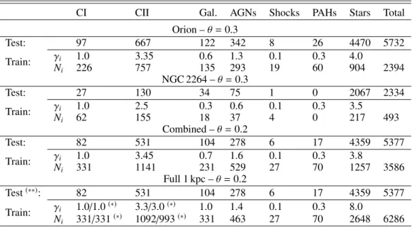
Table 2.Composition of the training and test datasets for each labeled dataset.
CI CII Gal. AGNs Shocks PAHs Stars Total
Orion – θ = 0.3 Test: 97 667 122 342 8 26 4470 5732 Train: γi 1.0 3.35 0.6 1.3 0.1 0.3 4.0 Ni 226 757 135 293 19 60 904 2394 NGC 2264 – θ = 0.3 Test: 27 130 34 75 1 0 2067 2334 Train: γi 1.0 2.5 0.3 0.6 0.1 0.3 3.5 Ni 62 155 18 37 4 0 217 493 Combined – θ = 0.2 Test: 82 531 104 278 6 17 4359 5377 Train: γi 1.0 3.45 0.7 1.6 0.1 0.3 3.8 Ni 331 1141 231 529 27 70 1257 3586 Full 1 kpc – θ = 0.2 Test(∗∗): 82 531 104 278 6 17 4359 5377 Train: γi 1.0/1.0(∗) 3.3/3.0(∗) 1.0 1.4 0.1 0.3 8.0 Ni 331/331(∗) 1092/993(∗) 331 463 27 70 2648 6286
Notes.(∗)The first and second values of γiare for YSOs from the Combined and 1 kpc datasets, respectively.(∗∗)The 1 kpc dataset does not add contaminants, therefore the Full 1 kpc test set is the same as the Combined test dataset to keep realistic observational proportions.
part of the sample was used to build the training and test sets. As discussed below, this was a motivation to repeat the training with various random selections of objects, and thus assess the impact of this random selection on the results.
The adopted values of θ and γi, and the corresponding
num-ber of objects in the training sample are given in Table 2 for each dataset. It shows that with larger labeled datasets we can use smaller values of θ because it corresponds to a large enough number of objects in the associated test set. For the training set of NGC 2264, the number of objects is significantly smaller than in the other datasets, which impacted the results for the associ-ated training. The fine tuning of the γi values is discussed for
each region in Sect.4and a deeper explanation of their impact on the results is given at the end of Sect.3.5.
The results presented in Sects.4and5were obtained using two types of forward datasets. Our main approach was to use the test dataset to perform the forward. In the context of this study, where a label is available for every object and where we are limited by the size of the samples, this allows us to maximize the number of objects in the training set. It does not cause any legitimacy issues because, as explained above, the test set is built with the purpose of being independent of the training dataset and is in observational proportions. To complete our analysis, we also show results obtained by forwarding the complete labeled dataset, to address the effect of the small size of our samples, and to search for hints of over-fitting. We detail this strategy further in Sect.4.1.
Finally, to ensure that our results are statistically robust, each training was repeated several times with different random selec-tions of the testing and training objects based on the θ and γi
factors. This allowed us to estimate the variability of our results, as discussed in Sect. 4. We checked the variability after each change in any of the hyperparameters. In the case of subclasses with many objects, some objects were not included in the train-ing or in the test set. This ensured that the random selection could pick up various combinations of them at each training. In con-trast, in the case of the rare subclasses, since they are entirely included in either the training or the test set, it is more difficult to ensure a large diversity in their selection to test the stability
against selection. For each result presented in Sect. 4we took care to also dissociate this effect from the one induced by the random initialization of the network weights by doing several trainings with the same data selection, which is an indication of the intrinsic stability of the network for a specific set of hyper-parameters.
3.4. Tuning the network hyperparameters
We adjusted most of the network hyperparameters manually to find appropriate values for our problem, in a similar way as illus-trated in AppendixA. To ease the research of optimal values, we started with values from general recipes.
To start, we defined the number of neurons in the hidden layer. The number of neurons can be roughly estimated with the idea that each neuron corresponds at least to a continuous lin-ear separation in the input feature space (Sect. 2.1). Based on Fig.2 at least n = 10 neurons should be necessary since this figure does not represent all the possible combinations of inputs. We then progressively raised the number of neurons and tested whether the overall quality of the classification was improving (Sect.3.5). In most cases it improved continuously and then fluc-tuated around a maximum value. The corresponding number of neurons and the maximum value can vary with the other net-work hyperparameters. The chosen number of neurons is then the result of a joint optimization of the different parameters. We observed that, depending on the other parameters, the average network reached its maximum value for n ≥ 15 hidden neurons when trained on Orion. However, the network showed better sta-bility with a slightly larger value. We adopted n = 20 hidden neurons for almost all the datasets, and increased it to n = 30 for the largest dataset, because it slightly improved the results in this case (Table3). Increasing this number too much could lead to less stability and increases the computation time.
The optimum number of neurons and the maximum quality of the classification also depends on the number of objects in the training dataset. A widely used empirical rule prescribes that the number of objects for each class in the training sample must be an order of magnitude larger than the number of weights in
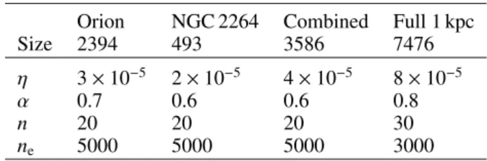
Table 3.Non-structural network hyperparameter values used in training for each dataset.
Orion NGC 2264 Combined Full 1 kpc
Size 2394 493 3586 7476
η 3 × 10⁻⁵ 2 × 10⁻⁵ 4 × 10⁻⁵ 8 × 10⁻⁵
α 0.7 0.6 0.6 0.8
n 20 20 20 30
ne 5000 5000 5000 3000
Notes.The size of the corresponding training set is put for comparison. η is the learning rate, α the momentum, n the number of neurons in the hidden layer, and nethe number of epochs between two control steps. such a network. This means that the minimum size of the train-ing dataset increases with the complexity of the problem ustrain-ing ML algorithms. In our case, including the bias nodes, we would need (m + 1) × n + (n + 1) × o × 10 objects in our training set, with the same notations as in Sect. 2.2. This gives us a mini-mum of 2830 objects in the whole training set using our network structure with n = 20, assuming a balanced distribution among the output classes. As shown in Table 2, some of our training samples are too small for the class I YSOs and critically small for various subclasses of contaminants. Still, each class does not get the same number of neurons from the network. Some classes have a less complex distribution in the parameter space and can be represented by a small number of weights, therefore with fewer training examples. The extra representative strength can then be used to better represent more complex classes that may be more abundant. Thus, it is a matter of balance between having a sufficient number of neurons to properly describe our problem and the maximum amount of available data. This is a strong limitation on the quality of the results.
Our datasets were individually normalized in an interval of −1 to 1, with a mean close to zero for each input feature. This was done for each dimension individually by subtracting the mean value and then dividing by the new absolute maximum value. This evened out the numerical values of the input dimen-sions, which avoided, at the beginning of the training, inappro-priately giving a stronger impact to the dimensions with larger numerical values. Therefore, we set the steepness β of the sig-moid activation of the hidden neurons to β = 1, which worked well with the adopted normalization.
As described in Sect.2.3, we only used the batch CUDA method to train our network throughout this study. We adopted learning rates in the range η = 3−8 × 10⁻⁵ and a momentum
ranging from α = 0.6 to α = 0.8 depending on the dataset, as shown in Table 3. We obtained these values by optimizing the results as illustrated in AppendixA. We note that during training we summed the weight update contributions from each object in the training set (as in, e.g.,Rumelhart et al. 1986b); in order to keep the update values of similar order, the learning rate should be decreased according to the size of the training set (Eqs. (7), and (8)). A variation of this approach could have been employed, where the contributions from each object in the training set would be averaged (as in, e.g.,Glorot & Bengio 2010), sparing the user the necessity of adapting the learning rate to the sample size. This would not change the results since the two strategies are strictly identical with the appropriate choice of learning rate value. Interestingly, we observed for this specific study that the learning rate could instead be slowly increased when the training dataset was larger. This indicates that, in small training sets, the learning process is dominated by the lack of constraints, causing
a less stable value of convergence. This translates into a conver-gence region in the weight space that contains numerous narrow minima due to the larger description granularity of the objects in a smaller dataset. The network can only properly resolve it with a slower learning rate and will be less capable of generaliza-tion. This is an expected issue because we intentionally included small datasets in the analysis to assess the limits of the method with few objects.
Finally, one less important hyperparameter is the number of epochs between two monitoring steps, which was set from ne=
3000 to ne = 5000. It defines at which frequency the network
state is saved and checked, leaving the opportunity to decrease the learning rate η if necessary.
3.5. Representation and quality estimators
In this last part we define the concepts necessary to present our results statistically, and to characterize their quality. For this we use the “confusion” matrix. It is defined as a two-dimensional table with rows corresponding to the original class distribution (targets), and columns corresponding to the classes given to the same objects by our network classification (output). As an exam-ple, Table5shows the 3 × 3 confusion matrix for the Orion test set using observational proportions. This representation directly provides a visual indication of the quality of the network classi-fication. It allows us to define quality estimators for each class. The “recall” represents the proportion of objects from a given class that were correctly classified. The “precision” is a purity indicator of an output class. It represents the fraction of correctly classified objects in a class as predicted by the network. And finally, the “accuracy” is a global quantity that gives the propor-tion of objects that are correctly classified with respect to the total number of objects. In our confusion matrices we show it at the intersection of the recall column and the precision row. Lim-iting the result analysis to this latter quantity may be mislead-ing because it would hide class-specific qualities and would be strongly impacted by the imbalance between the output classes. The matrix format is particularly well-suited to reveal the weak-nesses of a classification. It could, for example, reveal that the vast majority of a subclass goes mistakenly into a specific other subclass, which is informative about any degeneracy between the two classes.
One difficulty highlighted by the use of a confusion matrix is the absence of a global quality estimator since it depends on the end objective. As for any classification problem, one must choose the appropriate balance between reliability and complete-ness. As our aim we chose maximizing the precision for CI, while keeping a large enough value in recall (ideally >90% for both), and a good precision for CII as well. This choice strongly impacts the tuning of the γivalues, since they directly represent
the emphasis given to a class against the others during the train-ing phase, hence biastrain-ing the network toward the class that needs the most representative strength. This will lower the quality of the most dominant objects. A typical example of emphasis on CI YSOs is presented in AppendixAfor the tuning of γStars.
3.6. Convergence criteria
Since training the network is an iterative process, a convergence criteria must be adopted. In principle, this criteria should enable one to identify an iteration where the training has sufficiently converged for the network to capture the information in the train-ing sample, but is not yet subject to over-traintrain-ing. It is customary
Table 4.List of case studies regarding the dataset used to train the network and the dataset to which it was applied to provide predictions. Forward dataset
Orion NGC 2264 Combined Full 1 kpc Training dataset
Orion O–O O–N(∗)
NGC 2264 N–O(∗) N–N
Combined C–C
Full 1 kpc F–C
Notes.(∗)These cases were only forwarded on the full corresponding dataset with no need for a test set. There was no forward on the Full 1 kpc dataset since, as a combination of a complete catalog and a YSO-only catalog, it is not in observational proportions.
to monitor the global error on both the training and test set during the process. While the error of the training set will slowly converge to a minimum value, the error on the test set will fol-low the same curve only for part of the training and then rise when over-fitting begins. However, this global error is affected by the proportions in the training sample and does not neces-sarily reflect the underlying convergence of each subclass. Our approach to this issue was to let the network learn for an obvi-ously unnecessary amount of steps and regularly save the state of the network. This allowed us to better monitor the long-term behavior of the error, and to compare the confusion matrix at regular steps. In most cases the error of the training and test sets both converged to a stable value and stayed there for many steps before the second one started to rise. During this apparently stable moment, the prediction quality of the classes oscillated, switching the classes that get the most representativity strength from the network. Because we want to put the emphasis on CI YSOs, we then manually selected a step that was near the maxi-mum value for CI YSOs precision, with special attention to avoid the ones that would be too unfavorable to CII YSOs.
We observed that the convergence step changed significantly with the network weight random initialization, even with the exact same dataset and network, ranging from 100 to more that 1000, where each step corresponds to several thousands epochs (Table3). Most of the time, the error plateau lasted around 100 steps. We note that the number of steps needed to converge has no consequences on the quality of the results; it only reflects the length of the particular trajectory followed by the network during the training phase.
4. Results
This section presents the YSO classification obtained for the var-ious labeled datasets described in Sect.3. To ease the reading of this section, we summarize all the cases in Table4.
4.1. Results for the Orion molecular cloud
In this section we consider the case where both the training and forward datasets were built from the Orion labeled dataset, here-after denoted the O–O case. The network hyperparameters used for Orion are described in Sect. 3 and Table 3. The resulting confusion matrix is shown in Table5, where the forward set is the test set from Table2, which is in observational proportions. The optimal γi factors found for Orion show a stronger
impor-tance of the CII YSOs (γCII = 3.35) and of the Stars subclass
(γStars = 4.0) than for any other subclass (γi . 1). In contrast,
the optimal values for Shocks and PAHs are saturated in the sense that in Eq. (10), Ntrain
i = (1 − θ) × Nitot, but they appear
to have a negligible impact on the classification quality in this
case. Galaxies and PAHs appear to be easily classified with a rather small number of them in the training sample. This is con-venient since adding too many objects of any class hampers the capacity of the network to represent CI objects (i.e., the most diluted class of interest) in the network, degrading the reliabil-ity of their identification. Therefore, Stars and CII objects could be well represented with a large fraction of them in the training sample, still limiting their number to avoid an excessive dilution of CI YSOs. We note that we have explored different values for the θ parameter. It revealed that the network predictions improve continuously when increasing the number of objects in the train-ing sample. However, to keep enough objects in the test dataset, we had to limit θ to 0.3 (Table2). The only classes for which the number of objects in the training sample is limited by the θ value rather than their respective γivalues are CI YSO, Shocks,
and PAHs. Since Shocks and PAHs are rare in the observational proportions, they are unlikely to have a significant impact on the prediction quality. This leads to the outcome that the following results on Orion are currently limited by the number of CI YSOs in the dataset.
The global accuracy of this case is 98.4%, but the confu-sion matrix (Table5) shows that this apparently good accuracy is unevenly distributed among the three classes. The best rep-resented class is the contaminant class, with an excellent preci-sion of 99.7% and a very good recall of 98.6%. The results are slightly less satisfying for the two classes of interest, with recalls of 90.7% and 97.6%, and precisions of 83.0% and 91.3% for the CI and CII YSOs, respectively. In spite of their very good recall, due to their widely dominant number, objects from the Others class are the major contaminants of both CI and CII YSOs, with 11 out of 18, and 58 out of 62 contaminants, respectively. There-fore, improving the relatively low precision of CI and CII objects mainly requires us to better classify the objects labeled Others. In addition, less abundant classes are more vulnerable to con-tamination. This is clearly illustrated by the fact that the seven CII YSOs misclassified as CI YSOs account for a loss of 7% in precision for CI objects, while the nine CII YSOs misclassified as Others account for a loss of only 0.2% in the Others preci-sion. Those properties are typical of classification problems with a diluted class of interest, where it is essential to compute the confusion matrix using observational proportions. Computing it from a balanced forward sample would have led to apparently excellent results, which would greatly overestimate the quality genuinely obtained in a real use case. It illustrates the necessity of a high γivalue for dominant classes regardless of their interest
(e.g., Stars) as we need to maximize the recall of these classes to enhance the precision of the diluted classes.
To illustrate the interest of selecting our training and test composition with the θ and γi factors, we made a test with a
balanced training set where all three classes were represented by an equal number of objects. The best we could achieve this way
was not more than ∼55% precision on CI YSOs and ∼87% on CII YSO. This was mostly due to the small size of the training sample, which was constrained by the less abundant class, and to the poor sampling of the Others class compared to its great diversity. In contrast, when using our more complex sample def-inition, despite the reduced proportion of YSOs in the training sample, the precision and recall quantities for both CI and CII remained above 80% and 90%, respectively. This means that we found an appropriate balance between the representativity of each class and their dilution in the training sample.
As discussed in Sect. 3.3, we tested the stability of those results regarding (i) the initial weight values using the exact same training dataset, and (ii) the random selection of objects in the training and test set. For point (i) we found that in Orion the weight initialization has a weak impact with approximately ±0.5% dispersion in almost all the quality estimators. For point (ii) we found the dispersion to average around ±1% for the recall of YSO classes. Contaminants were found to be more stable with a recall dispersion under ±0.5%. Regarding the precision value, there is more instability for the CI YSOs because they are weakly represented in the test set and one misclassified object changes the precision value by typically 1%. Overall, we observed values ranging from 77% to 83% for the CI YSOs precision. For the better represented classes we obtained much more stable values with dispersions of ±0.5 to ±1% on class II, and less than ±0.5% on the Others objects. This relative stability is strongly related to the proper balance between classes, controlled by the γi
param-eters, since strong variations between runs imply that selection effects are important, and that there are not enough objects to represent the input parameter space properly.
We also looked at the detailed distribution of classified objects regarding their subclasses from the labeled dataset. These results are shown for Orion in Table 6. It is particularly useful to detail the distribution of contaminants across the three network output classes. For CI YSOs, the contamination appears to originate evenly from various subclasses, while for CII there is a strong contamination from non-YSO stars, though this rep-resents only a small fraction (∼1%) of the Stars population. The distribution of Others objects among the subclasses is very simi-lar to the original (Table1). Interestingly, the Shocks subclass is evenly scattered across the three output classes, which we inter-pret as a failure by the network to find a proper generalization for these objects. More generally, Table6shows that the classes that are sufficiently represented in the training set like AGNs or Stars are well classified, while the Galaxies, Shocks, and PAHs are less well predicted. This is mostly because the training dataset does not fully cover the respective volume in the input parame-ter space or because they are too diluted in the dataset. Addition-ally, Stars and Galaxies mainly contaminate the CII class. This is a direct consequence of the proximity of these classes in the input parameter space, as can be seen in Fig.2.
To circumvent the limitations due to the small size of our test set, we also applied our network to the complete Orion dataset. The corresponding confusion matrix is in Table7, and the asso-ciated subclass distribution is in Table8. It may be considered a risky practice because it includes objects from the training set that could be over-fitted, so it should not be used alone to ana-lyze the results. Here, we use it jointly with the results on the test set as an additional over-fitting test. If the classes are well constrained, then the confusion matrix should be stable when switching from the test to the complete dataset. For Orion we see a strong consistency between Tables5and7for the Others and CII classes, both in terms of recall and precision. For CI YSOs, the recall increases by 3.4%, and the precision decreases
Table 5.Confusion matrix for the O–O case for a typical run. Predicted
Class CI YSOs CII YSOs Others Recall
CI YSOs 88 4 5 90.7%
Actual CII YSOs 7 651 9 97.6%
Others 11 58 4899 98.6%
Precision 83.0% 91.3% 99.7% 98.4%
Table 6.Subclass distribution for the O–O case. Actual
CI CII Gal AGNs Shocks PAHs Stars
CI 88 7 1 2 3 3 2
Predicted CII 4 651 5 0 2 4 47 Others 5 9 116 340 3 19 4421
Table 7.Confusion matrix for the O–O case forwarded on the full dataset.
Predicted
Class CI YSOs CII YSOs Others Recall
CI YSOs 305 11 8 94.1%
Actual CII YSOs 34 2157 33 97.0% Others 34 201 16331 98.6% Precision 81.8% 91.1% 99.7% 98.3%
Table 8.Subclass distribution for the O–O case forwarded on the full dataset.
Actual
CI CII Gal AGNs Shocks PAHs Stars
CI 305 34 2 11 11 7 3
Predicted CII 11 2157 10 9 9 18 155 Others 8 33 395 1121 8 62 14745 by 1.2%. These variations are of the same order as the vari-ability observed when changing the training set random selec-tion, indicating that fitting is unlikely here. If there is over-fitting it should be weak and restricted to CI YSOs. Therefore, the results obtained from the complete Orion dataset appear to be reliable enough to take advantage of their greater statistics. Table7gives slightly more information than Table5, and mostly confirms the previous conclusions on the contamination between classes. Table8provides further insight. AGNs, which seemed to be almost perfectly classified, are revealed to be misclassified as YSOs in 1.8% of cases. It also shows that the missed AGNs are equally distributed across the CI and CII YSO classes. Shocks are still evenly spread across the three output classes. Regarding PAHs, Table8reveals that there is more confusion with the CII YSOs than with the CI YSOs.
4.2. NGC 2264 open cluster
For this section we used the training and forward datasets for NGC 2264 described in Table 2 with the corresponding
hyperparameters (Table 3). The results for this region alone, obtained by a forward on the test set, are shown in Table9, with the subclass distribution in Table 10. We refer to this case as the N–N case. The major differences with Orion are expected to come from the differences in input parameter space coverage and from the different proportions of each subclass. This N–N case is also useful to see how difficult it is to train our network with a small dataset. The recall and precision of CI YSOs are greater (96.3% and 89.7%, respectively) than in Orion, but the corresponding number of objects is too small to draw firm con-clusions. For CII YSOs, the recall and precision are less than in Orion by approximately 4% and 10%, respectively. The Others class shows similar values to those in Orion.
We highlight here how having a small learning sample is problematic for this classification. First of all, the training set contains only 62 CI YSOs, which is far from enough in regard of the size of the network (Sect.3.4). This difficulty is far worse than for Orion because, to avoid dilution, we had to limit the number of objects in the two other classes, leading to the small size of the training sample (493 objects), and consequently to worse results for all classes. To mitigate these difficulties and because the dilution effect occurs quickly, we adopted lower γi values for CII YSOs and Stars, thus reducing their relative
strength. It results in too small training set sizes for all the sub-classes compared to the number of weights in the network. How-ever, we observed that a decrease in the number of neurons still reduced the quality of the results. Although a lower number of hidden neurons tended to increase stability, we chose to keep them at n = 20 to get the best results and to reduce the learn-ing rate to achieve better stability. We note that, due to the use of batch training, the smaller size of the dataset than for the O– O case is equivalent to an additional lowering of the learning rate because the typical magnitude of the weight updates scales with the batch size (Sect.2.3). For this dataset slight changes in the γi values happened to lead to great differences in terms of
results and stability, which is a hint that the classification lacks constraints.
Even for a given good γi set, there is a large scatter in the
results when changing the training and test set random selec-tion. It leads to a dispersion of about ±4% in both recall and precision for the CI YSOs. This can be due to a lack of represen-tativity of this class in our sample, but it can also come from small-number effects in the test set that are stronger than in Orion. These two points show that the quality estimators for CI YSOs are not trustworthy with such a small sample size. The results shown in Tables9 and10correspond to one of the best trainings on NGC 2264, that achieves nearly the best val-ues for CI quality estimators. The CII precision dispersion is about ±2%, and its average value is around 80%, which is higher than in the specific result given in Table9, but still significantly lower than for Orion. In contrast, the CII recall is fairly stable with less than ±1% dispersion. Contaminants seem as stable as for Orion using these specific γivalues. However, it could come
from the artificial simplification of the problem due to the quasi-absence of some subclasses (Shocks and PAHs; see Table2) in the test set. We note that the network would not be able to clas-sify objects from these classes if this training were applied to any other region that contained such objects.
As in the previous section, we studied the effect of the ran-dom initialization of the weights. We found that both precision and recall of YSO classes are less stable than for the O–O case with a dispersion of ±1.5% to ±2.5%. The Others class shows a similar stability to that for Orion, with up to ±0.5% dispersion on precision and recall, which could again be biased by the fact
Table 9.Confusion matrix for the N–N case for a typical run. Predicted
Class CI YSOs CII YSOs Others Recall
CI YSOs 26 1 0 96.3%
Actual CII YSOs 1 121 8 93.1%
Others 2 31 2144 98.5%
Precision 89.7% 79.1% 99.6% 98.2%
Table 10.Subclass distribution for the N–N case. Actual
CI CII Gal AGNs Shocks PAHs Stars
CI 26 1 0 2 0 0 0
Predicted CII 1 121 4 5 1 0 21 Others 0 8 30 68 0 0 2046
Table 11.Confusion matrix for the N–N case forwarded on the full dataset.
Predicted
Class CI YSOs CII YSOs Others Recall
CI YSOs 88 2 0 97.8%
Actual CII YSOs 7 406 22 93.3%
Others 12 77 7175 98.8%
Precision 82.2% 83.7% 99.7% 98.4%
Table 12.Subclass distribution for the N–N case forwarded on the full dataset.
Actual
CI CII Gal AGNs Shocks PAHs Stars
CI 88 7 0 8 3 0 0
Predicted CII 2 406 8 10 1 0 58 Others 0 22 106 232 2 0 6835 that the absence of some subclasses simplifies the classification. These results indicate as before that our network is not suffi-ciently constrained using this dataset alone with respect to the architecture complexity that is needed for YSO classification.
The forward on the complete NGC 2264 dataset is crucial in this case since it may overcome small-number effects for many subclasses. The corresponding results are shown in Tables 11
and 12. It is more difficult in this case than for O–O to be sure that there is no over-training, even with a careful moni-toring of the error convergence on the test set during the train-ing, because the small-number effects are important. As a pre-caution, in all the results for the N–N case, we chose to stop the training slightly earlier in the convergence phase in com-parison to Orion, for which we found over-training to be neg-ligible or absent (Sect. 4.1). We expect this strategy to reduce over-training, at the cost of a higher noise. With this assumption, the results show more similarities to the Orion case than those obtained with the test set only (comparing Tables 7 and 11). Because NGC 2264 contains fewer CI and CII YSOs than Orion, their boundaries with the contaminants in the parameter space