Distributional Effects of Net Metering Policies and
Residential Solar Plus Behind-the-meter Storage
Adoption
by
Andrés Inzunza Besio
B.S. Industrial Engineering (2011)
M.S. Electrical Engineering (2014)
Pontificia Universidad Católica de Chile
Submitted to the Institute for Data, Systems, and Society
in partial fulfillment of the requirements for the degree of
Master of Science in Technology and Policy
at the
MASSACHUSETTS INSTITUTE OF TECHNOLOGY
May 2020
c
○ Massachusetts Institute of Technology 2020. All rights reserved.
Author . . . .
Institute for Data, Systems, and Society
May 8, 2020
Certified by . . . .
Christopher Knittel
George P. Shultz Professor of Applied Economics
Thesis Supervisor
Accepted by . . . .
Noelle Selin
Director, Technology and Policy Program
Associate Professor, Institute for Data, Systems, and Society and
Department of Earth, Atmospheric and Planetary Sciences
Distributional Effects of Net Metering Policies and
Residential Solar Plus Behind-the-meter Storage Adoption
by
Andrés Inzunza Besio
Submitted to the Institute for Data, Systems, and Society on May 8, 2020, in partial fulfillment of the
requirements for the degree of
Master of Science in Technology and Policy
Abstract
Several authors argue that net metering schemes (NEM), typically implemented to incentivize investment on distributed energy resources (DER), could be regressive, given that DER adopters in the U.S. are wealthier on average than non-adopters and due to the possibility that DER owners shift certain costs onto passive customers. By using a dataset containing close to 100,000 customers’ half-hourly load data and income quintiles from Chicago, IL, we simulate the operation of residential solar and behind-the-meter battery systems under 20%, 45% and 70% adoption levels and cal-culate both resulting bills for every client in the dataset, as well as cost shifts arising from the combination of NEM and the allocation of network and policy costs (i.e., residual costs) through volumetric charges (i.e., in $/kWh). Additionally, we con-sider different tariff designs. Results show that the combination of NEM schemes and recovery of residual costs through volumetric charges may cause important cost shift-ing effects from DER adopters onto non-adopters, risshift-ing equity and fairness concerns. Firstly, under NEM schemes, we calculate that adopter customers may, on average, obtain bill reductions of 71% when installing solar or solar plus storage, whereas non-adopters can see their bills increased 18% in high DER penetration scenarios (i.e., 45% penetration). Moreover, under the same NEM schemes, 45% adoption and considering solar plus storage adoption alone, we calculate that customers from the two lowest income quintiles may suffer bill increases in the 16-19% range on average, while removing NEM schemes reduces these increases to the 11-12% range.
Thesis Supervisor: Christopher Knittel
Acknowledgments
This work would not have been possible without the advances of several people. In particular, I would like to thank Scott Burger for his notable contributions through his PhD dissertation and his guidance throughout the development of this thesis.
Furthermore, I owe much to my advisor, Professor Christopher Knittel for his overall support during my studies at MIT. Working as a research assistant with him was an invaluable experience in my career, and I owe him, among others: my newly-found interest in econometrics and data science in general; many fun and educational lunches at CEEPR, which I count among the best experiences I had at MIT; and the freedom to research topics of my own choosing. Thank you so much for everything Chris and I really hope we continue working together. #taxcarbon.
I also feel incredibly fortunate for having met my classmates at the Technology and Policy Program. I was continuously amazed and inspired by their kind-heartedness, brilliance and passion for creating positive impact. I truly hope the program continues gathering people like them, who have this great combination of childish curiosity, geeky love for rigorous work and the drive to actually try to change the world.
I also owe much to my Chilean family in Boston and the many latins with whom Fernanda and I became so close (Augusto, Lorena, Armando, Pati and many others). Ustedes le dieron sabor y color a nuestra vida en MIT. ¡Los queremos mucho!
Finally, I would like to thank the four most important people in my life. My parents, my brother and my future wife, Fernanda. You are my foundation, all my accomplishments are yours as well.
Contents
1 Introduction 12
1.1 The challenge of designing electricity tariffs. . . 15
1.1.1 Achieving economically efficient and revenue-sufficient electric-ity tariffs. . . 16
1.1.2 Achieving equitable and/or fair electricity tariffs . . . 20
1.2 Net metering schemes: Definitions, objectives and controversies . . . 22
1.3 State-of-the-art and contributions of this work . . . 24
2 Methodology 28 2.1 General description of the methodology . . . 28
2.2 Customer data description . . . 32
2.3 DER adoption probability . . . 32
2.4 Tariff designs and NEM regimes . . . 34
2.5 Solar generation modeling . . . 37
2.6 Storage operation modeling . . . 38
2.6.1 Mathematical formulation for NEM "On" and NEM "Off" regimes 39 2.6.2 Mathematical formulation for the NEM "On-California" regime 41 2.6.3 Assumptions. . . 42
3 Results and Discussion 43 3.1 DER adoption by quintile and illustrative operation results . . . 43
3.2 NEM policies benefit adopter customers while shifting costs onto non-adopters, rising equity concerns . . . 47
3.3 Removing NEM regimes improves fairness of tariff designs . . . 52
3.4 Removing NEM regimes improves economic value of storage for adopters 55
3.5 Depending on the tariff design, presence/absence of NEM regimes changes grid usage considerably under high DER penetrations . . . . 58
4 Conclusion 64
Bibliography 66
Appendices 71
A Additional results for 90% (base case) of solar energy offset
assump-tion 71
A.1 Bill impacts on adopters and non-adopters under all tariff designs and DER penetration levels . . . 71
A.2 Bill impacts on non-adopters under ToU tariff and 20% and 70% adop-tion levels by income quintile . . . 72
A.3 Bill impacts on non-adopters under flat, RTP and RTP-Efficient tariffs and 45% adoption level . . . 74
B Bill impacts on non-adopters for 70%, 90% (base case) and 110% of
solar energy offset assumption 76
List of Figures
1-1 Economically efficient and revenue-sufficient charges for allocating net-work costs (MIT Energy Initiative, 2016). . . 19
1-2 Net metering schemes in the U.S. (NC Clean Energy Technology Cen-ter, 2019). . . 23
2-1 Time-of-use charges periods as defined by ComEd in its RTOUPP tariff. 35
2-2 Time-of-use charges that include energy and capacity costs.. . . 36
2-3 Real time pricing charges that include energy and capacity costs (hourly average). . . 36
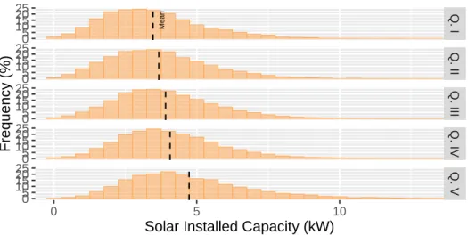
3-1 Solar installed capacity for each adopter customer in the 70% DER adoption scenario.. . . 44
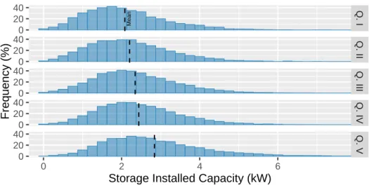
3-2 Storage installed capacity for each adopter customer in the 70% DER adoption scenario.. . . 45
3-3 Hourly average of DER operation for a particular customer. . . 46
3-4 Hourly average of load and net load for a particular customer (same customer as figure 3-3). . . 47
3-5 Mean bill change for DER adopters under different adoption levels (compared to the no adoption scenario), considering solar adoption alone and time-of-use tariffs. . . 48
3-6 Mean bill change for DER adopters under different adoption levels (compared to the no adoption scenario), considering solar plus storage adoption alone and time-of-use tariffs.. . . 49
3-7 Mean bill change for non-adopters under different adoption levels (com-pared to the no adoption scenario), considering solar adoption alone and time-of-use tariffs. . . 49
3-8 Mean bill change for non-adopters under different adoption levels (com-pared to the no adoption scenario), considering solar plus storage adop-tion alone and time-of-use tariffs. . . 50
3-9 Mean bill change for non-adopters under different tariff designs (com-pared to the no adoption scenario), considering solar plus storage adop-tion alone and 45% penetraadop-tion. . . 51
3-10 Mean bill change for non-adopters under different tariff designs (com-pared to the no adoption scenario), considering solar plus storage adop-tion alone and 45% penetraadop-tion. . . 52
3-11 Bill impacts of DER adoption on non-adopters by income quintile and NEM regime, calculated using the Time-of-use tariff and 45% of solar plus storage adoption. . . 53
3-12 Mean bill increase for non-adopters, normalized by quintile mean in-come assuming a 45% adoption level of solar plus storage. . . 54
3-13 Marginal revenues (i.e., economic value) for solar adopters, triggered by installing storage under different tariff designs. . . 55
3-14 Cumulative frequency of the per-kWh economic value of storage. . . . 57
3-15 Marginal revenues (i.e., economic value) for solar adopters, triggered by installing storage under different NEM regimes and tariff designs.. 58
3-16 Excess load compared to original total load and negative load (or ex-ports to the grid from customers) for all NEM regimes, different solar plus storage adoption levels and flat tariff. . . 59
3-17 Excess load compared to original total load and negative load (or ex-ports to the grid from customers) for all NEM regimes, different solar plus storage adoption levels and ToU tariff. . . 61
3-18 Excess load compared to original total load and negative load (or ex-ports to the grid from customers) for all NEM regimes, different solar plus storage adoption levels and RTP tariff. . . 62
3-19 Excess load compared to original total load and negative load (or ex-ports to the grid from customers) for all NEM regimes, different solar plus storage adoption levels and RTP-Efficient tariff. . . 63
A-1 Mean bill change for DER adopters under different adoption levels (compared to the no adoption scenario) and tariff designs. . . 71
A-2 Mean bill change for non-adopters under different adoption levels (com-pared to the no adoption scenario) and tariff designs. . . 72
A-3 Bill impacts of DER adoption on non-adopters by income quintile and NEM regime, calculated using the Time-of-use tariff and 20% of solar plus storage adoption. . . 73
A-4 Bill impacts of DER adoption on non-adopters by income quintile and NEM regime, calculated using the Time-of-use tariff and 70% of solar plus storage adoption. . . 73
A-5 Bill impacts of DER adoption on non-adopters by income quintile and NEM regime, calculated using the flat tariff and 45% of solar plus storage adoption. . . 74
A-6 Bill impacts of DER adoption on non-adopters by income quintile and NEM regime, calculated using the RTP tariff and 45% of solar plus storage adoption. . . 75
A-7 Bill impacts of DER adoption on non-adopters by income quintile and NEM regime, calculated using the RTP-Efficient tariff and 45% of solar plus storage adoption. . . 75
B-1 Mean bill change for non-adopters (compared to the no adoption sce-nario) under different adoption levels, tariff designs and solar energy offset assumption for the NEM On case. . . 76
B-2 Mean bill change for non-adopters (compared to the no adoption sce-nario) under different adoption levels, tariff designs and solar energy offset assumption for the NEM On-California case. . . 77
B-3 Mean bill change for non-adopters (compared to the no adoption sce-nario) under different adoption levels, tariff designs and solar energy offset assumption for the NEM Off case. . . 77
List of Tables
2.1 Number of customers by income quintile and Delivery Service Class in the dataset used for calculations. . . 33
2.2 Distribution of solar PV adopters in the U.S. by quintile in 2016 (Bar-bose et al., 2018). . . 33
2.3 Tariff designs and cost allocations considered in the present study. . . 34
2.4 Tariff designs and cost allocations considered in the present study. . . 35
Chapter 1
Introduction
Given that electricity markets may involve a mix of regulated and competitive activ-ities, prices (or tariffs) paid by end-consumers can be composed by the combination of regulated and unregulated charges.12 In general, procedures used in jurisdictions
to set regulated tariffs3 that will then be passed on to consumers follow roughly the
following steps:
Firstly, the total amount of revenues that companies are allowed to collect from customers in a certain period is determined4, given their (approved) costs and a
regulated rate-of-return. This process varies widely across jurisdictions, and many approaches have been proposed in order to provide efficiency incentives to companies while maintaining a reasonable regulatory cost (Pérez-Arriaga, 2013).
Secondly, the structure of the tariff is set. This entails, for instance, deciding whether tariffs would vary across time or point of connection; if tariffs would change across customer classes; if they would involve a fixed charge, a volumetric charge –in $/kWh- and/or a capacity charge –in $/kW-, etc.
1E.g., Texas, Massachusetts, Australia, the U.K. and others (M. J. Morey and L. D. Kirsch,
2016).
2In other cases e.g., Chile, most of California and others., even when some activities have been
deregulated (e.g., generation), the tariff that end-consumers pay is completely determined or ap-proved by the regulator.
3Either those that remunerate only regulated activities or those that will remunerate the complete
electricity value chain.
4E.g., in the case of distribution companies a period of 4-8 years is common, which is called “price
Finally, the third step consists in deciding which types of the company’s costs will be allocated to each element of the designed structure (Pérez-Arriaga, 2013).
In the face of a widespread penetration of distributed energy resources (DER) in electric grids, such as residential solar PV, batteries, electric heat pumps, etc., an inadequate tariff design (second and third steps) may have uneven consequences across different socioeconomic groups. In the U.S., owners of residential solar systems are wealthier than non-owners, given that more than 80% of solar owners belong to the top 3 income quintiles (Barbose et al., 2018). If, for instance, an important portion of utilities costs are collected through the volumetric charge of tariffs, solar adopters, whose electricity consumption from the grid is lower, would contribute less to paying for the electric infrastructure (e.g., networks), and thus, uncollected revenues would have to be obtained from other customer groups (S. Burger et al.,2019).
Moreover, other types of DERs, such as behind-the-meter (BTM) batteries, could provide an even greater opportunity to reduce electricity bills paid by adopter clients (Hledik & Greenstein, 2016). These resources allow the consumer to manage the amounts of electricity they consume from the system flexibly and could be used to further optimize their consumption. For instance, battery adopters might be able to increase their consumption in low rate hours and decrease it during times in which tariffs are higher. In addition, battery adopters might be able to reduce overall peak demand, which in some cases is subject to additional charges. In any case, batteries grant consumers greater flexibility to respond to price signals, which makes tariff design even more important in these cases.
Adding further complexity to the context, net metering (NEM) schemes are widely adopted in the U.S. and around the world in order to incentivize investment on resi-dential solar PV systems and more recently, on behind-the-meter storage (California Public Utilities Commission,2019; The Commonwealth of Massachusetts Department of Public Utilities, 2019). Under the most simple definition, these schemes consist on valuing net imports (i.e., consumption) and net exports of power from customers premises to the grid5 at the full retail tariff.
In many jurisdictions in the U.S. and other countries, an important fraction of network costs are recovered through volumetric charges (Brown & Faruqui, 2014). Hence, given that NEM policies help DER adopters avoiding some of these costs, we argue that these policies may increase undesireable distributional impacts of DER adoption6, under some tariff designs.
In this context, the present work aims at answering the following research ques-tions:
i. How do different tariff designs combined with NEM schemes interact with differ-ent levels of solar PV and BTM storage adoption, in terms the economic impact on adopters and non-adopters of DER?
ii. How would the benefits and costs of solar and storage adoption be distributed across different income quintiles?
iii. How do different tariff designs combined with NEM schemes and solar plus stor-age adoption interact with other aspects relevant to policy making, such as the economic value that adopters draw from the adoption of BTM storage and po-tential costs/benefits due to increased/decreased needs regarding network assets? To answer these questions we structure the present document as follows:
∙ The following sections in the present chapter summarize the theoretical back-ground on tariff design and current open questions in the literature regarding equity and fairness concerns in the subject.
∙ Chapter 2 details methods used in this work: Data; assumptions; and mathe-matical formulation of models used.
∙ Chapter 3 summarizes results and provides the corresponding analysis. ∙ Chapter 4 provides the concluding remarks and implications of our work.
6I.e., benefiting high-income consumers which are normally the ones that adopt DER, allowing
1.1
The challenge of designing electricity tariffs
As explained above, designing electricity tariffs entails deciding the format or struc-ture as well as the cost streams allocated to each type of charge in the tariff, for each consumer. This is in essence, a complex7 problem, since there are several, and sometimes competing objectives that a tariff design must comply with in order to be reasonably adequate for implementation and gain social acceptance.
Bonbright, 1962 is often cited as the seminal work in which the objectives or principles of tariff design were established. Later on, (Pérez-Arriaga, 2013) and oth-ers (e.g., (Rábago & Valova, 2018)) have continued to clarify and re-interpret these principles and adapt them to contemporary contexts. In any case, there are three primarily relevant principles that are common to these works: (1) revenue sufficiency (i.e., the ability of the tariff design to collect the revenues required or approved for the utility and remunerate the activity adequately); (2) equitable and fair allocation of costs across customer classes; and (3) economic efficiency (i.e., provide incentives so products are consumed by whoever benefits most from them). Other principles estab-lished by previously mentioned works are transparency, simplicity, stability, among others. In the present work, we concentrate on the first three.
Although not necessarily an easy task, there are several comprehensive works that provide guidance on how to achieve economically efficient (and revenue-sufficient) tariffs for the electricity service8. However, achieving a fair and/or equitable allocation
of costs seems to be an open problem both in the academic and policy-making arenas (S. P. Burger et al., 2020). The following sections of this work aim at summarizing state-of-the-art recommendations for achieving economically efficient and revenue-sufficient electricity tariffs and present the main challenges that arise when dealing with equity and fairness issues.
7Or "wicked", as defined by (Rittel & Webber,1973).
8E.g., see (Borenstein,2016b; S. Burger et al., 2019; Hogan, 2013; MIT Energy Initiative, 2016;
1.1.1
Achieving economically efficient and revenue-sufficient
electricity tariffs
In this work we assume that tariffs should recover the costs that remunerate the whole electricity value chain. In this context, a revenue-sufficient electricity tariff should collect from end-consumers the whole range of cost streams that stem from the electricity service: Those related to electricity generation (i.e., energy, capacity and ancillary services), network investments and operation (i.e., transmission and distribution grids), electricity losses in all previous processes and any other costs that are assigned to the electricity service.9
In terms of economic efficiency, the guiding principle is to charge consumers as close as possible to the short-term marginal cost of their consumption (Borenstein,
2016b; Pérez-Arriaga, 2013). As we will see ahead in this section, there are several reasons why tariffs solely based on short-run marginal costs will not be sufficient to pay for the complete supply chain of the electric service. In these cases, tariffs should be complemented by other charges that can, in theory, minimize deadweight loss of departing from marginal cost pricing (Borenstein, 2016b).
In the case of the generation segment, there are three main cost streams that should be allocated onto the final consumer: the marginal cost of generated energy10, capacity costs and ancillary services.
The marginal cost of energy, varies over time11and throughout the different nodes in the system due to losses and network congestion. Ideally, this cost should be included in tariffs through a volumetric charge (in $/kWh) that mimics as close as possible the short-run marginal cost of producing and delivering electric energy to the consumer at all times and throughout all nodes in the system (S. Burger et al.,
2019; MIT Energy Initiative, 2016). In reality, the latter can be difficult due to
9For instance, in many jurisdictions, costs of several policies related or unrelated to the electricity
service are incorporated in end-consumer tariffs (MIT Energy Initiative,2016).
10Captured by the wholesale price of energy in deregulated markets.
11Due to demand levels, available generation, network constraints and losses stemming from power
implementation costs12 or fairness considerations.1314
Capacity costs arise in certain markets as a consequence of capping the maximum value that the short-run marginal cost of energy can take, among other practical reasons (Joskow, 2008). This is a common practice among regulators and it is done in jurisdictions such as California, the Pennsylvania, Jersey, Maryland Power Pool (PJM), Chile, U.K., and others. Given this price cap, sales of energy in the wholesale market are insufficient to remunerate investment and operating costs of a sufficiently reliable electricity service (Joskow, 2008). Consequently, these markets need some form of capacity payment or capacity market to make the market whole.
These capacity costs are driven mainly by the aggregated impact of customers consumption decisions on future investments on generation capacity and thus, an economically efficient charge should take the form of a peak-coincident demand charge (S. Burger et al.,2019). This type of charges can be included in final tariffs through a $/kW term and should capture the extent to which each consumers’ load contributes to the overall demand peak that may trigger the need for generation investments.
Operating reserves and other ancillary services15tend to represent a small fraction
of generation costs (1-2%) according to some authors (MIT Energy Initiative, 2016), however, they can still provide an attractive business opportunity for distributed energy resources. Costs that stem from these services are varied and, given their relative low value, they tend to be averaged and added as an uplift to volumetric charges in end-user tariffs. Recommendations in the literature suggest that at least, these costs should be conveyed with higher time and spatial granularity (MIT Energy Initiative, 2016), in order to capture more accurately the value/costs that DER and consumers’ actions may add to the system in terms of requirements for ancillary
12Given that highly granular price signals need advanced IT infrastructure to be deployed, both
to deliver the signal to the end-consumer and to allow them to react to these prices.
13E.g., poor consumers living in rural areas with high losses may be subject to very high marginal
costs of energy.
14In practice, policy-makers can resort to approximations to these ideal time and spatially-granular
energy prices, such as time-of-use tariffs and zonal locational marginal prices (LMP) and gradually move forward with the implementation of more efficient price signals (see (MIT Energy Initiative, 2016) for further detail).
services.
In the case of network costs (transmission and distribution investment and op-eration), it is a widely accepted fact that it is impossible to recover them resorting solely on pricing on the basis of marginal costs. Although there are several reasons for this, the primary causes of this effect are a combination of the discrete character of investments in network assets and the presence of steep economies of scale (Pérez-Arriaga,2013). The lumpiness in network investments triggers a sustained difference between the optimally adapted network16and the real one, given that network assets
will tend to go through an over-investment cycle earlier on their lifetime, depressing marginal cost-based price signals. Moreover, the presence of economies of scale makes it more efficient to perform larger investments at once, rather than building smaller and more incremental network assets on a more gradual basis. The latter increases the tendency to have an over-dimensioned grid, which in turn reduces marginal cost prices even more.
Given the latter, ideally, network costs can still be allocated using a combination of marginal cost-based prices and other measures that can reduce the economically inefficient effects of non-marginal pricing.
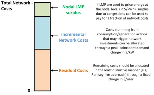
Figure 1-1 shows recommendations by (S. Burger et al.,2019; MIT Energy Initia-tive,2016). As shown in the figure, if nodal locational marginal prices are available17, network energy losses and congestions may trigger differences on these LMP measured at the different sides of a transmission line or a distribution feeder. Consequently, differences of power injections and withdrawals in the line, valued at LMP, can be high enough to pay for energy losses and part of investment and operation costs of the asset.
Nodal LMP (either at the transmission or distribution levels) can, in theory, cap-ture well the marginal effects of consumption and generation decisions on the short-term operation of the power system (Hogan, 2013). However, due to the causes
16I.e., the one that under ideal conditions would make marginal price signals high enough to pay
for all network costs.
explained earlier18 these signals fail to capture the long-term marginal effects of these decisions19. Some authors argue that the latter can be captured by peak-coincident
demand charges (S. Burger et al.,2019; MIT Energy Initiative, 2016). As in the case of capacity costs, these charges can be added to the final tariff in $/kW, however in this case, ideally, the magnitude of the charge should convey the contribution of consumption/generation peaks to the need for future network investments.
If LMP are used to price energy at the nodal level (in $/kWh), surplus due to congestions can be used to pay for a fraction of network costs
Costs stemming from consumption/generation actions
that may trigger network investments can be allocated through a peak-coincident demand
charge in $/kW Nodal LMP surplus Incremental Network Costs Residual Costs 0 -Total Network Costs
-Remaining costs should be allocated in the least distortive manner (e.g. Ramsey-like approach) through a fixed
charge in $/user
Figure 1-1: Economically efficient and revenue-sufficient charges for allocating net-work costs (MIT Energy Initiative,2016).
As shown in figure 1-1, after collecting revenues stemming from nodal LMP and forward-looking demand charges, there may be costs yet to be recovered to make investors whole. These costs are typically labelled as residual and it is very difficult to devise a way of allocating them, given that they are not "caused" by any identifiable action of any agent in the system. Other costs typically allocated onto the electricity bill, such as the cost of environmental policies or other public policies face the same issues (MIT Energy Initiative, 2016).
If only economic efficiency is the concern, then the literature suggests that a
cri-18E.g., economies of scale, lumpiness of network investments and others.
terion based on Ramsey pricing could be used.20 This entails assigning residual costs as fixed charges ($/consumer) inversely to wealth demand elasticity21 of consumers.
This way, consumers that value electricity higher will pay more and deadweight loss, in theory, would be minimized (Borenstein,2016b; S. Burger et al.,2019; MIT Energy Initiative, 2016). In practice, the strict application of the principle can be unfeasi-ble both due to fairness concerns and the difficulty of estimating consumer demand elasticity. Still, this criterion has been applied to some extent when utilities provide discount rates to commercial and industrial customers who can move their operations to alternative jurisdictions (Borenstein, 2016b). Consequently (and ignoring fairness concerns for now), some form of proxy for demand elasticity could be used in practice to set rates using the Ramsey rationale.
1.1.2
Achieving equitable and/or fair electricity tariffs
The concepts of equity and fairness are yet to be definitely defined in the energy economics and policy arena. However, in order to maintain a clear division across both concepts and their underlying importance in tariff design, we will use definitions provided by (S. Burger et al., 2019).
Equity is understood in this work as allocative equity as defined by (S. Burger et al., 2019). Authors of this work define allocative equity as:
"(...) we define an allocatively equitable tariff as a tariff that treats identical customers equally (...). In practice, this has two key implications:
1. Marginal consumption or production decisions are charged or paid according to the marginal costs or values they create.
2. Residual costs are allocated according to customer characteristics that are not im-pacted by their short term electricity consumption or production decisions. In other words, one customer’s behavior cannot cause another customer to pay more or less residual costs."
20See (Ramsey,1927) for the original application of Ramsey pricing in the context of taxation. 21I.e., the change on electricity demand due to a change in wealth.
Firstly, note that (S. Burger et al., 2019) consider identical consumers to be the ones that make identical power consumption/generation decisions22, which entails as
a corollary, that demand elasticity could play a role in the definition of identical customers. As a consequence, a Ramsey criterion to allocate residual costs can be considered equitable under this definition.
Secondly, we underscore that an important consequence of this definition of equity, is that an equitable tariff would minimize residual costs shifts between customers.
Consequently, under this definition of equity, we can safely assume that more economically efficient tariffs will also be more equitable. As demonstrated by (S. Burger et al., 2019) using flat volumetric tariffs as a base case, more economically efficient tariffs would always reduce cross subsidies of marginal costs and cost shifts of residual costs between customers, improving equity as understood here.
Following (S. Burger et al.,2019) definition for a fair (or distributionally equitable) tariff, we understand the concept as "(...) a tariff structure (...) (that) meets locally defined standards of social justice with respect to the distribution of goods between vulnerable and non-vulnerable customers".
Under this definition of fairness, it is impossible to state that economically efficient tariffs would also maximize fairness, given that fairness as defined here obeys to locally defined standards of social justice which are inherently subjective. For instance, under the strict application of Ramsey criterion for the allocation of residual costs (which is both economically efficient and equitable), low-income customers that use electricity only for basic needs would pay proportionally more than wealthier customers using electricity for leisure activities, effect that could clearly be deemed to be unfair by some.
Although several customer characteristics may be used to define social justice standards and vulnerability, in this document we concentrate on income and how different tariff designs affect low-income customers (i.e., vulnerable).
1.2
Net metering schemes: Definitions, objectives
and controversies
Net metering is a broad term when considering the specifics of each application23,
however, in general it refers to a scheme where customers that have installed gen-eration assets (in most cases PV systems) are billed on the basis of the net energy they consume by the end of the billing period.24 The underlying mechanics of the strict application of this definition, imply that injections of power to the grid are valued at exactly the same price as power consumption. In contrast, other schemes such as net billing25, consist on valuing net injections of power at a reduced monetary
value compared to the full retail tariff, under the assumption that injections of power should not avoid certain costs, such as residual network or policy costs.
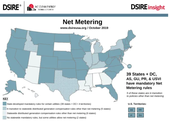
Probably due to its simplicity, net metering is widely used in the U.S. and many other countries as a way to incentivize investments in residential solar and, more recently, on BTM storage. In effect, Figure 1-2 shows the adoption of NEM schemes across the different states in the U.S., where almost 80% of states have implemented mandatory NEM schemes for certain utilities.
Moreover, NEM schemes that have historically been applied mostly to incentivize investment in solar PV in the U.S. have been more recently extended to BTM storage. In January 2019 California issued a decision to extend net metering to solar plus storage facilities, as long as energy generated by storage assets is provided by the solar system (and not from the grid) (California Public Utilities Commission, 2019). A month afterwards, Massachusetts issued a similar decision, where it allowed BTM storage owners to be included in the state’s NEM scheme, as long as the power generated by the assets is charged by a net metering facility (e.g., solar system) or charged from the grid but the storage system is unable to export to the grid (The Commonwealth of Massachusetts Department of Public Utilities, 2019).
It is important to note that under a net metering scheme and flat two-part
tar-23See for instance, (Hughes & Bell,2006).
24That is, all energy used at their premises, minus energy generated by their generation assets. 25See (Zinaman et al.,2017) for an overview of different metering and billing arrangements.
Net Metering
State-developed mandatory rules for certain utilities (39 states + DC+ 4 territories)
Statewide distributed generation compensation rules other than net metering (6 states)
www.dsireusa.org / October 2019
KEY
U.S. Territories:
39 States + DC, AS, GU, PR, & USVI have mandatory Net Metering rules
DC
No statewide mandatory rules, but some utilities allow net metering (2 states)
GU AS PR VI In transition to statewide distributed generation compensation rules other than net metering (5 states)
5 of these states are in transition to policies other than net metering
Figure 1-2: Net metering schemes in the U.S. (NC Clean Energy Technology Center,
2019).
iffs, where charges are divided between a flat volumetric charge and fixed charges, a BTM storage system has no economic value. This is so since losses in the charging-discharging cycle would make it uneconomical to charge and discharge the asset (even in combination with a solar system). However, utilities in California and Mas-sachusetts also offer their customers time-of-use (ToU) tariffs26, which, in combination with BTM storage and net metering allow the solar owner to shift excess solar gen-eration to high-price hours27, thus increasing the value of storage in contrast to the flat tariff case.
At the policy level, net metering is a controversial issue. Advocates of these schemes argue that distributed solar generation provides more benefits than costs and that paying the full retail tariff for solar generation approximates better (in contrast to valuing solar generation at a lower price, e.g., at the wholesale price of energy) to the overall value that the technology delivers. Among benefits cited are
26I.e., tariffs with volumetric charges that differ depending on the time of the day. 27E.g., peak hours in the ToU tariff.
the creation of green jobs, reduced network needs28, reduced environmental footprint of the energy supply (carbon emissions and local pollutants), among others (Muro & Saha, 2016; Roberts, 2016; Solar Energy Industries Association, 2020).
However, detractors typically highlight the potential risks for revenue collection on part of utilities and cross-subsidies that may arise with the policy. In effect, simplistic tariff designs29 combined with NEM may reduce revenue collection from
DER adopters, potentially requiring utilities to collect these costs from non-adopters (Tanton, 2018). Moreover, adopters have been shown to be wealthier on average (Barbose et al.,2018), which makes NEM policies regressive according to some authors (S. P. Burger, 2019). Also, this potential re-allocation of costs onto non-adopters may increase incentives to install DER and consequently increase revenue collection problems.30
Finally, others authors have argued that distorting economic signals may not be a serious issue when DER adoption is low. However, negative effects will increase in magnitude once DER penetration reaches more important levels, urging policy-makers to look for alternatives to NEM (Borenstein, 2016a). Adding to the latter, even advocates of NEM acknowledge that higher penetrations of DER would require a reconsideration of NEM schemes and tariff designs, given that the marginal value of DER decreases with an increasing penetration level and that costs imposed to the grid may escalate (Bull, 2015; Muro & Saha, 2016).
1.3
State-of-the-art and contributions of this work
Recently, distributional effects, cross-subsidies or cost-shifting effects of high DER penetration facing different tariff designs and billing arrangements have received rela-tively increased attention on part of researchers, probably given the increase of DER penetration in markets globally. However, the literature seems to be mostly focused on solar PV, with scarce insights on BTM storage. The present work aims to filling
28Based on the notion that energy is being generated at the same location of consumption. 29E.g., recovering residual costs through volumetric tariffs.
this gap.
As stated above, several authors have studied distributional effects of rooftop so-lar under different price designs and billing arrangements. For instance, (Simshauser,
2016) studies net load patterns of solar adopters in Queensland, Australia and con-cludes that these customers’ load exhibit very similar peak load values in comparison to non-solar adopters, and thus, they are being subsidized by non-adopters. The author proposes considering demand charges, in addition to volumetric and fixed charges, as a way to reduce wealth transfers between adopters and non-adopters. Us-ing a similar empirical model, (Strielkowski et al., 2017) concludes that in the U.K., rooftop solar penetration has led to bill increases for non-adopters. Furthermore, (Johnson et al., 2017) studies how high penetrations of rooftop solar may shift the allocation of network costs across different customer classes in the presence of net metering schemes. Based on data from New Jersey, U.S., the authors show that C&I customers, whose peak demand occurs with higher correlation to solar availability, see their bills reduced, while systemic peak shifting to the afternoon increases costs allocated onto residential consumers.
Some authors have explored the role of fixed charges as means to avoid distribu-tional effects of solar adoption and revenue-sufficiency issues on part of utilities. For instance, (Clastres et al., 2019) forecasts that until 2021, residential solar adoption in France will cause some cost shifting onto non-adopters but concludes that the effect will not be of considerable magnitude for consumers. However, authors calculate that impacts on revenue-collection on part of utilities could be relevant and study how fixed charges can provide a solution to this issue. (Feger et al.,2017) also investigates the role of fixed charges in this setting. Using a large sample of data stemming from 135,000 customers in Bern, Switzerland, authors determine optimal tariffs that would trigger the adoption of solar PV up to certain targets and preserve equity regarding economic impacts on adopters and non-adopters. One of the principal conclusions of the study is that increased reliance on fixed charges is necessary to equalize ef-fects among different customer groups. More recently, (S. P. Burger, 2019) studies distributional impacts of solar PV adoption in Chicago, IL, based on a large dataset
of customers (close to 100,000) and suggests that progressive fixed charges could be used to reduce cost shifting effects of rooftop solar adoption.
Although there has been greater focus on solar PV, some authors have studied BTM storage in this context. For instance, based on an illustrative case study of one customer in Madrid, Spain, (Eid et al., 2014) studies revenue collection and cost shifting issues stemming from solar PV adoption, including BTM storage in the analysis. In particular, authors conclude that adding a demand charge to the tariff applied to customers may incentivize investment in storage without necessarily contributing to cross-subsidies across customers. Authors seem to assume that these demand charges allocate utilities costs that can be saved by greater self-generation of customers during these peak hours. In terms of our work, for the authors, these charges seem to allocate marginal costs onto consumers and not residual costs. We argue that it is residual cost allocation which may cause cost-shifting across customers and thus, the study fails to address the fundamental issue underlying cost shifting among adopters and non-adopters. On a similar vein, using load and income data from 1,000 customers in Vermont, U.S., (Hledik & Greenstein,2016) studies distributional impacts of demand charges and how these charges may incentivize investment on BTM storage. The study however, does not address distributional impacts of BTM storage adoption, since it focuses mainly on revenue opportunities for storage systems depending on customers load profile and the application of demand charges. Finally, (Schittekatte et al.,2018) addresses residual cost allocation through demand charges and studies if they contribute to solving equity issues underlying the application of volumetric charges and net metering, when facing DER adoption. Authors directly address the issue of cost shifting when consumers are able to invest in solar and BTM storage and conclude that demand charges could further equity concerns, given that they incentivize investment in BTM storage to avoid demand charges and shift sunk (i.e., residual) costs from storage adopters onto non-adopters.
The present work makes novel contributions to the literature in several dimensions. Firstly, to our knowledge, this is the first analysis to weigh distributional concerns of NEM schemes currently being applied for energy storage in jurisdictions such as
California and Massachusetts. Secondly, the study involves data from nearly 100,000 customers in Chicago, IL (as in the case of (S. P. Burger, 2019)), being the first BTM storage study concerning distributional effects with such a large data set regarding income and half-hourly load profiles. Finally, to our knowledge, our study is the first to consider the interplay between time-varying energy charges, net metering (and absence of net metering) policies and solar plus storage adoption on cross subsidies among adopters and non-adopters of different socioeconomic backgrounds.
Chapter 2
Methodology
The methodology used in this work is, in many ways, based on (S. P. Burger, 2019) and (S. P. Burger et al., 2020), which aimed at studying the distributional effects of solar adoption and the application of different tariff designs on customers located in Chicago, Illinois and served by Commonwealth Edison (ComEd). On our part, we depart from the latter and include storage in the analysis.
Given our desire to provide insights that are easily comparable to the seminal work of (S. P. Burger, 2019) and (S. P. Burger et al., 2020), we have used the same dataset and maintained methodological steps developed by the authors as much as possible. However, we have built upon these methods and developed some innovations to include as accurately as possible the modeling of storage operation and relevant aspects of tariff designs previously not studied in detail (i.e., net metering or absence of net metering schemes).
2.1
General description of the methodology
Our calculations involve the following five steps:
1. DER adoption scenario, tariff design and net metering regime selec-tion: A fundamental purpose of this work is to calculate electricity bills that customers pertaining to each income quintile would pay, under several scenarios
of solar PV and storage adoption. Consequently, the first parameters we choose for calculations are the overall adoption levels of residential solar PV systems among customers. Additionally, we assume throughout the whole study that only solar adopters install batteries and thus, the second parameter we choose for calculations is whether solar adopters have installed batteries or not1. At this stage it is also important to choose which tariff design we wish to study, which is key in customers’ DER operation and bill calculations. As we will detail in section 2.4, we used real data from ComEd 2016 tariffs to compute several tariffs designs and thus, study the different incentives and socioeconomic effects these designs produce, in combination with different NEM policies and solar plus storage adoption levels. Types of tariffs used in the present study are flat volumetric tariffs, time-of-use (ToU) tariffs and real-time pricing (RTP) tariffs, each with different cost streams recovered through volumetric and fixed charges. Finally, at this stage we also choose which net metering scheme would oper-ate. In this work we have defined three different schemes: NEM "On"; NEM "On-California", which mimics current NEM regime in force in California and Massachusetts; and NEM "Off". These schemes will be described in further detail in section 2.4.
2. Random assignment of DER ownership according to historical adop-tion and applicaadop-tion DER sizing criteria: Once we have chosen the overall adoption levels of solar and storage adoption, we proceed to randomly assign these assets across customers within different income groups. Solar adoption probabilities across different income quintiles are based on historical data pro-vided by (Barbose et al., 2018) and scaled according to the overall adoption level chosen. Furthermore, it is not only relevant if households adopt solar or solar plus storage systems, but also, what are the technical parameters of these assets2. As will be detailed ahead, we assume a solar installed capacity high
1Our model allows the consideration of partial adoption levels of batteries among solar owners,
however, to maintain the analysis as simple as possible, we chose to consider storage adoption as binary (either full adoption or no adoption).
effi-enough to provide for 90% of the adopter customer’s yearly load.3 For storage on the other hand, we use parameters from (Lazard, 2019) and assume that batteries installed capacity (i.e., kW) will be 60% of solar maximum power; a storage capacity equivalent to 4 hours at nominal output; and 90% round trip efficiency.
3. Estimate power consumption and injections for all clients: Having as-signed which clients adopt/do not adopt either solar or solar plus storage sys-tems, the next step entails calculating how much power each customer would consume/inject to the grid, when facing the chosen tariff design and NEM scheme. In the case of non-adopters, this calculation is straightforward, and we assume that their power consumption is equal to the half-hourly load data from 2016. Solar adopters on the other hand, will generate their own energy according to their installed capacity and solar resource available (i.e., solar ra-diation). We use solar availability data for Chicago, which has been estimated by (S. P. Burger, 2019) using the procedure roughly described in Section 2.5. Finally, for each solar plus storage adopter, we assume that the battery is oper-ated so as to minimize the customer bill at the end of the year. For this purpose we assume that the customers possess perfect information regarding electricity charges throughout the whole year and that they are able to respond to these charges by adapting the operation of their battery. Under this assumption, we use a linear optimization model (see section 2.6), in order to calculate the min-imum cost (or maxmin-imum profit) operation of the DER portfolio of each client. Given the large number of customers, we have parallelized these calculations and used a server cluster4 to obtain results in reasonable times.
4. Calculate preliminary yearly bills: After obtaining the amount of energy consumed/injected by each customer at each time period, we proceed to
cal-ciency for storage systems.
3This is based on current trends in Illinois, where solar installations offset, on average 90% of
customers’ load (Davidson & Margolis,2015).
culate the yearly bills according to the chosen tariff design and net metering scheme.
5. Residual costs recovery check: As described in section 1.1, electricity costs can be classified in two types: marginal and residual. As explained earlier, residual costs are the ones that will not vary with respect to customers be-havior and thus, cannot be efficiently recovered through marginal cost-based prices5. These costs are usually recovered through flat volumetric charges6 and thus, solar adoption helps customers reduce their contribution to residual cost recovery. Moreover, we assume in our calculations that all residual costs must be recovered and thus, after calculating preliminary tariffs, we need to quantify the amount of residual costs that are yet to be recovered and re-assign these costs among customers somehow.
For the latter, we assume that all network costs in tariffs (distribution and transmission), as well as all policy costs are residual.
Then, after calculating DER operation for all customers and computing the amount of residual costs that have failed to be recovered through bills, we assign the remainder of costs to customers through a flat volumetric charge (equal to each customer).
6. Calculate final yearly bills: Finally, we proceed to calculate the final bill for all customers, using the additional flat volumetric charge that would recover the remaining residual costs. One important assumption in this step, is that customers do not change their consumption/injection patterns according to this additional residual cost charge.
5E.g., differences in locational marginal prices throughout the distribution network or
forward-looking demand charges (MIT Energy Initiative,2016).
2.2
Customer data description
We base calculations on anonymous data from 100,170 customers served by ComEd in Chicago, Illinois, which was cleaned and provided by authors of (S. P. Burger et al.,
2020).
The data include customers’ load for 2016 on a half-hourly basis, each client’s Delivery Service Class7 and their 9-digit ZIP code. Delivery Service Classes are relevant in this context, since they determine certain components of each client’s electricity bill, as we will detail ahead, and because in the U.S., 99% of residential solar systems have been installed by Single Family Homes (Barbose et al., 2018).
As explained by (S. P. Burger et al., 2020), ComEd applied a “15/15-rule” to the data in order to avoid any the identification of individual clients. This means that any ZIP code that contained fewer than 15 customers per Customer Service Class was removed, as well as customers that represent more than 15% of the total consumption in their Customer Service Class.
Customer income quintile data were taken from the American Community Survey (ACS) (U.S. Census Bureau, 2018), which provides data for Census Block Groups across the U.S. Authors in (S. P. Burger et al., 2020) then use a commercial dataset provided by Melissa Data (Melissa Data, 2020) in order to match each 9-digit ZIP code to the corresponding Census Block Group. After this process, 1,975 customers were discarded due to the lack of necessary data.
Table 2.1 shows the number of customers by income quintile and Delivery Service Class.
2.3
DER adoption probability
In this work, DER adoption is assumed to be exogenous. In order to assign the charac-ter of adopcharac-ter or non-adopcharac-ter to customers pertaining to different income quintiles, we use results provided by (Barbose et al., 2018). The study investigates income trends of residential solar PV adopters in the U.S. and provides distribution of adopters by
Income Quintile Income Range Multi Family Multi Family (ESH) Single Family Single Family (ESH) Total I $9,250 - $34,911 10785 736 8136 0 19657 II $34,912 - $46,875 4764 555 14342 3 19664 III $46,876 - $59,355 5315 1168 13130 9 19622 IV $59,356 - $80,083 5743 1105 12789 15 19652 V $80,084 - $234,063 7410 423 11698 69 19600 Total - 34017 3987 60095 96 98195
Table 2.1: Number of customers by income quintile and Delivery Service Class in the dataset used for calculations.
income quintile for individual states and the country in aggregate. For this study, we use country-wide values for the year 2016, which are shown in table 2.2.
Income
Quintile I II III IV V
Fraction of
Adopters 7.9% 13.1% 25.1% 28.9% 25.0%
Table 2.2: Distribution of solar PV adopters in the U.S. by quintile in 2016 (Barbose et al., 2018).
Fractions of adopters are used as probabilities of adoption for each quintile. Hence, for each penetration scenario, total solar PV adopters will be distributed to each quintile bin according to these values.
Regarding storage, to our knowledge, there is no study such as the latter. Hence, in our calculations we assume that either all or no solar PV adopters install BTM storage, and then compare results when needed. This simple approach will help us to show trends and fundamental issues without increasing unnecessarily the amount of scenarios reported. However, our models can be easily adapted to consider proba-bilities for the adoption of BTM storage, as in the case of solar PV.
Finally, we focus the analysis on solar-coupled storage and thus leave out of the study the consideration of stand-alone storage.
2.4
Tariff designs and NEM regimes
Table (2.3) summarizes each tariff design and the format used to recover each cost stream of electricity production and delivery; and table (2.4) summarizes each charge values range. Cost stream Energy (generation) Distribution network Distribution fixed (metering and customer charges) Transmission network Policy Tariff
name Tariff format
Flat Volumetric (flat) Volumetric (flat) Fixed Volumetric (flat) Volumetric (flat) ToU Volumetric (3-part) Volumetric (flat) Fixed Volumetric (flat) Volumetric (flat) RTP Volumetric (hourly variation) Volumetric (flat) Fixed Volumetric (flat) Volumetric (flat) RTP-Efficient Volumetric (hourly variation)
Fixed Fixed Fixed Fixed
Table 2.3: Tariff designs and cost allocations considered in the present study.
In order to compute each tariff, we used real tariffs charged by ComEd to cus-tomers in the year 20168. In particular, our flat tariff was the default tariff for resi-dential customers in ComEd that year, which included volumetric charges (in $/kWh) to recover generation costs; distribution and transmission network costs; and policy costs. Also, the tariff considered a fixed charge (on a $/client-month basis) to recover metering and other customer-specific costs.
To calculate illustrative examples of more time-granular tariffs, we also take 2016 locational marginal prices (LMP) at ComEd’s load zone9 and calculate time-of-use and real time pricing tariffs, which, as depicted in tables 2.3 and 2.4, are arranged as a combination of time-varying volumetric charges to recover generation costs and both flat volumetric and fixed charges to recover the rest of cost streams.
8See appendixCfor the complete tariff dataset. 9Same prices as used by (S. P. Burger et al.,2020).
Cost stream Energy (generation) Distribution network Distribution fixed (metering and customer charges) Transmission network Policy Tariff
name Charges values
Flat 0.046-0.055 $/kWh (2) 0.019-0.032 $/kWh (1) (2) 11.41-15.82 $-mth (1) (2) 0.011-0.013 $/kWh (2) ∼0.005 $/kWh (2)
ToU See figure 2-2
0.019-0.032 $/kWh (1) (2) 11.41-15.82 $-mth (1) (2) 0.011-0.013 $/kWh (2) ∼0.005 $/kWh (2) RTP See figure 2-3 0.019-0.032 $/kWh (1) (2) 11.41-15.82 $-mth (1) (2) 0.011-0.013 $/kWh (2) ∼0.005 $/kWh (2)
RTP-Efficient See figure 2-3
16.261 $-mth 11.41-15.82 $-mth (1) (2) 6.37 $-mth 2.46 $-mth
(1): Changes with Delivery Service Class. (2): Changes with month.
Table 2.4: Tariff designs and cost allocations considered in the present study.
For time-of-use tariffs, we use ComEd’s current definition of Off Peak, Peak and Super Peak periods (ComEd, 2020) which are shown in figure 2-1.10 Based on these
periods, we calculate the minimum square error solution that would approximate our real-time LMP data best, by allowing that the values of charges in each period varies by month. Figure 2-2 shows the resulting charges.
0 1 2 3 4 5 6 7 8 9 10
1
1
1
2
1
3
1
4
1
5
1
6
1
7
1
8
1
9
2
0
2
1
2
2
2
3
Hours of the day
Off Peak Peak Super Peak
Figure 2-1: Time-of-use charges periods as defined by ComEd in its RTOUPP tariff.
10Note that despite having used these definitions for the ToU periods, we left the actual charge
values to follow our LMP data via a minimum squared error approximation. Consequently, hours labelled as Super Peak, for instance, are not necessarilly always the ones with highest charges (e.g., see month of January in figure2-2).
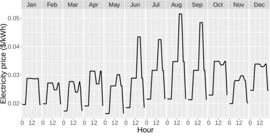
Jan Feb Mar Apr May Jun Jul Aug Sep Oct Nov Dec 0 12 0 12 0 12 0 12 0 12 0 12 0 12 0 12 0 12 0 12 0 12 0 12 0.02 0.03 0.04 0.05 Hour Electr icity pr ice ($/kWh)
Figure 2-2: Time-of-use charges that include energy and capacity costs.
In the case of RTP tariffs (RTP and RTP-Efficient), we calculate energy charges by replacing the flat tariff’s flat volumetric charge with our LMP prices from the PJM market in the U.S. Figure 2-3 shows the hourly average value for these charges.
Jan Feb Mar Apr May Jun Jul Aug Sep Oct Nov Dec
0 12 0 12 0 12 0 12 0 12 0 12 0 12 0 12 0 12 0 12 0 12 0 12 0.02 0.03 0.04 0.05 0.06 Hour Electr icity pr ice ($/kWh)
Figure 2-3: Real time pricing charges that include energy and capacity costs (hourly average).
As shown in table2.4, time-of-use and RTP tariffs also consider the flat volumetric charges to recover network and policy costs, as well as a fixed charge that recovers customer-specific cost streams. On the other hand, our RTP-Efficient tariff recovers all costs that are not associated to electricity generation, through fixed charges, equal for all customers.
In addition to several tariff designs, we consider three options for NEM schemes11: ∙ NEM "On": The first option, which we call NEM "On", consists on the strict application of NEM: Consumers are charged/paid the full volumetric retail tariff for consumption/exports of power to the grid.
∙ NEM "On-California": The second scenario mimics NEM schemes currently in force in California and Massachusetts in the U.S., where consumers are paid the full volumetric retail tariff, applicable to each time of the day, for grid exports that stem directly from solar generation or BTM storage that has been exclusively charged from solar panels (and not from the grid). Otherwise, their exports are valued at a lower rate, which in this work we assume to be equal to the energy charge of the tariff.
∙ NEM "Off": The third and last NEM regime considered is the NEM "Off" regime, where power consumption is priced at the full volumetric tariff but power exports are priced according to energy charges alone.
2.5
Solar generation modeling
In order to obtain a normalized solar generation profile applicable to the relevant jurisdiction, we use the same methods and data as (S. P. Burger, 2019).
In general terms, the model used to generate the profile is pvlib python, a Python-based tool developed by Sandia National Laboratories12.
The model uses solar irradiation and weather data, as well as PV system parame-ters such as efficiency, sizing of inverter, azimuth and other parameparame-ters. In this case, we use default parameters for a residential installation with 180∘ azimuth.13 14
11See section2.6for the mathematical implementation of these schemes. 12For a complete description of the model see (F. Holmgren et al.,2018).
13180∘ azimuth is the most common configuration among U.S. residential solar systems (Barbose
& Naïm,2019).
14Parameters are the same as used in (S. P. Burger,2019), i.e., System Type: Fixed Tilt; Tilt: 41.9;
DC-AC Derating: 1.3; Losses: 14% (system) and 4% (inverter); Temperature coefficient: -0.004; and Albedo: 0.2.
2.6
Storage operation modeling
In order to estimate how batteries would operate under the different tariff designs and NEM regimes, we develop a linear optimization model that is run for every customer that has been assigned a battery in our calculations.
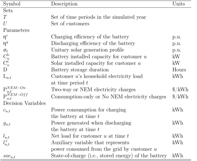
Table 2.5 shows the nomenclature used in the mathematical formulation of the model.
Symbol Description Units
Sets
𝑇 Set of time periods in the simulated year
𝑈 Set of customers
Parameters
η𝑐 Charging efficiency of the battery p.u.
η𝑔 Discharging efficiency of the battery p.u.
σ𝑡 Unitary solar generation profile p.u.
Cb𝑢 Battery installed capacity for customer 𝑢 kW
Cs𝑢 Solar installed capacity for customer 𝑢 kW
D Battery storage duration Hours
L𝑢,𝑡 Customer 𝑢’s household electricity load kWh
at time period 𝑡
P𝑁 𝐸𝑀 −𝑂𝑛𝑢,𝑡 Two-way or NEM electricity charges $/kWh
P𝑁 𝐸𝑀 −𝑂𝑓 𝑓𝑢,𝑡 Consumption-only or No NEM electricity charges $/kWh
Decision Variables
𝑐𝑢,𝑡 Power consumption for charging kWh
the battery at time 𝑡
𝑔𝑢,𝑡 Power generated when discharging kWh
the battery at time 𝑡
𝑙𝑢,𝑡 Net load for customer 𝑢 at time 𝑡 kWh
𝑙𝑢,𝑡+ Auxiliary variable that represents kWh
power consumed from the grid by customer 𝑢
𝑠𝑜𝑐𝑢,𝑡 State-of-charge (i.e., stored energy) of the battery kWh Table 2.5: Optimization model nomenclature.
2.6.1
Mathematical formulation for NEM "On" and NEM "Off"
regimes
The model minimizes the total bill paid by the customer, considering all volumetric charges under perfect foresight.15 Equation (2.1) is the objective function of the model (see table 2.5 for detailed nomenclature). It is important to clarify here that the term 𝑙𝑢,𝑡 represents the customer 𝑢’s net load, and is calculated by summing up the customer’s electricity consumption (L𝑢,𝑡) (e.g., household appliances), plus power consumed to charge the battery (𝑐𝑢,𝑡), minus the power output from the battery (𝑔𝑢,𝑡) and power output from installed solar PV panels (𝑠𝑢,𝑡) (see equation (2.2) for the mathematical formulation). The model is run separately and independently for each customer 𝑢 ∈ 𝑈 . min 𝑔𝑢,𝑡,𝑐𝑢,𝑡 ∑︁ 𝑡∈𝑇 (P𝑁 𝐸𝑀 −𝑂𝑛𝑢,𝑡 · 𝑙𝑢,𝑡+ P𝑁 𝐸𝑀 −𝑂𝑓 𝑓𝑢,𝑡 · max(0, 𝑙𝑢,𝑡)) (2.1) s.t.: 𝑙𝑢,𝑡 = L𝑢,𝑡− 𝑔𝑢,𝑡+ 𝑐𝑢,𝑡 − 𝑠𝑢,𝑡 ∀𝑡 ∈ 𝑇, (2.2)
The left-hand side of the objective function represents the minimization of the customer’s bill under the NEM "On" regime. That is to say, at any point in time 𝑡, both injections of power to the grid and consumption of power from the grid16,
are both valued at the same rate. Hence, when we run the model under a tariff design considering the NEM "On" case, all volumetric charges will be allocated in the P𝑁 𝐸𝑀 −𝑂𝑛𝑢,𝑡 term of the equation and the P𝑁 𝐸𝑀 −𝑂𝑓 𝑓𝑢,𝑡 term will be equal to 0 for all 𝑡.
In the case where there is no NEM scheme in force, we differentiate between two-way (or NEM-On) charges and consumption only (or NEM-Off) charges. Hence,
15Since we do not consider demand charges and fixed charges do not influence the operation of
customer’s DER portfolio.
16I.e., both negative and positive values of 𝑙
when we run the model under a tariff that does not include a NEM scheme, we will allocate charges that remunerate electricity generation (i.e., generated energy costs) in the P𝑁 𝐸𝑀 −𝑂𝑛𝑢,𝑡 term and all other volumetric charges17 in the P𝑁 𝐸𝑀 −𝑂𝑓 𝑓𝑢,𝑡 term. Consequently, injections of power to the grid on part of the consumer (negative values of 𝑙𝑢,𝑡), will be valued at P𝑁 𝐸𝑀 −𝑂𝑛𝑢,𝑡 , whereas consumption of power from the grid (positive values of 𝑙𝑢,𝑡), will be valued at P𝑁 𝐸𝑀 −𝑂𝑛𝑢,𝑡 + P
𝑁 𝐸𝑀 −𝑂𝑓 𝑓
𝑢,𝑡 .
In all NEM scenarios, the models work under the assumption that the operator of the battery is able to foresee all electricity charges with complete certainty throughout the simulated year (i.e., perfect foresight of charges). This constitutes an idealization of the real problem, where charges may change throughout the year (e.g., under real-time pricing). Since more realistic considerations would constrain the ability of the battery to optimize the customer’s consumption, what we estimate here is a lower bound of the bill that the storage owner would pay, if he/she could not foresee electricity charges with complete certainty.
Note that the optimization problem composed by equation (2.1), (2.2) and the subsequent constraints can be easily transformed to an equivalent linear optimization model by defining the auxiliary variable 𝑙𝑢,𝑡+; replacing the term max(0, 𝑙𝑢,𝑡) with 𝑙+𝑢,𝑡; and adding the following constraints:
𝑙+𝑢,𝑡 ≥ 𝑙𝑢,𝑡 ∀𝑡 ∈ 𝑇, (2.3)
𝑙+𝑢,𝑡 ≥ 0 ∀𝑡 ∈ 𝑇, (2.4)
The model also includes constraints that allow us to simulate in a simple way, the physical operation of batteries. For instance, equation (2.5) links the state of charge (𝑠𝑜𝑐𝑢,𝑡) of the battery in each time period with electricity generation and charging decisions. On the other hand, (2.6) sets the storage capacity limit for the battery equal to the maximum power output times the duration (i.e., the maximum amount of time that the battery can generate electricity at nominal output if fully charged),
while (2.7) and (2.8) set upper bounds of power output and input according to the assumed limits of the battery.
𝑠𝑜𝑐𝑢,𝑡 = 𝑠𝑜𝑐𝑢,𝑡−1− 𝑔𝑢,𝑡 η𝑔 + 𝑐𝑢,𝑡· η 𝑐 ∀𝑡 ∈ 𝑇, (2.5) 0 ≤ 𝑠𝑜𝑐𝑢,𝑡 ≤ Cb𝑢· D ∀𝑡 ∈ 𝑇, (2.6) 0 ≤ 𝑔𝑢,𝑡 ≤ Cb𝑢 ∀𝑡 ∈ 𝑇, (2.7) 0 ≤ 𝑐𝑢,𝑡 ≤ Cb𝑢 ∀𝑡 ∈ 𝑇, (2.8)
Additionally, solar generation for customer 𝑢 at time 𝑡, is given by the solar profile, which in our case is common for all users:
𝑠𝑢,𝑡 ≤ σ𝑡· Cs𝑢 ∀𝑡 ∈ 𝑇, (2.9)
2.6.2
Mathematical formulation for the NEM "On-California"
regime
We also model an additional NEM regime, which aims at modeling NEM schemes in force in California and Massachusetts, where storage can gain NEM credits only if the system is charged with power generated in consumer’s premises (exclusively solar in the case of California).
In order to model this NEM regime, we modify our model in order to allow for the storage system to charge exclusively from the solar generated power and not using power consumed from the grid.
Firstly, we remove the term 𝑐𝑢,𝑡 from equation (2.2), in order to avoid the model to consider an explicit monetary cost when charging the battery. Consequently, we replace equation (2.2) by (2.10):
𝑙𝑢,𝑡 = L𝑢,𝑡− 𝑔𝑢,𝑡− 𝑠𝑢,𝑡 ∀𝑡 ∈ 𝑇, (2.10)
Secondly, we replace equation (2.9) with the following:
𝑠𝑢,𝑡+ 𝑐𝑢,𝑡 ≤ σ𝑡· Cs𝑢 ∀𝑡 ∈ 𝑇. (2.11)
Consequently, solar available power (right hand side of constraint (2.11)) should be distributed among solar generation and storage charging power. This way we ensure that the battery charges only when there is solar power available and that total charging power is limited by total solar availability.
The rest of the set-up in this case is identical to the NEM "On" case described above.
2.6.3
Assumptions
Regarding batteries technical parameters, we base our assumptions in the most recent Lazard report (Lazard, 2019). Hence, we assume a 90% round-trip efficiency, with equal charging and discharging efficiencies. Moreover, we assume a 4-hour storage duration and an installed capacity equal to 60% that of the customer’s solar installed capacity.
Solar installed capacity is calculated for each customer separately, on the basis that the solar energy generated would offset 90% of the customer’s yearly load.18
The rest of parameters have been calculated as described in sections 2.4 for elec-tricity charges and section2.5 for the solar generation profile.