Dynamic pixel selection in free-space photon-counting optical communication systems for the exploitation of excess channel capacity

Dynamic Pixel Selection in Free-Space

Photon-Counting Optical Communication Systems

for the Exploitation of Excess Channel Capacity

by

Nivedita Chandrasekaran

S.B., Massachusetts Institute of Technology (2008)

Submitted to the Department of Electrical Engineering and Computer

Science

in partial fulfillment of the requirements for the degree of

Master of Engineering in the Department of Electrical Engineering

and Computer Science

at the

MASSACHUSETTS INSTITUTE OF TECHNOLOGY

June 2009

@ Massachusetts Institute of Technology 2009.

Author ...

All rights reserved.

MASSACHUSETTS INSTUTE OF TECHNOLOGY

JUL

2

0

2009

...

Department of Electrical Engineering and Computer Science

May 22, 2009

Certified

by...

MIT Lincoln Laboratory,

,-I

A,/

/

Pablo I. Hopman

Group 99Assistant Group Leader

I' / IV

Thesis Supervisor

Certified by...

...

/V

Jeffrey H. Shapiro

Julius A. Stratt

Professor of Eletrical Engineering

.. I

2

Accepted by

...

Arthur C. Smith

Chairman, Department Committee on Graduate Theses

ARCHNVES

Dynamic Pixel Selection in Free-Space Photon-Counting

Optical Communication Systems for the Exploitation of

Excess Channel Capacity

by

Nivedita Chandrasekaran

Submitted to the Department of Electrical Engineering and Computer Science on May 22, 2009, in partial fulfillment of the

requirements for the degree of

Master of Engineering in the Department of Electrical Engineering and Computer Science

Abstract

Atmospheric turbulence in free-space optical communications turns signal demodula-tion and decoding into a multimode problem as wavefronts of the transmitting laser beams are warped spatially past the desired form of a diffraction-limited spot at the receiver end of a free-space optical receiver. Adaptive optics, a traditional solution to this problem, is computationally expensive and adds complexity to receiver ar-chitecture by requiring tools like wavefront sensors and deformable mirrors. Due to the enabling technology of Geiger-mode avalanche photodiode (GM-APD) arrays, a simple algorithm that only requires information from the GM-APD array to imple-ment the technique of dynamic pixel selection can be realized entirely in software or firmware. Dynamic pixel selection exploits the temporal and spatial information attached to each received photon by filtering out noisy or otherwise undesirable por-tions of the array in order to exploit any excess channel capacity in the link to allow on-the-fly adjustments of data rates. Preliminary results, specific to the MIT Lin-coln Laboratory photon-counting, free-space optical communication system, which utilizes an 8 x 8 GM-APD receiver array, operates at a 1.06pm wavelength with 16-PPM signalling, and supports data rates up to 10 Mbps over 1-5km long paths, will be discussed.

Thesis Supervisor: Pablo I. Hopman

Title: MIT Lincoln Laboratory, Group 99 Assistant Group Leader Thesis Supervisor: Jeffrey H. Shapiro

Acknowledgments

I would like to thank my supervisor, Pablo Hopman, for all his guidance and support throughout my thesis. In particular, his questions about the point of the work I was doing helped me truly understand the basic theory that lay behind my thesis and what, exactly, performing good research entails. His constant push to have me explain my thought processes in layman's terms also helped me gain a complete understanding of my thesis work to the point where I could explain it to anyone regardless of their technical background.

Thank you to James Glettler for his detailed explanations that helped me com-pletely understand the actual Lincoln Lab communication system, despite the years of code that lay behind it. Thank you to Tom Karolayshn, Andrew Stimac, and Matt Hansen for their help in setting up the testbench for my experiments. In addition, I would like to thank to all the members of Group 99 for making my two years at MIT Lincoln Laboratory fun and productive.

I would also like to thank my on-campus thesis supervisor and academic advisor, Professor Jeffrey Shapiro, for his invaluable insights, questions, and thoroughness in making sure that I understood all of the background and theory that motivated my thesis. Without him, this thesis would not have achieved its current breadth and depth. Thanks to him, this thesis is a document that I can be proud of.

I would like to thank my parents for keeping me sane, offering sound life advice, and plying me with food and custom-roasted coffee beans through my years at MIT. Finally, thank you to all of my friends at MIT who helped make my M.Eng year at MIT one of the most entertaining and interesting years in my college career!

Contents

1 Introduction 17

1.1 Free-space optical communication systems . ... 17

1.2 The Lincoln Laboratory FSO photon-counting communication system 22

1.3 Organization of Thesis ... ... 24

2 The physics of free space optical communication 27

2.1 Signal propagation in a free-space optical communication link . . . . 29

2.1.1 Ideal propagation in an optical communication link ... 29

2.1.2 Propagation with thin-lens aberrations . ... 31

2.2 Accounting for atmospheric turbulence in a free-space optical

commu-nication system ... ... ... ... 32

2.2.1 The Greenwood frequency . ... . 33

2.2.2 The Fried parameter ... 33

2.3 Multimode reception in an optical communication link and the role of

Dynamic Pixel Selection ... ... .. 34

3 Selecting an Optimization Metric 41

3.1 Requirements for a metric ... 41

3.2 LLFSO System Operation - deriving signal and background power per

mask ... . ... ... 43

3.3 Defining the limiting factors in the system . ... 45

3.5 Evaluating the channel capacity of an idealized version of the LLFSO link ...

3.6 Evaluating the link margin of a 16-PPM Poisson channel as a metric

3.6.1 Versatility and Meaningfulness . ...

3.6.2 Parametrizability over over ns, nb, and M -Monte-Carlo

meth-ods and LUT Generation . ...

3.6.3 Optimizability ...

4 Dynamic pixel selection

4.1 The POISSON-FIT block . . ...

4.1.1 Retrieving temporal photon count information . .

4.1.2 Calculating nsi and nbi . . ...

4.1.3 The Poisson Maximum Likelihood Estimator and

Error... 4.2 SORT block ...

4.2.1 The sorting metric ...

4.2.2 Sorting by psi . ...

4.3 METRIC block ...

4.4 Conclusion ...

5 Performance analysis of the

5.1 The testbench system and

5.2 Selecting testing points . . 5.3 Discussing data sets .. .

55 57 57 58 Estimation . . . 60 DPS algorithm 71 decoder . ... 72 .. . . . . . . . . 74 .. . . . . . . . 78

5.3.1 Test Point 1: Plateau region, n, > M * rib, ns = 6.5, nb = 0.1 .

5.3.2 Test Point 2: Non-plateau region, n, > M* nb, ns = 2.3, nb = 0.1 5.3.3 Test Point 3: n, M ri b, ns = 4.4, nb = 0.3 ...

5.3.4 Test Point 4: Non-plateau region, n, < M * nb, n, - 4.0,

nb = 0.511 ...

5.3.5 Test Point 5: Plateau region,ns < M * nb, ns = 5.9, nb = 0.5

5.4 Analysis and conclusions ...

6 Conclusions and Findings 97

A Numerical calculation of the capacity of a 16-PPM Poisson channel

using Monte Carlo Methods 99

B Project Code 105

List of Figures

1-1 An example of a possible network constructed out of air-to-air,

ground-to-air, and ground-to-ground free-space optical communication links.. 18

1-2 The electromagnetic spectrum, adapted from [14]. . ... . . 19

1-3 A sketch of the field of views of the transmitter and receiver of a

free-space optical communication link. . ... . 20

1-4 The end-to-end testbench implementation of the Lincoln Laboratory

FSO communication system. Modified from [13] ... 23

2-1 Geometry of point-source illumination of a plane screen Fresnel-Kirchoff diffraction formula. Modified from Fourier Optics by Joseph W.

Good-man. . ... ... ... 29

2-2 Geometry for calculating the Greenwood frequency fG and the Fried parameter ro. Modified from Principles of Adaptive Optics by Robert

K. Tyson. .... .. ... . ... ... 34

2-3 Focusing optics in an optical receiver. An incoming plane wave from an

ideal propagation path is transformed into an Airy function. Derived

in part from [7]... 35

2-4 Geometry for determining the number of spatial modes an optical re-ceiver detects. The orthogonal frequency components of the incoming plane waves are imaged into orthogonal spatial components at the

im-age plane. Derived in part from [7]. ... .. ... . 35

2-5 Comparing long-exposure point-spread functions to an expected

2-6 A sketch of the areas over which a multimode detector would receive

power under poor and good seeing conditions. . ... . 38

3-1 Minimum signal power required to successfully decode at a given back-ground power for the implemented system, for a system with losses due to the SCCC turbodecoder alone, and for the ideal system capable of

achieving Shannon capacity. ... .... 46

3-2 General block diagram of a communication system. Modified from

Elements of Information Theory by Cover and Thomas... 48

3-3 3D and contour plots of the capacity of a 16-PPM Poisson channel. . 53

4-1 The DPS algorithm is placed between the GM-APD detector and the

Receiver system in order to filter photon data sent to the Decoder... 55

4-2 General block diagram of the Dynamic Pixel Selection algorithm. . 56

4-3 Receiver time synchronization -SYNC tones add coherently, while data

symbols and noise add incoherently. Modified from 'An End-to-End Demonstration of a Receiver Array Based Free-Space Photon Counting

Communications Link' by P. Hopman and L. Candell. . ... 58

4-4 Calculating n, from raw photon count data given Q = 1, tlot = 12.9ns.

Both the temporal and spatial locations of the photons are used to

calculate the ni, or the number of signal photons per ith pixel per

time slot over the entire GM-APD array. . ... 59

4-5 A given raw array of ni and nbi over an 8 x 8 GM-APD array for

Q

SORT block generates when selecting the top 1, 9, 18, and 64 pixels. . 64

4-6 A plot of the way n, and nb for Q = 1 and tso1 t = 12.9ns increase over

the generated masks as the number of top pixels selected in a given spatial mask is increased. The raw data used to generate these plots

was also used to generate Figure 4-5. . ... . . 65

4-7 The functional block diagram detailing the operation of the METRIC

4-8 An example data rate optimization of the METRIC block in units of

bits

second...

5-1 A bird's eye view of the receiver end of the LLFSO testbench system. 5-2 Graphical User Interface output when testbench system receiver is

suc-cessfully receiving and decoding payload data . ...

5-3 Contour plots of the gradient of the Shannon capacity in bits with respect to changes in signal and background strengths. In addition, lines corresponding to n, = 16nb are plotted to show the point at which signal and background strengths are equal in a received 16-PPM symbol. 5-4 The 5 test points in (ns (signal photons per slot),nb (background

pho-tons per slot)) that will be employed to validate the DPs algorithm across the full range of operating conditions. The plots are referenced

against DapatY n,n threshold signal strength nsmi(nb), and line along

which the signal and background strengths are equal over a single symbol. 5-5 DPS capacity 5-6 5-7 5-8 5-9 5-10 5-11 5-12 5-13 5-14 DPS DPS DPS DPS DPS DPS DPS DPS DPS capacity capacity capacity capacity capacity capacity capacity capacity capacity margin margin margin margin margin margin margin margin margin margin

optimization with spatial masks in Test Point 1. and signal margin

optimization with and signal margin optimization with and signal margin optimization with and signal margin optimization with and signal margin

optimization in Test Point 1. spatial masks in Test Point 2. optimization in Test Point 2. spatial masks in Test Point 3. optimization in Test Point 3. spatial masks in Test Point 4. optimization in Test Point 4. spatial masks in Test Point 5. optimization in Test Point 5.

5-15 SCCC decoder iterations as a function of M ap, sig . . . . .

A-1 A graphical representation of the typical set and atypical set of an

n-long sequence drawn from a distribution p(X) . . . . .

A-2 Entropy of a Poisson random variable versus the rate parameter A. A-3 logo contour plot of number of required iterations versus n, and nb.

95

100 102 103

List of Tables

3.1 Q factors and data rates for a system with to1 t = 12.9ns, M = 16, and

r ... ... 44

3.2 nsmin(nb) ... ... 45

5.1 DPS Algorithm operation in Test Point 1 . ... 81

5.2 DPS Algorithm operation in Test Point 2 . ... 82

5.3 DPS Algorithm operation in Test Point 3 . ... 87

5.4 DPS Algorithm operation in Test Point 4 . ... 90

Chapter 1

Introduction

1.1

Free-space optical communication systems

Prior to the development and deployment of long haul fiber-optic communication systems, a network of line-of-sight microwave links served as the backbone for the telephone network. That network has now been supplanted by the fiber-optic com-munication infrastructure which has enabled the Internet age. There are, however, many situations in which the broadband capability provided by communication at optical wavelengths is desired, but in which it is inconvenient, unaffordable, or im-possible to establish a fiber connection between the desired endpoints. In this realm, free-space optical (FSO) communications are becoming the systems of choice.

The objective of a free-space optical communication system is to transmit infor-mation from one point to another via the use of mid-infrared to mid-ultraviolet carrier waves along a line of sight path between two points. The advantages of FSO com-munications are numerous [16] due to the fact that minimal infrastructure is required to construct these links. A network of terrestrial free-space links could be used to network an entire city together. The portability of free-space communication systems also lends them for use in temporary network installations that can also be used to re-establish communication links in the case of an emergency. The wavelength A of the carrier wave is a key parameter that is used to define two design drivers of a communication system [1]:

Figure 1-1: An example of a possible network constructed out of air-to-air, ground-to-air, and ground-to-ground free-space optical communication links.

* The beamwidth is defined as the divergence angle of an electromagnetic beam between its half-power points as it travels along its free space path. In the best

case, when the system is diffraction limited, the beamwidth is 2, where D is

the diameter of the transmitter aperture.

* The bandwidth is the span of frequencies used to carry information by the communication system. Generally speaking, for a system with carrier frequency

f

=

increas-ingly difficult as the communication bandwidth becomes an increasing fraction of f. Maximizing the communication bandwidth is desirable because it mini-mizes the time required to transmit a fixed-size message.

Radio and television stations broadcast their programs using radio waves waves with wavelengths ranging from 1 - 102 meters. Current satellite uplinks operate at in the Ka-band and X-band regions of the spectrum, which have wavelengths ranging from 1-10 centimeters. It is clear that the beamwidth and bandwidth design drivers both improve as the communications system uses electromagnetic waves with shorter and shorter wavelengths. Free-space optical communication systems that operate in the mid-ultraviolet to mid-infrared range of the spectrum, with wavelengths from 0.1 to 10 microns, thus offer orders of magnitude in improvements to the system's

Beamwidth

Bandwidth increases

Figure 1-2: The electromagnetic spectrum, adapted from [14].

beamwidth and bandwidth, as seen in Figure 1-2.

The narrower beamwidth of FSO enables the following system improvements

[16],[7],[1].

* The narrower beam conveys greater signal power per steradian. As a result, op-tical transmitter and receiver components can be smaller, lighter, and consume less power than their radio-frequency counterparts.

* FSO communication links do not operate in the 3kHz-300GHz frequency

spec-trum that is regulated by the Federal Communications Commission (FCC). As a result, they do not require FCC licensing or frequency allocation.

It is clear that a typical free-space optical communication link like the one seen in Figure 1-1 has significant advantages over lower-frequency communications. However, the same short wavelength and high carrier frequency lead to significant limitations on FSO communications.

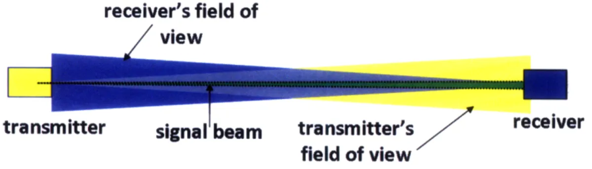
The first major limitation of any free-space link is the requirement of an unob-structed line-of-sight path between the transmitter and receiver in order for informa-tion to be transmitted. In addiinforma-tion, the transmitter and receiver must also be pointed such that their fields of view intersect one another as shown in Figure 1-3. Indeed, the

receiver's field of

view

transmitter

signal beam

transmitter's

receiver

field of view

Figure 1-3: A sketch of the field of views of the transmitter and receiver of a free-space optical communication link.

narrow beamwidths of FSO communications make establishing and maintaining the alignment shown in Figure 1-3 a much more significant challenge than the comparable problem in the radio-frequency region. This thesis does not address the challenges of pointing in a free-space optical communication system.

The second major limitation of a free-space optical link arises when the propaga-tion path lies partly or wholly within the earth's atmosphere. The presence of clouds, fog, rain, or snow in the propagation path of an FSO link will severely to

catastroph-ically degrade its communication performance owing to the pronounced scattering

-and at some wavelengths, absorption - of the optical beam. Consequently, the

desir-able narrow-beam high data rate operating regime for atmospheric-path FSO systems is limited to clear-weather conditions. However, even in clear weather, an FSO link must contend with the effects of atmospheric turbulence.

Atmospheric turbulence refers to the random changes in the refractive index of the atmosphere caused by turbulent mixing of air parcels with approximately 1 Kelvin temperature differences. Turbulence degrades FSO links in a variety of ways. The transmitter beam can be spread by turbulence to a divergence beyond the beamwidth predicted by diffraction theory, which in turn causes a decrease in the signal power collected at the receiver. There can also be beam wander, or the random motion of the centroid of the signal-power spot in time at the receiver. Turbulence also causes angular spread. For example, instead of all the light arriving arriving at the receiver along the diffraction-limited line-of-sight path, a broader range of arrival angles can occur, thus blurring the signal-power spot seen in the focal plane of a

receiving telescope. Worst of all, turbulence causes fading, known as scintillation, that can bury the communication signal in atmospheric background light. Improving the performance of an FSO link operating in the presence of atmospheric turbulence is the ultimate goal of this thesis.

In order for an FSO communication system to successfully convey information, sufficient signal power must be detected at the receiver to overcome any accompany-ing noise. As a result, an optical receiver in a free-space communication link must have an aperture sized to compensate for turbulence-induced beam spread and beam wandering. Similarly, the receiver field of view must be sufficient to accommodate any turbulence-induced angular spread. Increasing the receiver aperture and its field of view also increases the amount of background light that it collects. Furthermore, the increased field of view will require the use of a larger photodetector or photodetector array. In general, this larger detector size leads to increased detector noise, like an increased dark current. For convenience in what follows, all of the preceding noises will be lumped together and referred to collectively as background noise.

Background noise is thus a key limiting factor for free-space optical communication systems and is one this thesis will address. In particular, we will be interesting in optimizing signal power collection while minimizing background power collection so as to get the best overall communication performance.

Given an optical communication link, the signaling scheme, and the model for the noise added to the channel over which the information is transmitted, a metric referred to as the 'Shannon channel capacity,' or simply the 'channel capacity', can be derived. Only the signaling scheme, amount of signal power, and amount of back-ground power present in received symbol affect the value of this metric. Shannon's channel capacity theorem is extremely useful and provides an operational definition for this metric. Shannon's theorem states that for any data rate less than the channel capacity, there exists an encoding and decoding scheme such that received codewords can be decoded with an arbitrarily small bit error rate. For data rates above the channel capacity, reliable information transmission is impossible. It is easy to see that FSO channel capacity increases with increasing signal power and decreases with

increasing background power at the receiver. Thus, it is immediately apparent that there is a very definite advantage in being able to selectively increase signal power while rejecting as much noise as possible.

In this thesis, we will derive, design, and test a data-rate optimization algorithm that selectively maximizes signal power collection while minimizing background noise on the MIT Lincoln Laboratory FSO communication system in order to increase the data rate at which the link operates.

1.2

The Lincoln Laboratory FSO photon-counting

communication system

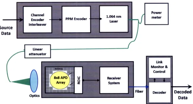
The MIT Lincoln Laboratory FSO Communication System (LLFSO) is a photon-counting communication system intended for use in clear-weather conditions over terrestrial links ranging from 1 to 5 kilometers in length. These terrestrial links can either be ground-to-ground or air-to-ground. In the LLFSO, source data is converted into a bit stream, which is then encoded into optical pulses for transmission. The receiver detects the light pulses and decodes them back into data. While a full implementation of the ground-to-air link does exist, the development and testing of Dynamic Pixel Selection, the algorithm developed in this thesis, took place on an end-to-end testbench implementation of this system. The block diagram of the components of the testbench is shown in Figure 1-4.

A detailed description is available in [13]. For our purposes, the following char-acteristics are germane. Data is encoded in a 16 Pulse Position Modulation (PPM) format such that a single photon occupies one of 16 time slots in a transmitted sym-bol. Thus, each signal photon can encode up to 4 bits of information. However, background noise in the link can easily corrupt the 16-PPM symbols such that the receiver may decode one or more of the transmitted symbols incorrectly. As a result, the link uses a rate-! Serially Concatenated Convolutional code (SCCC) that allows the link to operate within 1 dB of the Shannon capacity of the link [21].

Source Data

pticsDecoder _Opts Decoded

Data

Figure 1-4: The end-to-end testbench implementation of the Lincoln Laboratory FSO communication system. Modified from [13].

This efficient signaling scheme is constructed around the assumption that single photons can be detected with a narrow timing resolution on the order of nanoseconds. The technology that has enabled this assumption is the fabrication of arrays of Geiger Mode Avalanche Photodiode (GM-APDs). The GM-APDs used in the LLFSO de-tector have been designed for use in a laser-communication system transmitting at near-infrared wavelengths. LLFSO GM-APDs have photon detection efficiencies of up to 50% and dark count rates of less than 20 kHz [24]. They are highly reverse-biased diodes that switch from high-impedance to a low-impedance devices when an initial photon absorption in the diode junction causes an avalanche of additional charge carriers who presence is easily detected in the external circuit. While this extreme sensitivity to impinging photons is what makes the GM-APD such an excellent pho-ton detector it is also the cause of the unique challenges faced by a receiver using GM-APDs.

The first unique challenge is detector holdoff time. After an avalanche has been triggered, the GM-APD can only be re-armed once sufficient time has passed to ensure that all additional photocarriers have streamed through the diode junction. This holdoff time requirement means that after one photon has been detected, the

GM-APD will be blind to any signal photons that arrive during the holdoff period. The LLFSO compensates for this possible blocking loss of signal photons by using an 8 x 8 array of GM-APDs. The receiver optics distribute the incoming photon flux over several detectors in the array, reducing the flux incident on a single detector and hence decreasing the likelihood that blocking loss will occur. An additional consequence of this approach is the fact that the Poisson statistics of photons incident on the array are preserved due to the absence of blocking loss effects [8].

The use of a GM-APD array, as just described, entails an additional tradeoff. Each detector added in the array contributes its own dark counts and collected background light. Thus, the specific system components of the LLFSO also motivate the need for a spatial filter that could be dynamically resized to fit to a signal spot spread out over the array.

The LLFSO system is capable of data rates up to 10 Mbps with communication efficiencies of greater than 1 bit per photon. However, its use of GM-APD arrays as well as the nature of any general free-space optical communication link motivates the need for the Dynamic Pixel Selection (DPS) algorithm that will be the focus of this thesis.

1.3

Organization of Thesis

The goal of the Dynamic Pixel Selection algorithm is to turn GM-APD detectors in the 8x8 GM-APD array on and off in order to compensate for atmospheric turbulence and improve the performance of the system. The following chapters first set up the problem of optimizing the

Chapter 2 deals with the problem of what the signal beam arriving at the GM-APD looks like after it has propagated through atmospheric turbulence. Chapter 2 presents the atmospheric and optical physics necessary to motivate and quantify the characteristics of the received signal to emphasize the need for the Dynamic Pixel Selection algorithm. In addition, the two parameters that define the bandwidth and resolution of the algorithm will be determined. The question of how the receiver

ex-tracts the field-of-view information from the frequency content of the received optical signal will be answered. In order to make the previous listed tasks tractable, the Kolmogorov long-exposure model for atmospheric turbulence will be assumed.

Chapter 3 then discusses how the algorithm should rate the different masks that will be used to filter incoming photon data from the GM-APD. In order to do this, the performance of a communication link is be measured and predicted given signal and background photon counts at the receiver end of the link using the link's channel capacity so that each of the masks can be linked to a number defining the overall performance of the link.

Chapter 4 discusses the overall function of the DPS algorithm the algorithm raises the data rate and improves the bit error rate of the LLFSO communication system. In order to do this, the chapter traces through the entire algorithm, function block by function block. The assumptions made in the design of each block, inputs to each block, and the function of each block are discussed.

Chapter 5 presents the data used to test the DPS algorithm in all of its possible operational modes. First, the testbench setup is discussed, as are the methods used to characterize a real, implemented, and imperfect system. Then, the the number and value of the test points needed to induce all possible modes of the DPS algorithm are derived and discussed. Finally, results from the test points are presented.

Chapter 2

The physics of free space optical

communication

High data-rate FSO communication over an atmospheric path is only possible in clear weather. Even then, there are significant complications that would not be present were the link established through optical fiber. In particular, the FSO link must overcome three major problems if it is to transmit information reliably:

* The transmitter must be stably pointed onto the line-of-sight propagation path to the receiver, and that receiver must include the transmitter in its field of view.

* The system must employ means to compensate for link dropouts caused by turbulence-induced fading.

* The link must be arranged to handle the time-varying beam spread and angular spread arising from atmospheric turbulence.

This thesis assumes that the problem of stable pointing has already been solved for the LLFSO system. In addition, it assumes that fading due to turbulence can be handled by the second-long interleaving time included in the source data encoding. The focus here will thus be on compensating for the beam spread and beam wander effects in the received optical signal. The multidimensional problem of accounting

for the temporal and spatial transformations of the transmitted optical signal at the detector plane must therefore be understood in order to proceed.

In order to successfully extract the maximum amount of signal power from the received data while rejecting a a maximum amount of background power, a free-space optical communication receiver must either have an aperture small enough to select a single mode of the received signal, or must be capable of treating the problem of signal extraction as a multimodal problem. Small apertures are limited by the fact that usually admit low amounts of widely spread signal beams and may not allow enough signal power through to the decoder for the link to operate reliably. As a result, the multimodal receiver solution is greatly preferable.

Section 2.1 frames the problem of imaging with aberrations in a tractable way by making the appropriate assumptions about the wave equations of the propagating beam and the system functions of the atmosphere. It presents the optical physics necessary to derive the way in which the optical signal propagating along a free-space path transforms before it is detected at the receiver.

Section 2.2 defines two parameters that are used to define the type of atmospheric turbulence, known as the long-exposure Kolmogorov turbulence model, for which the LLFSO-specific DPS algorithm can compensate in real-time without encountering la-tency constraints. The two parameters are the Fried radius, which is used to quantify the beam spread in a FSO system due to atmospheric seeing, and the Greenwood frequency, which specifies the time scale for temporal changes in turbulence.

Section 2.3 combines the derivations for laser propagation in Section 2.1 with the spatial parameters derived in Section 2.2 in order to discuss the need for the DPS algorithm.

2.1

Signal propagation in a free-space optical

com-munication link

2.1.1

Ideal propagation in an optical communication link

In order to formulate a tractable method of dealing with a transmission signal as it propagates in a free-space link, the spatial content of the source will be taken to be a complex envelope U(z), which we will assume to be a coherent spherical wave that diffracts through a circular transmitter aperture. Neglecting diffraction for now, U(z) satisfies

ejkz

U(z) =

where k = 2 is the wave number, and z is the distance from the source point.

Following Tyson's derivation [23], a coordinate system is constructed in which the

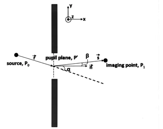
Kirchoff integration rule can be applied to the spherical wave equation along the area of the aperture. The source is located at the point Po in the (xo, Yo) plane and is a

I pu I lpan, P P S

source, PO _{imaging point, P1}

Figure 2-1: Geometry of point-source illumination of a plane screen Fresnel-Kirchoff diffraction formula. Modified from Fourier Optics by Joseph W. Goodman.

distance z0o from the pupil plane. The point at which the wave is measured, P1, is

located at (XI, yi) and is a distance zl away from the pupil plane. The pupil plane, P' is defined to be located in the (x', y') plane. The field at Pi is given by a 2D surface integral over the aperture AP that can be written in rectangular coordinates [10] as follows:

U(xI) A jk(r+ls) (cos/ - cos a)dS (2.2)

U(y)-2j

I

For typical FSO systems the assumption of far-field propagation can then be made, i.e.

k(x'2

+ y'2)max

z 2 (2.3)

which collapses (2.2) into the Fraunhofer diffraction integral,

U(xj, yx) = jzl) I_ A U (x ' y _{C 2) ' (}x_lx _{+Yly)dx'dy' (2.4)}

oc F[U(x', y')] (2.5)

where Y denotes the spatial Fourier transform evaluated at the spatial frequencies

fx

With this framework in place, the width of a diffraction-limited coherent spherical wave in the far field can be easily evaluated. Specifically, we get the following closed form equation for the intensity when the aperture is circular with a diameter R, as seen in [10]

()

(r) = 2 Az (2.6)

jzA 2xrRr

Here the intensity is expressed in cylindrical coordinates where r2 = x2 + y2. A = R27r is the area of the diffraction pupil; and Jl(x) is a first-order Bessel function. This intensity distribution is known as the Airy pattern.

This closed form for the intensity of a coherent beam in the best-case scenario of a diffraction-limited FSO system offers a lower bound for the beam spread of a source propagating through a medium with no aberrations. The distance d between the first

nulls of the Airy function provides that bound. It is given by zA

d = 2.44 (2.7)

D

providing the basic estimate for the beam spread of a diffraction-limited optical signal, which was discussed in Section 1.1. We will use this expression in Section 2.3 when the problem of refocusing the received optical signal is discussed. It will also be used to define the solid angle required for the detector to collect approximately 84% of the signal power.

2.1.2

Propagation with thin-lens aberrations

Now, a model for aberrations along the free-space propagation path will be introduced. This model will preserve the idea that the far-field behavior is proportional to the spatial Fourier transform at the pupil plane.

To accomplish this we model all aberrations as thin lenses spread out along the propagation path. From Roggeman [17], the lens transmission function is given in cylindrical coordinates as

T(r = e- 2f (2.8)

where f is its focal length. The Fraunhofer equation at P1 then becomes

ejkzle zl ( 1 1Y ) f

U(xl,yl) = z

J

-k I)(x- x +Y1Y )dx'dy' (2.9)

After rescaling the coordinates of the integral in (2.9), it is seen that the spatial

frequencies of the new Fourier transform are now fx = x and

f,

1 = - --. Therefore, the cumulative effects of propagation and aberration along

a free-space path on the image of an object can be viewed as a series of Fourier transforms.

-(Up ₎ oc Y(Upa).T(PSF) (2.10)

where 0 denotes convolution. In (2.11), it is seen that the series of Fourier transforms modeling aberrations along the path can be combined into an imaging function known as the point spread function (PSF). PSFs will be used in Section 2.2 to create a simple function to model the very complicated aberrations of atmospheric turbulence.

2.2

Accounting for atmospheric turbulence in a

free-space optical communication system

Owing to approximately 1 Kelvin temperature variations in the atmosphere, it can be divided into pockets of air, call turbules, on the order of centimeters to meters in diameter that have indices of refraction differing in a few parts in a million. Warm air is less dense and has a lower index of refraction, while cold air is more dense and has a higher index of refraction. The denser, cold air sinks while the warm air rises. The mixing that occurs in this motion leads to atmospheric turbulence [22].

These turbules can be modeled as lenses with varying diameters and focal lengths. As they rise and fall due to temperature variations, they refract and blur optical sig-nals passing through them. Formulating a basic model of the atmosphere will allow a discussion of the parameter that defines the size of the spatial mode of a received op-tical signal that has propagated through the atmosphere, as well as the time constant that quantifies the time scale of atmospheric evolution. From these two parameters, as well as the thin lens approximation, point spread functions that provide a first-order approximation for the distribution of signal energy in the receiver's focal plane can be constructed.

Following the derivation in [2], we first assume that the turbulence is statistically homogeneous and isotropic so that its statistics do not depend on the choice of coor-dinate axes. In addition, dynamic pixel selection should be performed on time scales that are long compared to the correlation time of turbulence induced propagation effects. This approximation is called the long-exposure limit. Toward that end, we will use the Kolmogorov-spectrum turbulence model to quantify the time scale at

which the long-exposure approximation becomes valid.

2.2.1

The Greenwood frequency

The bandwidth at which an adaptive optics receiver should operate in order to com-pletely compensate for turbulence is the Greenwood frequency. This frequency is found from the frozen-flow hypothesis, which states that the turbules do not evolve as they blow across the transmission path [11]. For Kolmogorov-spectrum turbulence, the Greenwood frequency is given by

52

fG = 2.31A-5 secY C, (z)Vnd(z)dz (2.12)

where r is the propagation distance, C2(z) is the turbulence strength parameter along

the propagation path, and vwind is the transverse wind speed along that path. Typical

models for C (z) _{include the Hufnagel-Valley Boundary model, the SLC-Day model,}

or the Clear-1 Night model. These models are statistically constructed from data at

observed at varying locations [19]. Typical values for C2(z) range from 1 0-1m3 to

10-16m [22].

Over time scales that are short compared to -, the focal-plane spatial pattern in an FSO communication receiver will be frozen. The dynamic pixel selection algorithm, however, will be designed to work in the long-exposure limit when the receiver's focal-plane spatial pattern has been blurred by averaging over a time scale that is long

compared to I. Typical values of the Greenwood frequency range from 10-100 Hz

[11]. Thus the DPS algorithm should perform its updates on times scales at least an order of magnitude longer than 0.01-0.1 seconds.

2.2.2

The Fried parameter

The Fried seeing cell parameter ro can be thought of as the diameter of a thin lens that provides a first-order approximation to the long-exposure blurring, or angular spread, encountered at an FSO receiver. For the geometry in Figure 2-2, Fried found

altitude, z

/ propagation

zenith angle, path length,

- L=IVI

Figure 2-2: Geometry for calculating the Greenwood frequency fG and the Fried

parameter ro. Modified from Principles of Adaptive Optics by Robert K. Tyson.

that [6].

ro = 0.423k2 _{sec 0J C(z)dz}

(2.13)

Typical values for ro range from 4 to 20 mm. A beam received after propagation through atmospheric turbulence with a Fried parameter ro will have an angular spread

of _ro A instead of the diffraction limited value of _R , where R is the radius of the

receiver's aperture. Variations of ro, which occur on time scales much longer than '

change the size of the signal spot in the receiver's focal plane and motivate our DPS algorithm for dynamically restricted the receiver's field of view.

2.3

Multimode reception in an optical

communi-cation link and the role of Dynamic Pixel

Se-lection

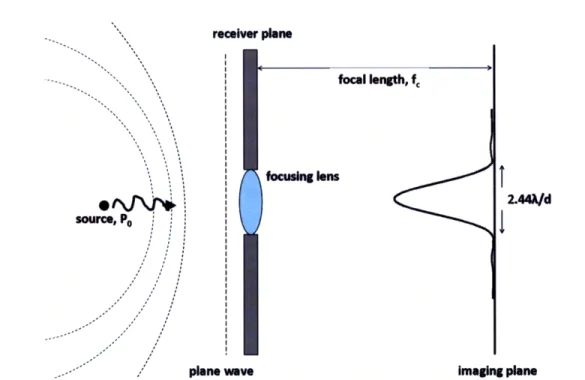
Figure 2-3 shows the propagation behavior for the ideal situation in which there is no turbulence. A point source propagates into the Fraunhofer regime so that a plane wave arrives at the receiver's entrance aperture. The received plane wave, which contains the 16-PPM temporal signal, contains no spatial information. From (2.8) we can show that the lens in Figure 2-3 will transform the received plane wave into the expected Airy pattern on the receiver focal plane where the GM-APD array will be located, as shown in 2-3 and written in (2.6).

source, P0 focal length, _f, roh\lo / / , /1 /i SI I Ile lt 2.44A/d imaging plane

Figure 2-3: Focusing optics in an optical receiver. An incoming plane wave from an ideal propagation path is transformed into an Airy function. Derived in part from

[7].

recever plane

focal length, f_c

n . 2.4d

plane Wave Imaging plane

Figure 2-4: Geometry for determining the number of spatial modes an optical re-ceiver detects. The orthogonal frequency components of the incoming plane waves are imaged into orthogonal spatial components at the image plane. Derived in part from [7].

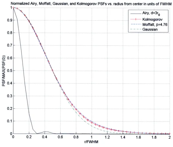
A single point source, in the absence of turbulence, becomes focused into an Airy function by the receiver lens. Thus, at best, any optical source can only be fo-cused to a diffraction-limited spatial resolution given by (2.7). A diffraction-limited optical system does not account for atmospheric turbulence. The long-exposure Kol-mogorov assumption makes it easy to calculate a point spread function that will account for angular spread arising from atmospheric turbulence. The Kolmogorov

Normalized Airy, Moffatt, Gaussian, and Kolmogorov PSFs vs. radius from center in units of FWHM

1-*

Figure 2-5: Comparing long-exposure point-spread functions to an expected

diffraction-limited Airy function with d=3ro.

point spread function, as given by (2.15), requires a Fourier transform calculation. Two simpler, closed-form expressions that closely approximate the general shape of the long-exposure Kolmogorov PSF are the Moffatt and Gaussian functions, given by

(2.16) and (2.17), respectively [12].

1

41n2

Note that the propagation effects enter these point spread functions only through the full-width half-maximum (FWHM) point of the beam, which is size for seeing by

setting FWHM = - where ro is the Fried parameter. With these results in hand

we can address the question of how large a field of view a detector requires in order to collect the majority of the energy from the received signal.

As shown in Figure 2-4, the solid angle occupied by light from a single point source when it is focused onto the detector plane is

Qmode-noatmosphere -- (2.18)

for a circular receiver aperture of diameter D when there is no turbulence and the propagation is diffraction limited. With atmospheric turbulence whose Fried seeing parameter is ro, a point source is transformed by the Kolmogorov long-exposure optical transfer function with an angular spread A. This beam passes through the focusing lens at the receiver plane. To a first order, this system can be modeled as two lenses in series with diameters ro and D. In this case, the actual solid angle covered by a point source at the imaging plane after it travels through a long-exposure model of the atmosphere with a seeing parameter ro and a focusing lens of diameter D is

Qmode = - + (2.19)

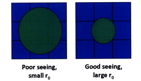
A smaller ro value corresponds to a signal intensity profile with a larger full-width half maximum (FWHM) point. Therefore, a smaller ro corresponds to worse seeing

conditions. The smaller ro is, the more diffuse the single signal mode that arrives at the detector is, as shown in Figure 2-6.

Poor seeing,

Good seeing,

small ro

_{large ro}

Figure 2-6: A sketch of the areas power under poor and good seeing

over which a multimode detector would receive conditions.

The detector's field of view, in steradians, when the overall array has a circular diameter d and the receiver lens has a focal length f, is

(2.20)

det = )2

4

fe

For a non-circular detector, Qdet is simply proportional to (A). The number of

spatial modes that can be contained within this field of view is found by dividing Qdet from (2.20) by the diffraction-limited field of view from (2.19)

Qdet Number of detected diffraction-limited modes =d

Qmode-noatmosphere

(dD

'AfcJ

(2.21) (2.22)

which we will assume to be greater than one. Because of turbulence, however, the number of diffraction-limited spots contained in a detector sized for the seeing

pa-rameter ro is

Qmode

Diffraction-limited modes in ro-sized detector = mode (2.23)

Qmode-noatmosphere

= )2 (2.24)

where ro is much smaller than D.

It is now easy to see why dynamic pixel selection will be valuable. Suppose that ro = 4 mm, as seen in [6] for a terrestrial path, and D = 127 cm. A diffraction-limited detector, with d d A, will collect only a signal mode of the signal beam's detector-plane spatial pattern. However, the spatial pattern is comprised of 105 modes. Hence the diffraction-limited receiver will suffer 50 dB of signal power loss when compared to a detector whose size is matched to the signal beam's focal plane pattern. By enlarging the detector, however, a much larger amount of background light is also collected. Dynamic pixel selection allows the receiver to optimize its performance for the prevailing ro value.

Given a multimode detector in the form of an 8 x 8 array of GM-APDs with pixels that can be dynamically turned off and on in order to select and pass on signal modes from receiver to decoder, an algorithm that uses this functionality to maximize the overall data rate of the system can be constructed. This algorithm is the Dynamic Pixel Selection algorithm. Its design and operation will be further discussed in Chapters 4 and 5. Before turning to that development, it will be valuable to establish the performance metric with which the DPS algorithm's behavior will be optimized.

Chapter 3

Selecting an Optimization Metric

Chapters 1 and 2 have made it clear that the Dynamic Pixel Selection algorithm will weigh different spatial filtration configurations of the GM-APD array with some sort of metric in order to choose the spatial filter that best maximizes the data rate and performance of the link. The discussion in this chapter, when contrasted with the mechanics of the algorithm in Chapter 4, will show that the complexity of the algorithm does not lie in its implementation but rather in the selection of the appropriate optimization metric for the DPS algorithm should. Metric selection will therefore be the task of this chapter.

After discussing the requirements for this optimization metric, we will define the signal and background photon fluxes over possible spatial masks. Next, peculiarities in the way the data rate is changed in the LLFSO will be discussed in order to quantify how the data rate changes affect the signal and background photon fluxes. Finally, two possible metrics, the link signal margin and the link data-rate margin will be discussed. Finally, the link data-rate margin will be selected as the appropriate optimization metric.

3.1

Requirements for a metric

The LLFSO receiver performs soft-decision iterative decoding of incoming 16-PPM signals by evolving the log-likelihood ratios attached to the incoming data in order

to select the most probable symbol. This is in contrast to hard-decision decoders for photon-counting PPM systems, which simply select the PPM time slot containing the most photons as the signal slot.

For the hard-decision decoding case, the symbol error rate (SER) is clearly the metric that determines the performance of the decoder at the given signal and back-ground power received over the entire symbol. However, this is not the case for the SER of a soft-decision PPM signaling scheme decoder. Instead, the SER would have to be simulated for each different implementation of a soft-decision decoder. While it would be simple to simply generate and file the new metric into a lookup table (LUT) with each system change, the fact that one LUT would be completely useless from one decoder implementation to the next is disconcerting.

Considering the above issues, four requirements can be listed for the margin that will be used in the METRIC block.

* The requirement metric must be versatile enough to cover all implementations of direct-detection decoders for the 16-PPM signaling scheme used in the cur-rent system, at least to the point that the entire metric will not have to be regenerated when the encoding/decoding scheme is changed.

* It should be sufficiently meaningful so that the optimum result will actually contain information about whether or not the data rate of the system can be increased or should be decreased.

* The metric should be parameterized in terms of the number of received signal photons ns, the number of detected background photons rb, and M, the order of the PPM signaling scheme.

* It should be capable of returning an optimum result from the different spatial masks, which are described in terms of n, and rb.

We will show that this decoder-independent, parameterizable and useful metric exists in the form of the link's capacity margin, which is the difference between the channel capacity and the data rate of the system.

3.2

LLFSO System Operation

-

deriving signal and

background power per mask

The LLFSO system is able to extract and measure values of signal and background photons by using an embedded pilot tone that is in the received data stream. By addressing each of the GM-APD pixels independently to read out this information, the signal and background photon fluxes per pixel can be calculated.

The signal photon flux on the it

h pixel will be referred to as p,i while the

back-ground flux on the pixel will be referred to as Ubi. The signal and background photons

received per symbol for a given spatial mask can then be calculated from

n. = E/sit (3.1)

mask

and

nb= bit (3.2)

mask

where t is the duration of one PPM time slot and the summations are over only those pixels that are 'on' in the spatial mask. However, a peculiarity in the way the LLFSO system adjusts its data rates affects the way n, and nb are calculated. The data rate in bits of a system using M-ary PPM signaling and a rate-r code is

[bits

data rate [symbol= r log2(M) symbol (3.3)

The current testbench system on which the DPS algorithm is implemented can only operate at certain discrete data rates in bits per second. The system's data rate is changed by using a basic repeat code that requires that a data symbol be received an

integer Q times before the decoder can decode the symbol. For a given value of tslot,

the system's effective data rate in bits per second (bps) becomes:

[ bits r log2(M) bits 1 symbol

[ second] symbol MQtsiot seconds

Table 3.1: Q factors and data rates

1

2

for a system with tslot -- 12.9ns, M = 16, and

where Q is an integer from 1 to 32. For the current testbench, which operates using

a 16-PPM signaling scheme with a minimum time slot length of 12.9 nanoseconds, this means that data rates as shown in Table 3.1 are available.

Because changing the Q repeat factor changes the effective length of a single data

symbol, the signal and background photon fluxes over a masked array are affected as shown in (3.5) and (3.6).

n, =E

Asi(QtS1ot)

Table 3.2: nsmin(nb)

b (backgroundphotons ) (signalphotons

b slot smin slot

0.1000 2.4000 0.1500 2.7000 0.2000 3.0500 0.2500 3.2500 0.3000 3.5600 0.3500 3.7800 0.4000 4.0000 0.4500 4.2700 0.5000 4.5500 0.5500 5.0800

3.3

Defining the limiting factors in the system

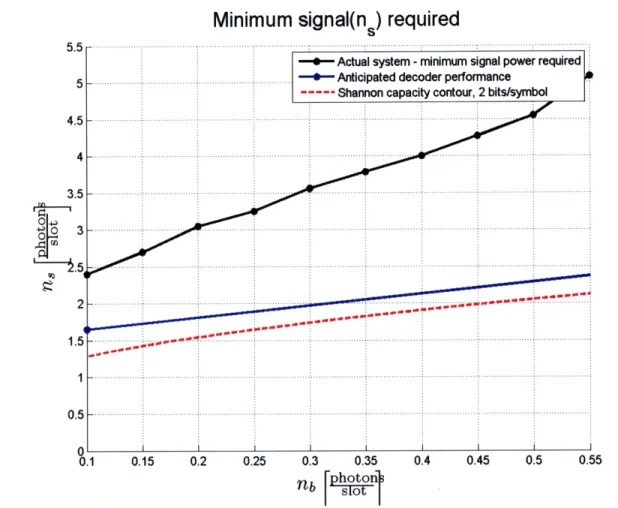
Before a spatial mask can be chosen, the signal and background levels at which the system will not achieve reliable communication must be determined. This problem was approached empirically from the perspective that, given a background level nb, the system needs a minimum amount of signal nsmin in order to successfully decode the received signal. That minimum signal was measured by reducing the signal power at the receiver end of the testbench for a given background power until the SCCC decoder operated at 8 iterations. The results can be found in Table 3.2.

Figure 3-1 plots the data points in Table 3.2, as well as the expected minimum signal required to achieve Shannon capacity. The gap between the two curves can be attributed to nonidealities in the SCCC turbodecoder and timing jitter between the transmitter and receiver, which could cause signal and background photons to be binned incorrectly. However, we note that there is still a large gap between the actual minimum signal required and the signal required by a system with a lossy decoder. Previous implementations of the LLFSO did approach and actually fit the decoder-limited receiver loss. This particular iteration of the testbench system, on which the data n,,smin(nb) was taken, is lossier than an ideal link and a link affected only by decoder loss. However, characterization work has not been performed yet to determine the cause of the increase in nsmin gap between current and previous

LLFSO implementations. However, this pessimistically high estimate for ,,min can still be used in the DPS algorithm as a point mapping to a threshold margin without

affecting its general function.

Minimum signal(ns )

required

5 .5

...

-- Actual system - minimum signal power required

5 -..-. Anticipated decoder performance

--- Shannon capacity contour, 2 bits/symbol 4.5 4-3.5

Figure 3-1: Minimum signal power required to successfully decode at a given back-ground power for the implemented system, for a system with losses due to the SCCC turbodecoder alone, and for the ideal system capable of achieving Shannon capacity.

In terms of n, and nb we can define the link's signal margin at a given spatial

mask to be

.MAsig - - nsmin(nb) (3.7)

= Q sitsiot - nsmin(Q 1 Pbislot) (3.8)

mask mask

(3.9)

Simple and appealing though it may be, it is not clear that Msig is a suitable metric for 46

selecting the data rate and improving decoder performance. By definition, Mi > 0

provides a criterion by which all possible Q factors can be tested to find the maximum

data rate at which the link will have enough signal to achieve decoder convergence. However, the evaluation of the excess signal margin on the link does not correspond to the amount of excess data rate the link has available. In addition, the link data-rate margin is also a more appropriate measure of the decoder performance.

The SCCC turbodecoder implemented in the testbench setup is a max-log-MAP

iterative turbodecoder [21]. Log-likelihood ratios for the raw data in an arriving

symbol are constructed using the derived Poisson channel parameters for the signal and background photons. Then, the decoder evolves a symbol solution by repeatedly passing the log-likelihood ratios through concatenated Soft-Input Soft-Output (SISO) decoders until the decoder as a whole converges to a clear solution [3]. Under these operating parameters, the decoder used in the testbench setup has achieved data rates within 1 dB of the Shannon capacity [13].

In the case of the testbench system's max-log-MAP iterative turbodecoder, the decoder is allowed a maximum of 50 iterations before it must output a decision. The higher the number of iterations the decoder takes to come to a decision, the more stressed it is and the greater the likelihood of an incorrect decoding decision. Given this performance of the decoder as well as the statement that turbocodes belong to the class of codes whose error rates decrease exponentially at data rates less than capacity [5], the number of iterations of the decoder can both be tied to the margin between the channel capacity of the existing link and the data rate at which the system is actually operating.

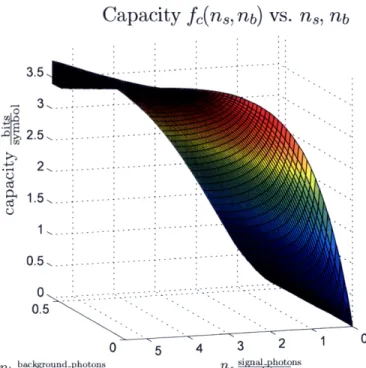
In other words, an appropriate metric can be constructed from the Shannon

chan-nel capacity of the system, written as a function C(ns, nb) of the signal and

back-ground photon numbers, according to

Mcap - C(n, nb) - C(n,,min (nb), nb) (3.10)

while C(ns, nb) will be referred to as the working capacity of the link.

3.4

Review of channel capacity

W X" y"

estimte

messw m of message

Figure 3-2: General block diagram of a communication system. Modified from Ele-ments of Information Theory by Cover and Thomas.

Figure 3-2 shows a block diagram of a communication system in which a set of messages, W, that are mapped into n-bit signals X", are transmitted over a channel which outputs Y'. The behavior of the channel is characterized by a conditional probability distribution p(YIX) when the channel has no memory. The decoder processes the corrupted signal Y" to produce an estimate of the input message, W.

The channel capacity, C, is then the maximum mutual information, I(X, Y), of the channel over all choices of a prior distribution for X, as shown in (3.11) and (3.12).

C = max I(X, Y) (3.11)

p(X)

I(X, Y)= p(X, Y)log( p(X, Y) (3.12)

Xn ,yn

Shannon's Noisy Channel Coding Theorem provides an operational definition of ca-pacity [20]. It states that given a channel caca-pacity of C and a data rate R, there is guaranteed to exist an encoding scheme such that received codewords can be decoded with an arbitrarily small probability of error provided that R < C. The converse to this theorem also states that for R > C it is impossible to transmit data reliably through this channel.

The FSO channel with atmospheric turbulence is time-varying with memory on the order of 1-, where fG is the Greenwood frequency. However, the one second interleaving time employed in the LLFSO system can handle atmospheric fades that range up to approximately 0.5 seconds [13]. The overall channel, therefore, is rendered