HAL Id: hal-00503226
https://hal.archives-ouvertes.fr/hal-00503226
Submitted on 24 Dec 2015
HAL is a multi-disciplinary open access
archive for the deposit and dissemination of
sci-entific research documents, whether they are
pub-lished or not. The documents may come from
teaching and research institutions in France or
abroad, or from public or private research centers.
L’archive ouverte pluridisciplinaire HAL, est
destinée au dépôt et à la diffusion de documents
scientifiques de niveau recherche, publiés ou non,
émanant des établissements d’enseignement et de
recherche français ou étrangers, des laboratoires
publics ou privés.
and temperature
N. P. Gillett, H. Akiyoshi, Slimane Bekki, P. Braesicke, V. Eyring, R. Garcia,
A. Yu. Karpechko, C. A. Mclinden, Olaf Morgenstern, D. A. Plummer, et al.
To cite this version:
N. P. Gillett, H. Akiyoshi, Slimane Bekki, P. Braesicke, V. Eyring, et al.. Attribution of observed
changes in stratospheric ozone and temperature. Atmospheric Chemistry and Physics, European
Geosciences Union, 2011, 11 (2), pp.599-609. �10.5194/acp-11-599-2011�. �hal-00503226�
www.atmos-chem-phys.net/11/599/2011/ doi:10.5194/acp-11-599-2011
© Author(s) 2011. CC Attribution 3.0 License.
Chemistry
and Physics
Attribution of observed changes in stratospheric ozone and
temperature
N. P. Gillett1, H. Akiyoshi2, S. Bekki3, P. Braesicke4, V. Eyring5, R. Garcia6, A. Yu. Karpechko7, C. A. McLinden8,
O. Morgenstern4,9, D. A. Plummer1, J. A. Pyle4, E. Rozanov10,11, J. Scinocca1, and K. Shibata12
1Canadian Centre for Climate Modelling and Analysis, Environment Canada, Victoria, BC, Canada 2National Institute for Environmental Studies, Tsukuba, Japan
3Service d’A´eronomie, Institut Pierre-Simone Laplace, Paris, France
4University of Cambridge, Department of Chemistry, Cambridge/National Centre for Atmospheric Science, UK 5Deutsches Zentrum f¨ur Luft- und Raumfahrt, Institut f¨ur Physik der Atmosph¨are, Oberpfaffenhofen, Germany 6National Center for Atmospheric Research, Boulder, CO, USA
7Finnish Meteorological Institute, Helsinki, Finland 8Environment Canada, Toronto, Canada
9National Institute of Water and Atmospheric Research, Lauder, New Zealand
10Physikalisch-Meteorologisches Observatorium Davos/World Radiation Center, Davos, Switzerland 11Institute for Atmospheric and Climate Science, ETH, Zurich, Switzerland
12Meteorological Research Institute, Tsukuba, Japan
Received: 12 May 2010 – Published in Atmos. Chem. Phys. Discuss.: 16 July 2010 Revised: 3 November 2010 – Accepted: 1 January 2011 – Published: 20 January 2011
Abstract. Three recently-completed sets of simulations of
multiple chemistry-climate models with greenhouse gases only, with all anthropogenic forcings, and with anthro-pogenic and natural forcings, allow the causes of observed stratospheric changes to be quantitatively assessed using de-tection and attribution techniques. The total column ozone response to halogenated ozone depleting substances and to natural forcings is detectable in observations, but the to-tal column ozone response to greenhouse gas changes is not separately detectable. In the middle and upper strato-sphere, simulated and observed SBUV/SAGE ozone changes are broadly consistent, and separate anthropogenic and nat-ural responses are detectable in observations. The influence of ozone depleting substances and natural forcings can also be detected separately in observed lower stratospheric tem-perature, and the magnitudes of the simulated and observed responses to these forcings and to greenhouse gas changes are found to be consistent. In the mid and upper stratosphere the simulated natural and combined anthropogenic responses are detectable and consistent with observations, but the influ-ences of greenhouse gases and ozone-depleting substances could not be separately detected in our analysis.
Correspondence to: N. P. Gillett
1 Introduction
As concentrations of anthropogenic halogenated Ozone De-pleting Substances (ODSs) peak in the stratosphere and begin to fall, greenhouse gas (GHG) increases are expected to be-come an increasingly important driver of future stratospheric ozone trends (e.g. WMO, 2007), hence the evolution of ozone as ODSs decrease is not expected to be a simple rever-sal of historical trends (e.g. Jonsson et al., 2009; Waugh et al., 2009). The projections of future ozone evolution contained in the recent WMO Ozone Assessment (WMO, 2011) rely heavily on three-dimensional chemistry-climate models, and on the realism of their simulated ozone response to green-house changes. However, while historical trends in total column ozone simulated in response to combined ODS and greenhouse gas forcings have been shown to be reasonably consistent with observations, (Chapter 3 of SPARC CCMVal, 2010; Karpechko et al., 2010), the simulated stratospheric temperature and ozone response to greenhouse gases in these models has not previously been directly tested against obser-vations. ODSs have been the dominant driver of past strato-spheric ozone changes, and ozone changes have been the dominant driver of lower stratospheric temperature changes (WMO, 1999; Shine et al., 2003; Santer et al., 2003; Cordero and Forster, 2006; Ramaswamy et al., 2006). Until recently, few chemistry-climate simulations of the response to green-house gas changes alone had been performed.
Waugh et al. (2009) examine the influence of greenhouse gas changes on total column ozone in a transient chemistry-climate simulation. They find that the rise in greenhouse gases leads to column ozone decreases in the tropics, in-creases in the northern midlatitudes and little change in the Southern Hemisphere, with ODSs the dominant influence over the historical period, which is our focus here. The largest greenhouse gas contributions to ozone mixing ratio change are in the tropical lower stratosphere, where green-house gas increases drive decreases in ozone mixing ratio, due to a strengthening Brewer-Dobson circulation, and in the tropical upper stratosphere, where rising greenhouse gas concentrations increase ozone mixing ratio by a cooling-induced reduction in gas phase depletion, consistent with earlier CCM simulations of the equilibrium response to dou-bled CO2(e.g. Jonsson et al., 2004; Fomichev et al., 2007),
and two dimensional model results (e.g. Haigh and Pyle, 1982). Plummer et al. (2010) show similar effects of house gases on ozone in simulations of CMAM with green-house gas changes only. Jonsson et al. (2009) also reach similar conclusions by using a regression model to sepa-rate the ozone response to ODSs and greenhouse gases in a chemistry-climate simulation in which changes in both were included. However, none of these studies make quantitative comparisons of the simulated ozone changes in response to each forcing and the actual changes observed, in order to test whether there is evidence of an ozone response to greenhouse gases in the real world, and indeed whether the simulated ozone changes are consistent with the observations.
Stratospheric temperature is an important driver of strato-spheric ozone change, and a variable of interest in its own right. Several studies have examined the causes of strato-spheric temperature change in chemistry-climate models (Jonsson et al., 2009; Plummer et al., 2010; Stolarski et al., 2010), and others have compared trends in GCMs with lim-ited stratospheric resolution and prescribed ozone changes with observations (Santer et al., 2003; Cordero and Forster, 2006; Ramaswamy et al., 2006). These studies have gener-ally concluded that ozone or ODSs have been the dominant driver of observed lower stratospheric cooling. Higher in the stratosphere, greenhouse gases have played a more im-portant role (e.g. Shine et al., 2003; Jonsson et al., 2009; Stolarski et al., 2010). There is a difference between parti-tioning the temperature trend into ozone-induced and GHG-induced changes, and partitioning it into ODS-GHG-induced and GHG-induced changes (Shepherd and Jonsson, 2008; Jon-sson et al., 2009). The latter approach, which we follow here, leads to a smaller temperature change being attributed to greenhouse gases, because the GHG-cooling-induced in-crease in ozone concentration cancels out part of the cool-ing due the GHGs themselves (Shepherd and Jonsson, 2008). Here we make use of newly-completed Chemistry-Climate Model Validation (CCMVal) activity simulations with green-house gas changes only (Eyring et al., 2010), as well as ear-lier sets of simulations with anthropogenic and combined
anthropogenic and natural forcings (Chapter 2 of SPARC CCMVal, 2010), to examine the causes of observed changes in stratospheric ozone and temperature, and to test for con-sistency between models and observations.
2 Data and models
We mainly use output from three sets of CCMVal simula-tions (Chapter 2 of SPARC CCMVal, 2010): one includ-ing anthropogenic (ODSs and GHGs, but not tropospheric aerosols) and natural forcings (solar cycle, volcanic aerosols and QBO in most models) (REF-B1), one including anthro-pogenic forcings only (REF-B2), and one including green-house gas changes only (SCN-B2b) (Table 1). Output was taken from seven CCMVal models which had output from all three simulations over the period 1979–2005. Output from the ULAQ model was not used due to apparently unrealis-tic ozone changes in its SCN-B2b simulation (Eyring et al., 2010). The ensemble size for each model was chosen such that an equal number of simulations from each model was used with each set of forcings: this resulted in a single en-semble member for all models except for CMAM, which had an ensemble size of three, giving a total of nine simulations for each set of forcings.
The response to the well-mixed greenhouse gases car-bon dioxide, methane and nitrous oxide (GHG) was evalu-ated directly from the SCN-B2b simulations, the ODS re-sponse was evaluated by subtracting the SCN-B2b simula-tions from the REF-B2 simulation, and the natural forcing response (NAT) was evaluated by subtracting the REF-B2 simulation from the REF-B1 simulation. As well as the ef-fect of changes in well-mixed greenhouse gases in the atmo-sphere, the calculated GHG response also includes the effect of specified SST changes from separate coupled atmosphere-ocean GCMs with prescribed anthropogenic forcing, or in the case of CMAM, coupled SST changes. The three CMAM simulations and the UMUKCA-UCAM simulation included the radiative effects of changes in ODSs in the SCN-B2b simulations, while the other models excluded them. Thus in the SCN-B2b simulations, these two models used differ-ent ODS forcings in the radiation and chemistry schemes. A comparison of the lower stratospheric temperature trends in the SCN-B2b simulations with and without the radiative fects of ODSs indicated that simulations including these ef-fects tended to warm more in the lower latitudes compared to those excluding them (Forster and Joshi, 2005), though the differences were not generally statistically significant. The GHG response thus includes roughly half the radiative re-sponse to ODSs, with the other half included with the cal-culated response to ODSs themselves. Changes in certain ozone precursors were also prescribed (Chapter 2 of SPARC CCMVal, 2010; Morgenstern et al., 2010) in all simula-tions, and hence their effects are included with the GHG re-sponse. CCSRNIES, MRI, SOCOL, UMUKCA-UCAM and
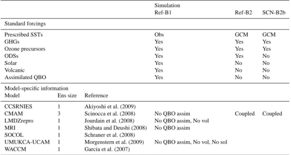
Table 1. CCMVal simulations used. The maximum possible ensemble size “Ens size” was chosen for each model such that the ensemble size
was the same for all three simulations, in order to avoid aliasing model differences into differences between multi-model means of simulations with different forcings. “No QBO assim” indicates that no QBO was assimilated. MRI and UMUKCA-UCAM have an internally generated QBO, and CMAM and LMDZrepro do not simulate the QBO. “No vol” indicates that direct radiative effects of volcanic aerosol were not included, although the chemical effects were included in all models. “No sol” indicates that no solar cycle was specified. “Coupled” indicates that the atmosphere model was coupled to a dynamical ocean model.“GHGs” refers to to the greenhouse gases carbon dioxide, methane and nitrous oxide.
Simulation
Ref-B1 Ref-B2 SCN-B2b Standard forcings
Prescribed SSTs Obs GCM GCM
GHGs Yes Yes Yes
Ozone precursors Yes Yes Yes
ODSs Yes Yes No
Solar Yes No No
Volcanic Yes No No
Assimilated QBO Yes No No
Model-specific information
Model Ens size Reference
CCSRNIES 1 Akiyoshi et al. (2009)
CMAM 3 Scinocca et al. (2008) No QBO assim Coupled Coupled LMDZrepro 1 Jourdain et al. (2008) No QBO assim, No vol
MRI 1 Shibata and Deushi (2008) No QBO assim SOCOL 1 Schraner et al. (2008)
UMUKCA-UCAM 1 Morgenstern et al. (2009) No QBO assim, No vol, No sol WACCM 1 Garcia et al. (2007)
WACCM have simplified background tropospheric chem-istry schemes, and in these models tropospheric ozone likely increases somewhat in response to these emissions. Fol-lowing Waugh et al. (2009) and Plummer et al. (2010), the ODS response was evaluated by differencing the REF-B2 and SCN-B2b simulations. As well as the chemical effects of ODSs this difference also includes the radiative effects of the ODSs in four of the nine simulations (the radiative effects of ODSs are not included in any of the MRI simulations).
Lastly the natural forcing (NAT) response was evaluated by differencing the REF-B1 and REF-B2 sets of simulations: the NAT response thus includes the simulated response to so-lar and volcanic forcing in most models (Table 1), and the ef-fects of an assimilated QBO in three of the nine simulations. It also includes the additional effects of prescribing observed SSTs (in the REF-B1 simulations), rather than SSTs simu-lated in response to anthropogenic forcings with a separate coupled atmosphere-ocean GCM or predicted with the cou-pled model in the case of CMAM (in the REF-B2 simula-tions). A comparison of the warming at 400 hPa (the lowest level on which data were available from all models) indicates that the REF-B2 simulations warmed by about 0.2 K more than the REF-B1 simulations over the 1979–2005 period at this level after masking out post-volcano years – this indi-cates that the SSTs in the REF-B2 simulations likely warm somewhat more than the observed SSTs used in the REF-B1 simulations in these models. Any stratospheric response to the weaker tropospheric warming in the REF-B1
simula-tions would thus be captured in the NAT signal, as would any stratospheric response to ENSO.
This analysis assumes that the stratospheric temperature and ozone response to individual forcings add linearly: McLandress et al. (2010) demonstrate that this is a valid as-sumption for stratospheric temperature. Eyring et al. (2010) find this assumption to hold for ozone in most regions, but with some departures from linearity in tropical column ozone. In our approach any nonlinearity arising from the combined effects of ODSs and GHGs would be included with the ODS response. To check the linearity assumption, we also repeated our attribution analysis for lower stratospheric temperature and total column ozone using the fixed green-house gas SCN-B2c simulations (Eyring et al., 2010), avail-able for all models but UMUKCA-UCAM, to derive the ODS response directly. These simulations generally have fixed carbon dioxide, methane and nitrous oxide in the chemistry and radiation schemes, with the exception of CMAM which allows these gases to vary in the chemistry scheme (Plummer et al., 2010). ODSs are time-varying in the chemistry scheme in all cases, and in the radiation scheme in all models except CMAM. These differences in the treatment of the gases in CMAM are the main reason that we focus our analysis on the SCN-B2b simulations, but nonetheless these simulations represent a useful check on our results. When using these simulations, we evaluate the NAT response by subtracting the SCN-B2b and SCN-B2c simulations from the REF-B1 simulations.
In the absence of sufficiently long unforced control simu-lations, internal variability was estimated by taking the full length of each ensemble (1960–2005 in the case of the REF-B1 simulations, and 1960 until the mid to late 21st century in the case of the REF-B2 and SCN-B2b simulations), subtract-ing the multi-model ensemble mean, multiplysubtract-ing by √9/8 to inflate the variance to account for this subtraction of the multi-model ensemble mean (Stone et al., 2007), and then sampling 27-year segments (corresponding to the length of our analysis period) of the resulting anomalies starting at 5-year intervals. The variance-inflation step is necessary be-cause subtracting an ensemble mean removes some of the in-ternal variability as well as the forced response. Means were then subtracted from each 27-year segment. This method almost certainly results in higher estimated variability than using a control simulation, since inter-model differences in forced response will be aliased into the variability. This makes the approach conservative for detection, since indi-vidual forced responses are less likely to be detected than with a standard attribution analysis using a control simula-tion. However, this also has the effect of making the test for consistency between observations and models more permis-sive, since some component of model uncertainty is added to the variability estimate.
Simulated stratospheric ozone changes were compared with two observational data sets: a dataset of monthly mean column ozone from merged Total Ozone Mapping Spectrom-eter (TOMS) and Solar Backscatter Ultraviolet (SBUV) mea-surements (available at http://acdb-ext.gsfc.nasa.gov/Data services/merged/), and a SAGE-corrected SBUV dataset of monthly mean zonal mean ozone anomalies on 11 pressure levels from ∼50 hPa to ∼0.5 hPa (McLinden et al., 2009). Two satellite-derived stratospheric temperature datasets were used: a record of monthly mean lower stratospheric temper-atures derived from Microwave Sounding Unit (MSU) and Advanced Microwave Sounding Unit (AMSU) observations (Mears and Wentz, 2009), and a dataset of zonal mean tem-peratures from the Stratospheric Sounding Unit (SSU) (Ran-del et al., 2009). Only the directly-observed channels 25, 26 and 27 were used in this analysis, and not the X-channels, which are subject to larger uncertainties (Randel et al., 2009). All model output was averaged on the observational grid, and then masked with observational data coverage before means were calculated. The original SAGE-corrected SBUV timeseries were converted from ozone partial column to vol-ume mixing ratio by calculating the partial column of air in SBUV layers using the same atmospheres (and hence the same temperature trends) that were used in deriving the origi-nal dataset. Volume mixing ratio was then calculated by tak-ing the ratio of ozone partial column to air partial column, and was interpolated onto CCMVal output pressure levels. Model zonal mean temperatures were weighted with MSU and SSU weighting functions to generate synthetic layer tem-peratures for comparison with observations. Lower strato-spheric temperature trends evaluated from the models were
found to be sensitive to the details of the weighting function used: we used the high-resolution weighting function pro-vided by Remote Sensing Systems (Mears and Wentz, 2009). All analysis was carried out over the 27-year period from 1979 to 2005, since most of the observations start in 1979, and the REF-B1 simulations finish in 2005.
3 Results
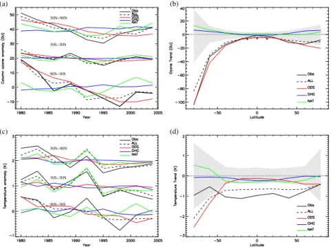
Figure 1a compares the evolution of 3-yr mean anomalies of total column ozone over the tropics, NH extratropics and SH extratropics, and Fig. 1b compares zonal mean trends in column ozone, calculated from the 3-yr means. Overall the agreement appears good between the observations and the total ozone anomalies simulated in response to combined an-thropogenic and natural forcings (ALL, corresponding to the REF-B1 simulations) (Chapter 3 of SPARC CCMVal, 2010). ODSs clearly exert the dominant influence on ozone in the extratopics in the model, with the largest decreases at high latitudes, particularly in the SH, and this pattern is also ap-parent in the observations. GHGs exert a relatively weak in-fluence over this period in the model, with decreases in the tropics and increases at high latitudes, likely related to an acceleration of the Brewer-Dobson circulation (Chapter 4 of SPARC CCMVal, 2010). Natural forcings exert little influ-ence on the trends, but their influinflu-ence in the models is appar-ent in the anomalies.
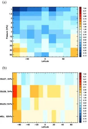
In order to objectively test the consistency of the simulated and observed evolution of column ozone, and in order to test for the presence of a response to ODSs, GHGs and natural forcings in the observations, we applied a detection and attri-bution analysis. Before applying a formal attriattri-bution analysis to the observed trends, it is necessary to check whether the simulated variability is realistic. Figure 2a shows the ratio of simulated to observed variances in monthly and annual total column ozone anomalies at each latitude. Simulated variabil-ity tends to be larger than observed at high latitudes (some individual models have high-biased variance, and some have low-biased variance, but on average the variance is higher than observed), making detection results conservative.
In order to carry out a detection and attribution analysis, we assume that the total column ozone observations, y (an 81-element vector containing nine 3-yr mean anomalies over nine 20◦ zonal bands), may be written as a linear sum of the simulated responses to individual forcings (xODS, xGHG,
xNAT), each scaled by a regression coefficient (βODS, βGHG,
βNAT), plus residual variability, u:
y = βODSxODS+βGHGxGHG+βNATxNAT+u (1)
After projecting onto the 40 leading EOFs of internal vari-ability, regression coefficients were evaluated using a to-tal least squares optimal regression to account for inter-nal variability in the observations and in the simulated re-sponses (Allen and Stott, 2003; Hegerl et al., 2007), and
30N!90N (a) (b) (c) (d) 30N!90N 90S!30S 30S!30N 90S!30S 30S!30N
Fig. 1. Comparison of simulated and observed changes in total column ozone (a and b) and lower stratospheric temperature (c and d).
Panel (a) shows 3-yr mean total column ozone anomalies from a merged TOMS/SBUV dataset and simulated in response to ODS, GHG,
NAT and all forcings combined over three zonal bands in DU. Anomalies for 30◦S–30◦N and 30◦N–90◦N are offset by 20 DU and 40 DU
respectively. Zonal mean least-squares linear trends in total column ozone in observations and simulated in response to each forcing are shown in (b) in DU over the 27-period 1979–2005. Grey bands show the estimated 5th–95th percentile ranges of internal variability. Black crosses in (b) show stratospheric column ozone trends estimated from TOMS data using the convective cloud differential method (Ziemke et al., 1998). (c) and (d) are equivalent plots for MSU lower stratospheric temperature, in K over the 27-yr period 1979–2005. Anomalies for 30◦S–30◦N and 30◦N–90◦N are offset by 1 K and 2 K respectively in (c).
area-weighting was used. EOFs were evaluated from half of the intra-ensemble anomaly segments described previously, based on the same diagnostic of nine 3-yr mean anomalies over nine 20◦zonal bands. The choice of EOF truncation is somewhat arbitrary: The number of EOFs needs to be high enough to represent the main features of the simulated re-sponse patterns, but not too high since simulated variability in the highest order EOFs is often underestimated (Allen and Tett, 1999). The results presented here were not sensitive to moderate variations in the EOF truncation, except where noted in the text.
The remaining intra-ensemble anomaly segments were used to assess the uncertainty in the regression coefficients. A regression coefficient which is significantly greater than zero indicates a detectable response to the forcing concerned: The projection of the observations onto the simulated re-sponse to this forcing is inconsistent with simulated internal variability. A regression coefficient consistent with one in-dicates simulated and observed responses to the forcing con-cerned of a consistent magnitude. The attribution of an ob-served change to a given combination of forcings requires a demonstration both that the observed change is inconsistent with internal variability, and that it is consistent with the sim-ulated response to the given set of forcings, where all
plau-sible alternative explanations for the change have been ruled out (Mitchell et al., 2001).
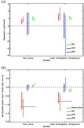
Figure 3a shows the regression coefficients for total col-umn ozone on the left. The residual observed variability, u, was found to be consistent with simulated internal variabil-ity (Allen and Tett, 1999), and similar results were obtained for EOF truncations in the range 20–45. Regression coeffi-cients for ODS and NAT are inconsistent with zero (5–95% error bars do not cross the zero line), indicating that the ob-served response is inconsistent with internal variability, and a response to ODS and NAT is detectable in the column ozone observations. While the NAT regression coefficient is consis-tent with one, indicating a simulated and observed response of consistent magnitude, the ODS regression coefficient ap-pears to be less than one, suggesting that the ODS response is overestimated by the models. This inconsistency was not, however, apparent when the ODS response was evaluated di-rectly from simulations with fixed greenhouse gas concen-trations (SCN-B2c, Eyring et al., 2010), as shown by the light shaded bars in Fig. 3a, or for EOF truncations below 35, suggesting that this is not a robust difference between simulations and observations. As expected, ODSs are the main driver of the observed decrease in total column ozone (Fig. 3b). The GHG response is not detected (its regression
(b) (a)
Fig. 2. Ratios of simulated to observed variances in (a) total
col-umn ozone and (b) MSU lower stratospheric temperature, as a func-tion of latitude. Solid lines show the ratio of variances of monthly means, and dashed lines show the ratio of variances of annual means. Variances are calculated over the 1979–2005 period without detrending, and simulated variances are taken from the unfiltered ALL (REF-B1) simulations.
coefficient is not inconsistent with zero), but the simulated and observed GHG responses are not inconsistent in magni-tude. At some truncations above 45, or if the UMUKCA-UCAM model is excluded from the analysis, there is evi-dence of an apparent inconsistency in the simulated and ob-served GHG response, but this difference appears not to be robust.
Closer examination of Fig. 1b indicates that the model re-sponse to the combined forcings overestimates the decrease in ozone in the tropics, as was also found in CMAM (Plum-mer et al., 2010). One possible reason for this apparent difference between observations and the simulations is that the CCMVal simulations used here either have simplified background tropospheric chemistry (CCSRNIES, MRI, SO-COL, UMUKCA-UCAM and WACCM) or no tropospheric chemistry at all (CMAM and LMDZrepro), and therefore the ensemble is not expected to realistically simulate changes in tropospheric ozone due to increases in the emissions of ozone precursors (Forster et al., 2007; Staehelin and Schnadt Poberaj, 2008). While extratropical tropospheric column ozone trends are uncertain, and only measured in a few
loca-(b) (a)
Fig. 3. (a) Regression coefficients of observed changes in
to-tal column ozone (left) and lower stratospheric temperature (right) onto the simulated responses to ozone depleting substances (ODS), greenhouse gases (GHG) and natural forcings (NAT). Dark bars show results derived using the REF-B1, REF-B2 and SCN-B2b simulations, and light bars show results derived using the REF-B1, SCN-B2b and SCN-B2c simulations. Bars represent 5–95% uncer-tainty ranges. In both cases results are based on nine 3-yr means
over nine 20◦zonal bands, and use a representative EOF truncation
of 40. Similar results were obtained using 2-yr means. (b) Trends in global mean total ozone (dDU/27 yr) and lower stratospheric temperature (K/27 yr) over the period 1979–2005 attributable to each forcing, derived from the attribution analysis (Allen and Stott, 2003). Horizontal black lines show the observed trends.
tions, separate estimates of the tropospheric and stratospheric contributions to column ozone trends have been made for 15◦S–15◦N using TOMS data (Ziemke et al., 1998), and the stratospheric components of the trends are shown in Fig. 1b (black crosses). These clearly show larger decreasing trends over the period considered compared to the total column, pre-sumably due to tropospheric ozone increases, perhaps due to enhanced biomass burning (Staehelin and Schnadt Poberaj, 2008). These are in closer agreement with the ALL simula-tions.
Figure 1c and d show changes in MSU lower strato-spheric temperature, a layer whose weighting function peaks at 83 hPa. Agreement between the ALL simulations and observations is generally good, although the observations show a relatively uniform cooling trend across latitude bands
(d) GHG
(a) OBS (b) ALL
(c) ODS
Fig. 4. Zonal mean linear least-squares trends in ozone (change over the period 1979–2005 expressed as a percentage of the observed 1979–
2005 climatology) in SAGE-corrected SBUV observations (McLinden et al., 2009) (a), and simulated in response to combined anthropogenic and natural forcings (b), ODS changes (c), and GHG changes (d).
(Randel et al., 2009), while the ALL response shows en-hanced cooling over the Antarctic. This lack of Antarctic cooling in the observations is only partially explained by the inclusion of data from 2002, a year with the only known occurrence of an Antarctic sudden stratospheric warming (Varotsos, 2002; Allen et al., 2003). Randel et al. (2009) show that zonal mean MSU lower stratospheric temperature over the Antarctic has cooled in November and December, but has warmed in the winter and early spring, leading to only a small cooling in the annual mean. Lin et al. (2009) demonstrate that an ozone-induced radiative cooling dur-ing the sprdur-ing at around 45◦W at high southern latitudes is largely balanced by a dynamical warming at around 135◦E in the observations. Lin et al. (2009) also show that the CMIP3 models, by contrast, show a zonally uniform enhanced high latitude cooling in simulations including stratospheric ozone changes. Our results suggest that the CCMVal models re-spond similarly. The stratospheric warming following the eruptions of El Chich´on (1982) and Pinatubo (1991) is ap-parent in the observations and the ALL and NAT responses, and solar variations likely also contribute to lower strato-spheric temperature variability (Randel et al., 2009). Vari-ability in simulated lower stratospheric temperature is some-what overestimated compared to observations, particularly at high southern latitudes (Fig. 2b), which is consistent with a high bias in simulated variability in stratospheric zonal mean wind in the CCMVal-2 simulations in Antarctic
sum-mer (Chapter 10 of SPARC CCMVal, 2010): this will tend to make detection results conservative.
An optimal regression applied to lower stratospheric tem-perature, using the same method as for total column ozone, yielded clearly detectable ODS and NAT signals, and a GHG signal which was not detectable (Fig. 3a). However, there is no evidence of inconsistency in the magnitude of the simu-lated and observed GHG response, since its regression co-efficient is consistent with one. A residual test was passed, indicating consistency between simulated and observed vari-ability (Allen and Tett, 1999). Thus ODS and NAT influ-ences are clearly identifiable in observed lower stratospheric temperatures, and simulated and observed responses are con-sistent in amplitude. ODSs are the dominant contributor to the long term cooling trend (Fig. 3b), with NAT contribut-ing a small but significant coolcontribut-ing trend. The small NAT cooling is likely due to the fact that El Chich´on warmed the stratosphere in the first half of the record, while there were no volcanic eruptions in the second half of the record, result-ing in a coolresult-ing trend due to natural forcresult-ing (Fig. 1c). The warming due to Pinatubo occurred close to the centre of the record, therefore it had little effect on the 1979-2005 trend (Fig. 1c). These results are consistent with previous results based on tropospheric GCMs (Santer et al., 2003; Cordero and Forster, 2006; Ramaswamy et al., 2006).
Our analysis up to this point has focused on lower stratospheric variations in ozone and temperature: next we
(b) (a)
Fig. 5. Ratios of simulated to observed variances in (a) ozone
mix-ing ratio and (b) MSU and SSU layer temperatures, as a function of latitude and pressure. Variances were calculated from monthly anomalies over the 1979–2005 period, and simulated variances were taken from the ALL simulations.
consider vertically-resolved ozone and temperature varia-tions extending into the upper stratosphere. Figure 4 com-pares observed ozone trends from an SBUV dataset (McLin-den et al., 2009) with the simulated response to ODS, GHG and ALL. In the models the ozone trends are clearly driven primarily by ODSs, with GHGs contributing a small decrease in the tropical lower stratosphere, and a small increase else-where. The ALL response and the observations exhibit rel-atively good agreement, although the models somewhat un-derestimate the trends in the upper stratosphere. Steinbrecht et al. (2009) compare CCMVal-1 REF-B1 simulated ozone with observations at selected midlatitude and tropical lo-cations at 35–45 km altitude, and report broad consistency. Simulated monthly variability in these ozone mixing ratios was generally somewhat smaller than that found in the SBUV dataset (Fig. 5a), though the models showed larger variabil-ity than observed over the poles in the lower stratosphere, consistent with results for total ozone (Fig. 2a). Part of the discrepancy in the tropics is associated with the QBO: mod-els including an assimilated QBO show variability broadly consistent with observations below 10 hPa, though they also underestimate variability somewhat above this (not shown).
Fig. 6. Regression coefficients of observed changes in SBUV
strato-spheric ozone mixing ratio (left) and SSU stratostrato-spheric tempera-ture (right) onto the simulated responses to anthropogenic forcings (ANT) and natural forcings (NAT). The ANT response was derived from the REF-B2 output. Results are based exclusively on those models in which a QBO was assimilated (CCSRNIES, SOCOL and WACCM). Bars represent 5–95% uncertainty ranges. SBUV results
are based on nine 3-yr means over nine 20◦zonal bands on eleven
levels, and SSU results are based on nine 3-yr means over fifteen
10◦zonal bands on three levels, and both use a representative EOF
truncation of 40.
In order to apply an attribution analysis to SBUV ozone, we restricted our attention to those models which included an assimilated QBO (CCSRNIES, SOCOL and WACCM): these models exhibit more realistic ozone variability, and de-riving a NAT response from a combination of models with and without a QBO would lead to a too-weak NAT response by construction which would bias regression results. Per-haps due to the limited ensemble size and lack of statis-tical independence between the ODS and GHG responses, it was not possible to robustly separate ODS and GHG re-sponses in SBUV ozone, and similar results were obtained when restricting the analysis to the tropics, NH extratrop-ics or SH extratropextratrop-ics. However a combined anthropogenic (ANT) response and the NAT response were clearly de-tectable (Fig. 6). The ANT response was of a consistent magnitude in simulations and observations, but the NAT re-gression coefficient was significantly greater than one, indi-cating that the NAT response is somewhat too weak in the models. The QBO in these models is assimilated by nudging zonal wind, and even in zonal wind itself the QBO amplitude in these models is too weak (Chapter 4 of SPARC CCMVal, 2010), thus the ozone response to the QBO might also be expected to be underestimated.
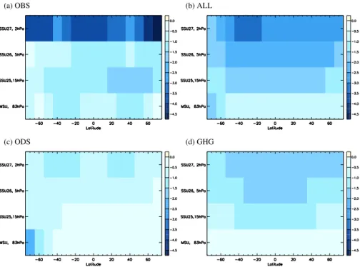
Lastly we compare observed SSU zonal mean tempera-ture trends on three layers in the mid and upper stratosphere (Fig. 7). In the models GHGs cause 55–75% of the global mean cooling on the SSU levels, with ODSs also important, broadly consistent with Shine et al. (2003) who compare observed 1980–2000 trends with the simulated response to prescribed GHG changes and stratospheric ozone changes. However, differences are apparent between the simulated
(d) GHG
(a) OBS (b) ALL
(c) ODS
Fig. 7. Zonal mean linear least-squares trends in stratospheric temperature (K over the period 1979–2005) in SSU and MSU observations
(Randel et al., 2009) (a), and simulated in response to combined anthropogenic and natural forcings (b), ODS changes (c), and GHG changes
(d). The name of each channel and the approximate pressure of the maximum in its weighting function are shown on the y-axis.
ALL and observed trends, with the models apparently over-estimating the SSU 26 trends and underover-estimating the SSU 27 trends. Similar results are seen in the global mean (Chap-ter 3 of SPARC CCMVal, 2010). These apparent discrep-ancies could also arise from errors in the observations. Vari-ability in SSU temperatures is broadly consistent between the models and observations (Fig. 5b), with some overestimation of variability in the models at high southern latitudes. As for SBUV ozone, it was necessary to choose only those mod-els which included an assimilated QBO (CCSRNIES, SO-COL and WACCM) for an attribution analysis of mid- and upper-stratospheric temperature: averaging simulations with and without a simulated QBO would create a weak bias in the NAT response. A detection and attribution analysis applied to SSU 25, 26, and 27 temperatures yielded clearly detectable ANT and NAT responses of a consistent magnitude in obser-vations and simulations (Fig. 6). ODS and GHG responses could not be robustly separated in the regression, possibly due to the small ensemble size.
4 Conclusions
Total column ozone changes simulated in response to com-bined anthropogenic and natural forcings are broadly con-sistent with observations, but while the ODS and natural re-sponses are detectable in the observations, the GHG response is not detectable. In the mid and upper stratosphere, the
simu-lated ozone response to anthropogenic forcings is consistent with observations, though the response to natural forcings appears to be somewhat underestimated. Variability in ozone appears to be somewhat underestimated in the upper strato-sphere in the models.
We find a clearly detectable influence of ODSs and natural forcings on lower stratospheric temperature, with the magni-tudes of the simulated responses to ODSs, GHGs and natural forcings consistent with observations. ODSs explain most of the observed lower stratospheric cooling, with natural forc-ings also contributing to the cooling over the period 1979– 2005. Higher in the stratosphere a natural signal and a com-bined anthropogenic signal in temperature are detectable, but ODS and GHG influences are not separately detectable in the SSU observations. We conclude that while the influences of ODSs and natural forcings are clearly detectable in strato-spheric ozone and temperature observations, the influence of greenhouse gas increases is not yet clearly identifiable. A ro-bust separation of the ODS and GHG responses may require a longer period of observations.
Acknowledgements. We thank S. Solomon for proposing this
analysis and for fruitful discussions. We acknowledge the
Chemistry-Climate Model Validation (CCMVal) Activity for the WCRP’s (World Climate Research Programme’s) SPARC (Stratospheric Processes and their Role in Climate) project for organizing and coordinating the model data analysis activity, and the British Atmospheric Data Centre (BADC) for collecting and archiving the CCMVal model output. The CCSRNIES and MRI
simulations were carried out on the supercomputer at the National Institute for Environmental Studies, Japan. CCSRNIES research was supported by the Global Environmental Research Fund of the Ministry of the Environment of Japan (A-071 and B-093). UMUKCA-UCAM simulations made use of HECToR, the UK’s national highperformance computing service, which is provided by UoE HPCx Ltd. at the University of Edinburgh, Cray Inc. and NAG Ltd., and funded by the Office of Science and Technology
through the EPSRC’s High End Computing Programme. MSU
data were produced by Remote Sensing Systems, sponsored
by the NOAA Climate and Global Change Program. Data are
available at www.remss.com. NPG acknowledges support from the International Detection and Attribution group funded by the US department of Energy’s Office of Science, Office of Biological and Environmental Research and the US National Oceanic and Atmospheric Administration’s Climate Program Office. This work is also partly supported by the NOAA Climate and Global Change Program, NOAA Award No. NA08OAR4310729.
Edited by: T. J. Dunkerton
References
Akiyoshi, H., Zhou, L. B., Yamashita, Y., Sakamoto, K., Yoshiki, M., Nagashima, T., Takahashi, M., Kurokawa, J., Takigawa, M., and Imamura, T.: A CCM simulation of the breakup of the Antarctic polar vortex in the years 1980–2004 under the CCMVal scenarios, J. Geophys. Res., 114, D03103, doi:10.1029/ 2007JD009261, 2009.
Allen, M. R. and Stott, P. A.: Estimating signal amplitudes in opti-mal fingerprinting, Part I: Theory, Clim. Dynam., 21, 477–491, 2003.
Allen, M. R. and Tett, S. F. B.: Checking for model consistency in optimal fingerprinting, Clim. Dynam., 15, 419–434, 1999. Allen, D. R., Bevilacqua, R. M., Nedoluha, G. E., Randall, C. E.,
and Manney, G. L.: Unusual stratospheric transport and mixing during the 2002 Antarctic winter, Geophys. Res. Lett., 30, 1599, doi:10.1029/2003GL017117, 2003.
Cordero, E. C. and Forster, P. M. de F.: Stratospheric variability and trends in models used for the IPCC AR4, Atmos. Chem. Phys., 6, 5369–5380, doi:10.5194/acp-6-5369-2006, 2006.
Eyring, V., Cionni, I., Bodeker, G. E., Charlton-Perez, A. J., Kinni-son, D. E., Scinocca, J. F., Waugh, D. W., Akiyoshi, H., Bekki, S., Chipperfield, M. P., Dameris, M., Dhomse, S., Frith, S. M., Garny, H., Gettelman, A., Kubin, A., Langematz, U., Mancini, E., Marchand, M., Nakamura, T., Oman, L. D., Pawson, S., Pitari, G., Plummer, D. A., Rozanov, E., Shepherd, T. G., Shi-bata, K., Tian, W., Braesicke, P., Hardiman, S. C., Lamarque, J. F., Morgenstern, O., Pyle, J. A., Smale, D., and Yamashita, Y.: Multi-model assessment of stratospheric ozone return dates and ozone recovery in CCMVal-2 models, Atmos. Chem. Phys., 10, 9451–9472, doi:10.5194/acp-10-9451-2010, 2010.
Fomichev, V. I., Jonsson, A. I., de Grandpr´e, J., Beagley, S. R., McLandress, C., Semeniuk, K., and Shepherd, T. G.: Response
of the middle atmosphere to CO2 doubling: Results from the
Canadian Middle Atmosphere Model, J. Climate, 20, 1121– 1144, 2007.
Forster, P. M. de F. and Joshi, M.: The role of halocarbons in the cli-mate change of the troposphere and stratosphere, Clim. Change,
71, 249–266, 2005.
Forster, P., Ramaswamy, V., Artaxo, P., Bernsten, T., Betts, R., Fa-hey, D. W., Haywood, J., Lean, J., Lowe, D. C., Myhre, G., Nganga, J., Prinn, R., Raga, G., Schulz, M., and Van Dorland, R.: Changes in atmospheric constituents and in radiative forcing, in: Climate change 2007: The physical science basis, edited by: Solomon, S., Qin, D., Manning, M., Chen, Z., Marquis, M., Av-eryt, K. B., Tignor, M., and Miller, H. L., chap. 2, Cambridge Univ. Press, 129–234, 2007.
Garcia, R. R., Marsh, D. R., Kinnison, D. E., Boville, B. A., and Sassi, F.: Simulation of secular trends in the middle at-mosphere, 1950–2003, J. Geophys. Res., 112, D09301, doi: 10.1029/2006JD007485, 2007.
Haigh, J. D. and Pyle, J. A.: Ozone perturbation experiments in a two-dimensional circulation model, Q. J. Roy. Meteorol. Soc., 108, 551–574, 1982.
Hegerl, G. C., Zwiers, F. W., Braconnot, P., Gillett, N. P., Luo, Y., Marengo Orsini, J. A., Nicholls, N., Penner, J. E., and Stott, P. A.: Understanding and attributing climate change, in: Climate change 2007: The physical science basis, edited by: Solomon, S., Qin, D., Manning, M., Chen, Z., Marquis, M., Averyt, K. B., Tignor, M., and Miller, H. L., chap. 9, Cambridge Univ. Press, 663–745, 2007.
Jonsson, A. I., de Grandpr´e, J., Fomichev, V. I., McConnell, J. C.,
and Beagley, S. R.: Doubled CO2-induced cooling in the
mid-dle atmosphere: Photochemical analysis of the ozone radia-tive feedback, J. Geophys. Res., 109, D24103, doi:10.1029/ 2004JD005093, 2004.
Jonsson, A. I., Fomichev, V. I., and Shepherd, T. G.: The effect of nonlinearity in CO2heating rates on the attribution of
strato-spheric ozone and temperature changes, Atmos. Chem. Phys., 9, 8447–8452, doi:10.5194/acp-9-8447-2009, 2009.
Jourdain, L., Bekki, S., Lott, F., and Lef`evre, F.: The coupled chemistry-climate model LMDz-REPROBUS: description and evaluation of a transient simulation of the period 1980–1999, Ann. Geophys., 26, 1391–1413, doi:10.5194/angeo-26-1391-2008, 2008.
Karpechko, A. Yu., Gillett, N. P., Hassler, B., Rosenlof, K. H., and Rozanov, E.: Quantitative assessment of Southern Hemisphere ozone in chemistry-climate model simulations, Atmos. Chem. Phys., 10, 1385–1400, doi:10.5194/acp-10-1385-2010, 2010. Lin, P., Fu, Q., Solomon, S., and Wallace, J. M.: Temperature Trend
Patterns in Southern Hemisphere High Latitudes: Novel Indica-tors of Stratospheric Change, J. Climate, 22, 6325–6341, 2009. McLandress, C., Jonsson, A. I., Plummer, D. A., Reader, M. C.,
Scinocca, J. F., and Shepherd, T. G.: Separating the effects of cli-mate change and ozone depletion. Part 1: Southern Hemisphere stratosphere, J. Climate, 23, 5002–5020, 2010.
McLinden, C. A., Tegtmeier, S., and Fioletov, V.: Technical
Note: A SAGE-corrected SBUV zonal-mean ozone data set, At-mos. Chem. Phys., 9, 7963–7972, doi:10.5194/acp-9-7963-2009, 2009.
Mears, C. A. and Wentz, F. J.: Construction of the Remote Sensing Systems V3.2 Atmospheric Temperature Records from the MSU and AMSU Microwave Sounders, J. Atmos. Ocean. Tech., 26, 1040–1056, 2009.
Mitchell, J. F. B., Karoly, D. J., Hegerl, G. C., Zwiers, F. W., Allen, M. R., and Marengo, J.: Detection of climate change and attri-bution of causes, in: Climate change 2001, The scientific basis,
edited by Houghton, J. T., Ding, Y., Griggs, D. J., Noguer, M., van der Linden, P. J., Dai, X., Maskell, K., and Johnson, C. A., Cambridge Univ. Press, chap. 12, 695–738, 2001.
Morgenstern, O., Braesicke, P., O’Connor, F. M., Bushell, A. C., Johnson, C. E., Osprey, S. M., and Pyle, J. A.: Evaluation of the new UKCA climate-composition model – Part 1: The strato-sphere, Geosci. Model Dev., 2, 43–57, doi:10.5194/gmd-2-43-2009, 2009.
Morgenstern, O., Giorgetta, M. A., Shibata, K., Eyring, V., Waugh, D. W., Shepherd, T. G., Akiyoshi, H., Austin, J., Baumgaert-ner, A. J. G., Bekki, S., Braesicke, P., Br¨uhl, C, Chipperfield, M. P., Cugnet, D., Dameris, M., Dhomse, S., Frith, S. M., Garny, H., Gettelman, A., Hardiman, S. C., Hegglin, M. I., J¨ockel, P., Kinni-son, D. E., Lamarque, J.-F., Mancini, E., Manzini, E., Marchand, M., Michou, M., Nakamura, T., Nielsen, J. E., Olivi´e, D., Pitari, G., Plummer, D. A., Rozanov, E., Scinocca, J. F., Smale, D., Teyss`edre, H., Toohey, M., Tian, W., and Yamashita, Y.: Review of the formulation of present generation stratospheric chemistry-climate models and associated external forcings, J. Geophys. Res., 115, D00M02, doi:10.1029/2009JD013728, 2010. Plummer, D. A., Scinocca, J. F., Shepherd, T. G., Reader, M. C.,
and Jonsson, A. I.: Quantifying the contributions to stratospheric ozone changes from ozone depleting substances and greenhouse gases, Atmos. Chem. Phys., 10, 8803–8820, doi:10.5194/acp-10-8803-2010, 2010.
Ramaswamy, V., Schwarzkopf, M. D., Randel, W. J., Santer, B. D., Soden, B. J., and Stenchikov, G. L.: Anthropogenic and natural infleunces in the evolution of lower stratospheric cooling, Sci-ence, 311, 1138–1141, 2006.
Randel, W. J., Shine, K. P., Austin, J., Barnett, J., Claud, C., Gillett, N. P., Keckhut, P., Langematz, U., Lin, R., Long, C., Mears, C., Miller, A., Nash, J., Seidel, D. J., Thompson, D. W. J., Wu, F., and Yoden, S.: An update of observed strato-spheric temperature trends, J. Geophys. Res., 114, D02107, doi: 10.1029/2008JD010421, 2009.
Santer, B. D., Sausen, R., Wigley, T. M. L., Boyle, J. S., AchutaRao, K., Doutriaux, C., Hansen, J. E., Meehl, G. A., Roeckner, E., Ruedy, R., Schmidt, G., and Taylor, K. E.: Behaviour of tropopause height and atmospheric temperature in models, re-analyses and observations: Decadal changes, J. Geophys. Res., 108, 4002, doi:10.1029/2002JD002258, 2003.
Schraner, M., Rozanov, E., Schnadt Poberaj, C., Kenzelmann, P., Fischer, A. M., Zubov, V., Luo, B. P., Hoyle, C. R., Egorova, T., Fueglistaler, S., Br¨onnimann, S., Schmutz, W., and Peter, T.: Technical Note: Chemistry-climate model SOCOL: version 2.0 with improved transport and chemistry/microphysics schemes, Atmos. Chem. Phys., 8, 5957–5974, doi:10.5194/acp-8-5957-2008, 2008.
Scinocca, J. F., McFarlane, N. A., Lazare, M., Li, J., and Plummer, D.: Technical Note: The CCCma third generation AGCM and its extension into the middle atmosphere, Atmos. Chem. Phys., 8, 7055–7074, doi:10.5194/acp-8-7055-2008, 2008.
Shepherd, T. G. and Jonsson, A. I.: On the attribution of strato-spheric ozone and temperature changes to changes in ozone-depleting substances and well-mixed greenhouse gases, At-mos. Chem. Phys., 8, 1435–1444, doi:10.5194/acp-8-1435-2008, 2008.
Shibata, K. and Deushi, M.: Long-term variations and trends in the simulation of the middle atmosphere 1980–2004 by the chemistry-climate model of the Meteorological Research In-stitute, Ann. Geophys., 26, 1299–1326, doi:10.5194/angeo-26-1299-2008, 2008.
Shine, K. P., Bourqui, M. S., Forster, P. M. de F., Hare, S. H. E., Langematz, U., Braesicke, P., Grewe, V., Ponater, M., Schnadt, C., Smith, C. A., Haigh, J. D., Austin, J., Butchart, N., Shindell, D. T., Randel, W. J., Nagashima, T., Portmann, R. W., Solomon, S., Seidel, D. J., Lanzante, J., Klein, S., Ramaswamy, V., and Schwarzkopf, M. D.: A comparison of model-simulated trends in stratospheric temperatures, Q. J. Roy. Meteorol. Soc., 129, 1565– 1588, 2003.
SPARC CCMVal: SPARC CCMVal report on the evaluation of chemistry-climate models, edited by: Eyring, V., Shepherd, T. G., and Waugh, D. W., WCRP-132, WMO/TD No. 1526, 2010. Staehelin, J. and Schnadt Poberaj, C.: Long-term tropospheric
ozone trends: A critical review, in: Climate Variability and Ex-tremes during the Past 100 Years, edited by: Br¨onnimann, S., Luterbacher, J., Ewen, T., Diaz, H. F., Stolarski, R. S., and Neu, U., Adv. Global Change Res., 33, 271–282, doi:10.1007/978-1-4020-6766-2 18, 2008.
Steinbrecht, W., Claude, H., Schnenborn, F., McDermid, I. S., Leblanc, T., Godin-Beekmann, S., Keckhut, P., Hauchecorne, A., Van Gijsel, J. A. E., Swart, D. P. J., Bodeker, G. E., Parrish, A., Boyd, I. S., Kampfer, N., Hocke, K., Stolarski, R. S., Frith, S. M., Thomason, L. W., Remsberg, E. E., Von Savigny, C., Rozanov, A., and Burrows, J. P.: Ozone and temperature trends in the up-per stratosphere at five stations of the Network for the Detection of Atmospheric Composition Change, Int. J. Remote Sens., 30, 3875–3886, 2009.
Stolarski, R. S., Douglass, A. R., Newman, P. A., Pawson, P., and Schoeberl, M. R.: Relative contribution of greenhouse gases and ozone-depleting substances to temperature trends in the strato-sphere: A Chemistry-Climate Model study, J. Climate, 23, 28– 42, 2010.
Stone, D. A., Allen, M. R., Selten, F., Kliphuis, M., and Stott, P. A.: The detection and attribution of climate change using an ensem-ble of opportunity, J. Climate, 20, 504–516, 2007.
Varotsos, C.: The Southern Hemisphere ozone hole split in 2002, Environ. Sci. Pollut. Res., 6, 375–376, 2002.
Waugh, D. W., Oman, L., Kawa, S. R., Stolarski, R. S., Pawson, S., Douglass, A. R., Newman, P. A., and Nielsen, J. E.: Impacts of climate change on stratospheric ozone recovery, Geophys. Res. Lett., 36, L03805, doi:10.1029/2008GL036223, 2009.
WMO: Scientific assessment of ozone depletion: 1999, World Me-teorological Organisation, Geneva, 1999.
WMO: Scientific assessment of ozone depletion: 2006, World Me-teorological Organisation, Geneva, 2007.
WMO: Scientific assessment of ozone depletion: 2010, World Me-teorological Organisation, Geneva, 2011.
Ziemke, J. R., Chandra, S., and Bhartia, P. K.: Two new methods for deriving tropospheric column ozone from TOMS measurements: The assimilated UARS MLS/HALOE and convective-cloud dif-ferential techniques, J. Geophys. Res., 103, 22115–22127, 1998.