HAL Id: insu-01446862
https://hal-insu.archives-ouvertes.fr/insu-01446862
Submitted on 22 Nov 2020
HAL is a multi-disciplinary open access
archive for the deposit and dissemination of
sci-entific research documents, whether they are
pub-lished or not. The documents may come from
teaching and research institutions in France or
abroad, or from public or private research centers.
L’archive ouverte pluridisciplinaire HAL, est
destinée au dépôt et à la diffusion de documents
scientifiques de niveau recherche, publiés ou non,
émanant des établissements d’enseignement et de
recherche français ou étrangers, des laboratoires
publics ou privés.
Role of gravity waves
Hugo Bellenger, Richard Wilson, Jennifer L. Davison, Jean-Philippe Duvel,
Weixin Xu, François Lott, Masaki Katsumata
To cite this version:
Hugo Bellenger, Richard Wilson, Jennifer L. Davison, Jean-Philippe Duvel, Weixin Xu, et al..
Tropo-spheric turbulence over the tropical open ocean: Role of gravity waves. Journal of the AtmoTropo-spheric
Sciences, American Meteorological Society, 2017, 74 (4), pp.1249-1271. �10.1175/JAS-D-16-0135.1�.
�insu-01446862�
Tropospheric Turbulence over the Tropical Open Ocean: Role of Gravity Waves
H. BELLENGER,aR. WILSON,bJ. L. DAVISON,cJ. P. DUVEL,dW. XU,eF. LOTT,dANDM. KATSUMATAa
aJapan Agency for Marine-Earth Science and Technology, Yokosuka, Japan bLaboratoire Atmosphere, Milieux, Observations Spatiales, Paris, France
cLower Atmosphere Research Group, Merritt Island, Florida dLaboratoire de Météorologie Dynamique, Paris, France
eDepartment of Atmospheric Science, Colorado State University, Fort Collins, Colorado
(Manuscript received 3 May 2016, in final form 31 October 2016) ABSTRACT
A large set of soundings obtained in the Indian Ocean during three field campaigns is used to provide statistical characteristics of tropospheric turbulence and its link with gravity wave (GW) activity. The Thorpe method is used to diagnose turbulent regions of a few hundred meters depth. Above the mixed layer, turbulence frequency varies from;10% in the lower troposphere up to ;30% around 12-km height. GWs are captured by their signature in horizontal wind, normalized temperature, and balloon vertical ascent rate. These parameters emphasize different parts of the wave spectrum from longer to shorter vertical wavelengths. Composites are constructed in order to reveal the vertical structure of the waves and their link with turbulence. The relatively longer-wavelength GWs described by their signature in tem-perature (GWTs) are more active in the lower troposphere, where they are associated with clear variations in moisture. Turbulence is then associated with minimum static stability and vertical shear, stressing the importance of the former and the possibility of convective instability. Conversely, the short waves described by their signature in balloon ascent rate (GWws) are detected primarily in the upper troposphere, and their turbulence is associated with a vertical shear maximum, suggesting the importance of dynamic instability. Furthermore, GWws appear to be linked with local convection, whereas GWTs are more active in sup-pressed and dry phases in particular of the Madden–Julian oscillation. These waves may be associated with remote sources, such as organized convection or local fronts, such as those associated with dry-air intrusions.
1. Introduction
To correctly represent Earth’s climate, it is impera-tive to understand and quantify the processes that play a role in water vapor variability. The nonlinear relationship between free-tropospheric moisture and outgoing longwave radiation at the top of the atmo-sphere (e.g., Spencer and Braswell 1997) is a well-known example of the importance of these processes for global climate. In addition, the characteristics of tropical moist convection strongly depend on the tro-pospheric moisture (e.g.,Jensen and Del Genio 2006;
Holloway and Neelin 2009;Takemi 2015), and so too does the convection’s ability to organize on a large scale in the Madden–Julian oscillation (MJO) convective
phase (e.g.,Johnson et al. 2001;Benedict and Randall 2007). In 2011/12, an international campaign, the Co-operative Indian Ocean Experiment on Intraseasonal Variability/Dynamics of the MJO [CINDY/DYNAMO, hereafter C/D (Yoneyama et al. 2013)], was conducted in the equatorial Indian Ocean in order to study the triggering and the early evolution of the MJO. An early fundamental finding from this campaign is the very large variation in relative humidity (RH) within the free troposphere that is commonly observed in the heart of the intertropical convergence zone (ITCZ): namely, extremely dry tropospheric regions (RH , 10%) near (in space and time) very humid ones (RH. 90%) between the 700- and 300-hPa levels (Yoneyama et al. 2013, their Fig. 9). The moisture perturbations show large diversity in spatial and temporal scales. The MJO organizes intraseasonal moisture perturbations at the Indian Ocean Basin scale. At finer scales, dry-air Corresponding author e-mail: Hugo Bellenger, hbellenger@
jamstec.go.jp
APRIL2017 B E L L E N G E R E T A L . 1249
DOI: 10.1175/JAS-D-16-0135.1
Ó 2017 American Meteorological Society. For information regarding reuse of this content and general copyright information, consult theAMS Copyright Policy(www.ametsoc.org/PUBSReuseLicenses).
intrusions also strongly modulate tropospheric moisture (Redelsperger et al. 2002). Examples of these dry in-trusions were observed during C/D (Kerns and Chen 2014). Bellenger et al. (2015a) showed anomalies of specific humidity at the scale of individual clouds and their effect on the mesoscale moisture field. Finally, finescale sheets and layered structures of a few hundred meters depth can be detected in the moisture field in the lower free troposphere (Luce et al. 2010a) and in par-ticular over tropical oceans, where they may be associ-ated with turbulence and cloud detrainment (Davison et al. 2013a,b,c;Davison 2015).
The multiscale nature of moisture variability reflects the diversity of processes involved. This makes the tropospheric moisture budget particularly difficult to close even on the large scale. Indeed, the moisture tendencies computed over regions of the size of C/D sounding arrays (Fig. 1) are usually found to be smaller than or on the same order of magnitude as the other moisture budget terms (e.g., Ruppert and Johnson 2015). This is particularly true for tendencies associ-ated with convective processes (Waite and Khouider 2010; Bellenger et al. 2015a; Ruppert and Johnson 2015; Zermeño-Díaz et al. 2015; Powell and Houze 2015; Takemi 2015). In addition, Bellenger et al. (2015b) suggested that the usually neglected free-tropospheric clear-air turbulent mixing might also play some role in vertical moisture transport in the presence of steep vertical gradients of moisture above
the boundary layer as observed during the suppressed phase of the MJO or in conjunction with dry intrusions. In the cloud-free free atmosphere, turbulence occurs intermittently in the form of isolated and horizontally elongated patches (e.g., Wilson et al. 2005). The re-sulting effects of these intense and localized mixing events are difficult to evaluate (Dewan 1981;Woodman and Rastogi 1984; Vanneste and Haynes 2000), and evaluation of these effects is strongly sensitive to hy-pothesis choice and parameters that are hard to con-strain experimentally [see the discussion inBellenger et al. (2015b) and below]. Turbulence is usually de-tected using observations by high-power mesosphere– stratosphere–troposphere (MST) radars (e.g., Wilson 2004). The large size of their antenna array precludes their installation onboard research vessels, and alter-native techniques have to be used to diagnose turbu-lence over oceanic regions.
The Thorpe technique (Thorpe 1977), which was originally developed to detect overturning in the ocean, was first used to detect atmospheric turbulence byLuce et al. (2002) using high-resolution soundings. Later,
Clayson and Kantha (2008)popularized this technique by suggesting that it could enable the retrieval of tur-bulence characteristics from operational radiosondes measurements, although the turbulence detection is then limited to the largest turbulent patches (Wilson et al. 2011). In addition, special care has to be taken in the treatment of instrumental-noise-induced false signal FIG. 1. Locations of the observation sites and research vessels stations (triangles) for the
MISMO (blue), CIRENE (green), and C/D (red) experiments. Positions and tracks of vor-tices (Duvel 2015) that formed during the different experiments are indicated by the corre-spondingly colored dotted paths (seesection 2dfor details). Details on the number and frequencies of launches together with the type of radiosondes are given inTable 1.
(Wilson et al. 2010, hereafterW10). Several subsequent studies used meteorological soundings to assess the turbulence in the troposphere and the stratosphere (Nath et al. 2010;Alappattu and Kunhikrishnan 2010;
Liu et al. 2014;Bellenger et al. 2015b). However, only the latter followed the methodology developed byW10
to properly treat the instrumental-noise issue.
Turbulence can originate from static instabilities or from Kelvin–Helmholtz instabilities. These instabilities can be associated with gravity wave (GW) activity (Cadet 1977; Barat 1983; Chao and Schoeberl 1984;
Fritts and Dunkerton 1985; Fritts and Rastogi 1985;
Fritts et al. 1988b;Pavelin et al. 2001;Sharman et al. 2012;Fritts et al. 2016). This suggests the possibility of GWs playing a role in the formation of the layered RH structure that can be observed in the lower troposphere (Luce et al. 2010a; Davison et al. 2013c; Fritts et al. 2016). It was also suggested that turbulence can origi-nate from the reduced static stability inside clouds (Wilson et al. 2013;Worthington 2015) or be triggered by the evaporative cooling under cloud layers (Luce et al. 2010c;Wilson et al. 2014). Unlike turbulence, the analysis of GWs in radiosonde profiles has a long history (Cadet 1977;Barat 1983,Tsuda et al. 1994a,b;Karoly et al. 1996;Shimizu and Tsuda 1997;Reeder et al. 1999;
Sato et al. 2003;Lane et al. 2003;Geller and Gong 2010;
Gong and Geller 2010;Ki and Chun 2010;Suzuki et al. 2013;Hankinson et al. 2014a,b). In particular, it has been shown that perturbations in horizontal wind, temper-ature, and ascent rate from radiosondes can be used to depict different parts of the GW spectrum (Lane et al. 2003; Geller and Gong 2010). Shorter-wavelength/ higher-frequency waves are likely to be observed close to their source, whereas longer-wavelength/ lower-frequency GWs can propagate great distance away from their sources (e.g.,Hankinson et al. 2014a,
b). Over the central equatorial Indian Ocean, which lacks any significant orography, the most probable GW sources are convection and jet streams. Therefore, we anticipate an observable link between convective ac-tivity (both local and distant), GW characteristics, and turbulence.
This study is based on radiosonde observations col-lected during central tropical Indian Ocean field ex-periments. Insection 2, we discuss the specific datasets and the methods used to diagnose turbulence and GWs and introduce several indices used to depict weather variability in the tropical Indian Ocean. We then derive statistics of tropospheric turbulence in a tropical open-ocean region (section 3) and study the relationship between turbulence and GW activity (section 4). In
section 5, the relationships between turbulence vari-ability and synoptic and intraseasonal atmospheric
phenomena are explored. A discussion and conclusions are provided insection 6.
2. Data and method a. Observation data
We use 3523 Vaisala RS92-SGPD soundings that were taken near the equatorial central Indian Ocean during three field campaigns: the Mirai Indian Ocean Cruise for the Study of the MJO-Convection Onset (MISMO) campaign that took place in October–December 2006 (Yoneyama et al. 2008), the CIRENE cruise part of the Validation of the Aeroclipper System under Convective Occurrence (VASCO)–CIRENE campaign that took place during January–February 2007 (Vialard 2007;
Vialard et al. 2009;Duvel et al. 2009) and C/D that took place from September 2011 to February 2012 (Yoneyama et al. 2013). The map onFig. 1shows the observing sites for these three campaigns.
MISMO and CIRENE occurred during a weak El Niño event and following a positive Indian Ocean dipole (Vialard 2007;Vialard et al. 2009). In contrast, C/D took place in La Niña conditions, which in the Indian Ocean are more favorable for the occurrence of intraseasonal convective events associated with the MJO (Bellenger and Duvel 2012). MISMO captured the developing stage of an MJO-like intraseasonal perturbation, which did not propagate farther than the Maritime Continent (Yoneyama et al. 2008, their Fig. 5). During CIRENE, convection and MJO activity were weak over the Indian Ocean and primarily located over the Maritime Conti-nent and the Pacific Ocean. Conditions at the Research Vessel (R/V) Suroit were largely suppressed, with the exceptions of the end of the first leg and the beginning of the second leg, when convection was active in associa-tion with Tropical Cyclone Dora.
During C/D, equatorial and Northern Hemisphere sites (Gan, Male, and R/V Revelle) contrasted strongly with the Southern Hemisphere sites [Diego Garcia and R/V Mirai (see Yoneyama et al. 2013;Ciesielski et al. 2014)]. On the equator and farther north, three distinct MJO events were captured with clear transitions from dry and suppressed phase to developing convection, followed by a deep convective phase and then decay (Powell and Houze 2013; Zuluaga and Houze 2013;
Rowe and Houze 2014;Xu and Rutledge 2014;Xu et al. 2015). R/V Mirai mainly experienced shallow convec-tive situations (Yoneyama et al. 2013;Bellenger et al. 2015a;Xu et al. 2015) with some short-lived deep con-vective occurrences associated with a migration of the ITCZ. These deep convective events corresponded to ITCZ convective activity. The disruption of the ITCZ
APRIL2017 B E L L E N G E R E T A L . 1251
during the three C/D MJO events induced an out-of-phase relationship between convection at R/V Mirai’s position and the northern array. At Diego Garcia, short-lived convective events were more frequent than at R/V Mirai’s position, but no clear organization on the intra-seasonal time scale is evident (e.g., Yoneyama et al. 2013, their Fig. 9). Dry intrusions are detectable in the data from Gan, Diego Garcia, and R/V Mirai, some of which have been noted byKerns and Chen (2014) (be-tween 30 November–1 December for Gan and 21–24 November for Diego Garcia and R/V Mirai).
To characterize turbulence over open ocean (i.e., with minimal land influence), we concentrate on observations obtained from ships and from very small and flat atoll islands. We also limit the ship dataset to stationary pe-riods for simplicity (this impacts only marginally the number of soundings that are used).Table 1summarizes observation characteristics for each observing site: namely, the number of soundings, their launch fre-quency, and the observation periods. During C/D, the sounding frequency is generally 3 hourly.
C-band meteorological radars were utilized on R/V Mirai during MISMO and on Gan Island, R/V Mirai, and R/V Revelle during C/D (details inKatsumata et al. 2008;Xu and Rutledge 2014;Feng et al. 2014). For these sites, it is thus possible to characterize the surrounding cloud population. This is simply done by considering the average echo-top height. During MISMO, echo tops were defined by a reflectivity threshold of 15 dBZ (Yoneyama et al. 2008), whereas a threshold of 0 dBZ is used for the three C/D C-band radars (Xu et al. 2015). Thus, for the sake of simplicity, we limit our comparison between radar-derived cloud population statistics and radiosonde-determined turbulence and GW events to the C/D campaign.
b. Clear-air turbulence diagnostic: Thorpe analysis
Thorpe (1977)designed a simple method to charac-terize turbulence-induced overturns in the water by comparing the observed raw potential density profile to
the corresponding stable profile obtained by reordering the water parcels in the vertical. The vertical displace-ments of the parcels from the reordering procedure are used to compute the Thorpe length scale LT, which
offers a characterization of the turbulence responsible for the observed overturn. Recently, the Thorpe analysis has been used to characterize atmospheric turbulence from radiosondes potential temperature u profiles (Luce et al. 2002; Gavrilov et al. 2005;Clayson and Kantha 2008;Balsley et al. 2010;W10). For instance,Luce et al. (2002,2014) andWilson et al. (2014) used radar mea-surements to verify that the Thorpe analysis can be used to detect active turbulence in the atmosphere. We note, however, that the Thorpe analysis detects turbulent re-gions regardless of the physical origin of the instabilities (Kelvin–Helmoltz or convective instabilities).
W10proposes a rigorous approach to reject spurious overturns created by instrumental noise, which we briefly describe here. The first step of this approach is to interpolate the sounding observations to a regular ver-tical grid.Figure 2ashows the mean vertical resolution for each campaign (and its variability with height). Ex-cept for Diego Garcia and R/V Revelle soundings with 1-s data, the other soundings have a time resolution of 2 s. This corresponds to a vertical resolution of about 6–10 m. Thus, we choose to interpolate the raw data to a regular 7-m grid. For each profile, the instrumental-noise variance sN2 is then diagnosed as the half of
the variance of the data on 200-m segments from which a trend line is removed (W10).Figure 2b shows the av-erage profiles of the standard deviation of the in-strumental noise induced on potential temperature data. The noise level tends to increase above the tropopause transition layer (13–14-km heights); we thus limit our analysis to the troposphere below 15 km. This instru-mental noise is first used to compute the bulk trend-to-noise ratio (tnr) that is used to determine the optimal vertical resolution to be used for the Thorpe analysis (W10). The bulk tnr is typically expected to be between 1 and 3. If it is smaller, a denoising procedure (smoothing TABLE1. Site-by-site basic characteristics of the soundings used in this study (see text for details).
Number of soundings
Sounding
frequency (day21) Observation dates
Bulk trend-to-noise ratio
MISMO Gan 205 2–4 22 Sep–31 Dec 2006 2.1
MISMO Male 76 2–4 24 Oct–25 Nov 2006 2.2
MISMO R/V Mirai 284 4–8 23 Oct–1 Dec 2006 2
CIRENE 102 4–8 14–24 Jan and 4–16 Feb 2007 1.8
C/D Diego Garcia 541 4–8 30 Sep–15 Dec 2011 1.8
C/D Gan 1043 4–8 24–28 Sep and 1 Oct 2011–9 Feb 2012 2
C/D Male 323 4 29 Sep–15 Dec 2011 2
C/D R/V Mirai 489 4–8 28 Sep–26 Oct and 29 Oct–1 Dec 2011 1.9
C/D R/V Revelle 460 4–8 3–29 Oct, 10 Nov–4 Dec, and 18–31 Dec 2011 1.9
and undersampling by a given factor) is needed—in our case, by a factor of 3, resulting in a reduction of our vertical resolution to 21 m. The corresponding average tnr values, computed on the degraded resolution profiles, are given for each campaign inTable 1.
The regularly gridded potential temperature profiles are sorted from the ground up to obtain a monotonically increasing potential temperature profile. The Thorpe displacements are then determined by D(i)5 [i 2 R(i)]dz where R(i) is the rank of the ith bin in the corresponding reordered profile and dz5 21 m. Inversions are then defined as the portion of the potential tempera-ture profiles having n points whereSi51,nD(i)5 0 and Si51,kD(i) , 0 for any k , n. This ensures that
dis-placements are negative (positive) at the bottom (top) of an inversion (W10). Among these inversions, the actual overturns are retained if the range of their u variation exceeds the 99th percentile of possible ranges for sam-ples of equivalent size and sNstandard deviation. The
tabulated percentiles of the range for normally distrib-uted random variables as a function of the sample size can be found inW10. For each overturn detected on these smoothed and undersampled profiles (dz5 21m), turbulence statistics (Thorpe length, Brunt–Väisälä frequency, vertical shear, and eddy diffusivities) are computed on the original regularly gridded profiles (dz5 7 m). In particular, the Thorpe length scale LTis
diagnosed as the rms of the Thorpe displacements within a given overturn.
The Thorpe length scale LTis thought to be linked
with the Ozmidov scale LO(Ozmidov 1965) by a simple
multiplicative coefficient, although large variability has been found in the relationship between the two (e.g.,
Schneider et al. 2015). The Ozmidov scale LO is a
function of both the turbulent kinetic energy dissipation rate and the Brunt–Väisälä frequency. It corresponds to the scale for which inertia and buoyancy forces are in equilibrium and represents the upper limit of eddy size under a given stratification and for a given turbulence intensity. Within each overturn, the eddy diffusivity can be computed as Kz 5 gCKLT2N (Gavrilov et al. 2005;
Clayson and Kantha 2008), where N is the Brunt– Väisälä frequency computed on the reorganized stable profile of u (Wilson et al. 2014) and with mixing effi-ciency g 5 0.25. The value of CK (the square of the
multiplicative constant between LTand LO) is largely
uncertain and may depend on the type of turbulent event (Gavrilov et al. 2005;Clayson and Kantha 2008;
Wilson et al. 2014; Schneider et al. 2015; Fritts et al. 2016). Following,Kantha and Hocking (2011), we take CK5 1 in our computations, as they found it gives the
best agreement with radar-derived estimates. In addi-tion to this uncertainty on the order of magnitude of the eddy diffusivity coefficient for one single turbulent event, the computation of an effective eddy diffusivity corresponding to the resulting effect of several sto-chastic mixing events is also subject to large un-certainties. Several models have been proposed to FIG. 2. Vertical profiles of (a) mean vertical resolution of radiosondes (segments are standard deviations), (b) mean instrumental noise on potential temperature (estimated from noise standard deviation on temperature and pressure interpolated on a regular 7-m grid), and (c) cloudy-air fraction, with the corresponding data source designated by line style and color.
APRIL2017 B E L L E N G E R E T A L . 1253
estimate this effective eddy diffusivity (e.g., Dewan 1981; Woodman and Rastogi 1984; Vanneste and Haynes 2000; Wilson 2004). These models, however, largely depend on parameters that are hard to constrain experimentally (in particular, the turbulent air fraction and the distributions of overturn sizes and of turbulence lifetime). The resulting uncertainties on the associated turbulent fluxes (e.g., the vertical turbulent moisture flux) are thus very large (Bellenger et al. 2015b).
Wilson et al. (2013)proposed an approach to take into account the static stability decrease that is due to the latent heat release by water condensation in cloudy saturated air. They showed that nonconvective clouds are often turbulent and are responsible for a significant part of atmospheric turbulence. In our case, however, it is difficult to accurately categorize the convective nature of clouds identified as saturated air parcels in the soundings. Therefore, we focus on turbulence outside of clouds for which the formulation of turbulence param-eters in a stratified environment is valid. We then use the simplified approach of Wilson et al. (2013) based on
Zhang et al. (2010) to remove cloudy sections of the profiles before performing the Thorpe analysis.
The calculation of the gradient Richardson number Rig, Brunt–Väisälä frequency N, and vertical shear of
the horizontal wind (here called vertical shear) requires the computation of vertical derivatives. These de-rivatives have to be computed over relatively large-altitude rangesDz in order to have a reasonable number of data points for computing the linear regression. Conversely, Rig is strongly scale dependent (Balsley
et al. 2008); thus,Dz needs to be minimized in order to capture fine details. To compromise, we chose Dz 5 200 m (29 points on the 7-m profiles) for computing the vertical derivatives necessary for Rig and N. Finally,
note that (i) the vertical shear calculations is here de-fined in order to take into account both the change in horizontal wind speed and direction and (ii) that N is computed on the reorganized stable profile.
One can question the homogeneity of our dataset and to what extent it represents conditions characteristic of the open ocean. In fact, there was a discernable island effect detectable by S-band radar on Gan Atoll for a limited time period on 19 separate days during C/D, with observable effects as high as 2.5–3 km in the most ex-treme cases. However, the island effect was generally confined well below 2 km. And since the more extreme cases resulted in the production of clouds, these sounding sections were generally removed from our analysis when sampled (refer to the discussion above). Spatially, the apparent region of island influence was both linear and extremely narrow in the horizontal. This enabled several rawinsondes to exit the affected region
laterally rather than vertically. Furthermore,Davison (2014)showed that, over Gan Atoll, the island effect was statistically detectable only within the lowest 1 km. Therefore, the impact of these small islands on the soundings measurements above 1-km height will be neglected. The fact that no difference arises between island-based or vessel-based diagnostics in the profiles of turbulent fraction (not shown) lends support to this decision. In addition, when considering the temporal spectra of the turbulent fraction evolution for the boundary layer and lower and upper troposphere, there is no difference except for the diurnal peak in the island boundary layer (not shown). We can note that this diurnal peak is present for all observations sites (land and sea) in the upper troposphere, as already observed between 11 and 17 km by Liu et al. (2014)
over ocean. Based on these considerations, we treat our dataset as homogeneous and representative of open ocean above 1 km.
c. Gravity wave activity
A large number of studies use radiosonde observa-tions in order to characterize internal GWs (e.g.,Barat 1983; Fritts et al. 1988a;Tsuda et al. 1994a,b;Karoly et al. 1996;Reeder et al. 1999;Lane et al. 2003;Gong and Geller 2010; Hankinson et al. 2014a,b). GWs can be diagnosed from their signature in horizontal wind, temperature, and vertical wind. The latter is diagnosed from the perturbations of the balloon ascent rate (Reeder et al. 1999;Lane et al. 2003). Note that this ascent rate does not simply represent the air vertical velocity.Gallice et al. (2011)show that a precise model of the balloon ascent in still air may be necessary to accurately retrieve this parameter. Yet they also show that the use of such a model does not strongly impact the estimate of the finer fluctuations we are interested in: namely, those variations over distances of a few kilo-meters. Note too that drag on a balloon may be reduced when it encounters turbulence, leading to vertical ac-celeration not directly associated with GWs (Gallice et al. 2011). However, the composite obtained based on balloon ascent rate actually shows characteristics of GWs (see below). Using these parameters (horizontal wind, temperature, and vertical ascent rate) enables us to focus on different parts of the GW spectrum (Fritts et al. 1988a; Lane et al. 2003;Gong and Geller 2010;
Geller and Gong 2010;Hankinson et al. 2014a,b). In-deed,Lane et al. (2003)showed from theoretical argu-ments that low-frequency, near-inertia–GWs have a stronger signature in horizontal wind, while higher-frequency GWs are characterized by a stronger signal in the vertical velocity field. In contrast, perturbations in temperature are considered to reflect both low- and
high-frequency GWs. For brevity, GWs characterized by their signature in horizontal wind, normalized tem-perature, and vertical ascent will be denoted GWus, GWTs, and GWws, respectively.
For each sounding that reaches at least 15-km height, we compute the perturbation X0(t, z) (with X being either the temperature, wind speed, or vertical ascent rate) by removing the slowly varying background using a 5-day running mean centered on the considered profile. Be-cause the time resolution varies with site and time, this corresponds to average profiles constructed on 10–40 consecutive soundings. What is thus being removed from each profile is defined as the background X(t, z). This is particularly important for computation of the normalized temperature, T0(t, z)/T(t, z), which is the ratio of tem-perature perturbation to the background temtem-perature as a function of height. Vertical spectra (Fig. 3) are computed from these perturbation profiles between the surface and 15 km. Because we are also interested in perturbations close to the surface, we do not apply any windowing prior to taking the Fourier transform.
We then filter the obtained perturbation to focus on GWs characterized by 1–5-km vertical wavelengths that represent a large part of the variance. To this end, we further extract GW-associated perturbations following
Lane et al. (2003)by removing from each profile a cubic
polynomial fit and the vertically moving 5-km boxcar average of the remainder. This removes perturbations with a vertical scale of more than 5 km. Note that, by doing so, we filter out larger vertical wavelengths asso-ciated with moist convection. We then remove pertur-bations with vertical wavelength less than 1 km using a simple low-pass filter. The obtained filtered perturba-tions are then presumed to primarily represent mainly GWs, as discussed byLane et al. (2003). This assumption will be tested by the composite analysis described below. Note that we do not consider filtered perturbations be-low 1-km height and above 14-km height in order to avoid boundary issues.
Taking these filtered perturbations, Xf0, as references, we construct composites of 1) unfiltered perturbations of zonal and meridional wind (u0 and y0), balloon ascent speed w0, normalized temperature T0/T, and specific hu-midity q0 and of 2) raw profiles of turbulent and cloud fractions, Richardson number, Brunt–Väisälä frequency, and vertical shear. For a given reference parameter [u0f, w0f, or (T0/T )f], we first compute the overall standard
deviation of the low-pass-filtered signal. We then detect all filtered perturbation extrema with absolute values greater than the standard deviation (a large maximum in between two large successive minima). The composite GW is then computed on 101 bins of variable length FIG. 3. Normalized mean energy conservative power spectra for perturbations of zonal
wind u0(solid red), meridional wind y0(dotted red), balloon vertical ascent rate w0(black), normalized temperature T0/T (green), and specific humidity q0(blue) for the whole set of soundings. Perturbations are computed relative to a 5-day running mean (seesection 2c
for details).
APRIL2017 B E L L E N G E R E T A L . 1255
centered on the maximum and covering four complete wave cycles so that maxima and minima are averaged together. The corresponding vertical wavelength is simply computed as the distance between the two selected minima. Statistical significance of the composite is tested using the Student’s t test at the 99% level considering a degree of freedom equal to the number of selected cases. To study the link between GW activity and climate variability, GW temporal indices are defined as the standard deviation of the filtered perturbations of the considered parameter (sXf0) for a
given height interval: namely, the lower troposphere (1–7 km) and the upper troposphere (7–15 km).
In Fig. 2a, a systematic and abrupt change in the vertical resolution of Gan Island soundings during C/D can be seen around 5–6-km height. This impacts the computed ascent rate and thus the vertical velocity perturbations used to diagnose GW activity. Therefore, results are recomputed without taking C/D Gan Island observations into account. The results presented here are robust and insensitive to the inclusion of Gan Island observations (not shown).
d. Environment variability indices
A first inspection of the results shows that turbulence tends to be stronger during relatively dry periods with weak convective activity in the lower troposphere [see alsoBellenger et al. (2015b)and below]. A simple index defined as the mean specific humidity between 2 and 4 km is computed for each sounding to separate the dry and the humid cases. Soundings with a mean specific humidity lower (higher) than the average minus (plus) a standard deviation are considered to be dry (humid). One should note that this simple definition does not identify local dry-air intrusions, such as those discussed by Kerns and Chen (2014). Dry intrusions are thus treated together with large-scale dry conditions associ-ated with subsidence.
Tropical depressions and cyclones are well-known sources of internal GWs (e.g.,Ki and Chun 2010). The tropical depression vortices (TDV) associated with these systems are tracked based on the approach de-scribed inDuvel (2015)and using ERA-Interim mete-orological fields. A TDV area is defined as contiguous grid points with the geopotential anomaly of the 850-hPa isobar lower than a given adaptive threshold, where the geopotential anomalyDu is taken with respect to a 67.58 smoothed field. The TDV area is computed for the series of contours with values more negative than a set mini-mum (e.g.,Du , 280 m2s22), and the TDV area is de-fined by the first qualifying contour encompassing an area with an equivalent radius of less than 38 of latitude– longitude. The tracking of a given TDV is performed by
considering the overlap between TDV areas of two consecutive time steps. We consider that a vortex is in the vicinity of the observation sites if it is within the region extending from 208S to 08 and from 608 to 1008E (see Fig. 1). We choose not to include Northern Hemisphere TDV as most of the soundings are ob-tained in the Southern Hemisphere. Note, however, that if the results obtained are indeed quantitatively sensitive to the choice of this region, they are qualita-tively robust (not shown).
Finally, in order to characterize MJO activity, we simply rely on the widely used Wheeler and Hendon (2004)Real-time Multivariate MJO (RMM) index. This index is based on the projection of equatorial anomalies of outgoing longwave radiation (OLR) and zonal wind at 850 and 200 hPa onto a couple of empirical orthogonal functions (EOFs). For a given day, the index defines the MJO amplitude and a phase, which reflect the geo-graphical position of the MJO-associated convection. Using standard thresholding, we consider the MJO to be active when the amplitude of the index is greater than 1.
3. General characteristics of turbulence over the Indian Ocean
Figure 4 provides basic statistics on turbulence ob-served in the troposphere over the tropical Indian Ocean for the three field campaigns. These statistics provide an extension of those presented in Bellenger et al. (2015b), which is limited to the lower free-troposphere observations (between 1- and 5-km height) from R/V Mirai during C/D. For the whole dataset, a total of about 1.43 105inversions are detected (Fig. 4a). Of these, only 15% are associated with a u variation exceeding the 99th percentile of instrument noise and can thus be interpreted as real overturns. As noted in W10, this condition removes most of the smaller inversions with sizes close to the effective reso-lution of our dataset and which are therefore difficult to separate from instrumental noise. The detected over-turns have a minimum size of;63 m (i.e., three-data-point inversions on the 21-m undersampled profiles and nine-data-point inversions on the 7-m original regular profiles used to compute turbulence statistics). The distribution peaks at;80–140 m, while the deeper tur-bulent regions have sizes of;1 km. The eddy diffusivity Kz simply characterizes the turbulence within these
overturns. These Kzvalues are linked to the square of
vertical length scale of the turbulent regions and to the local Brunt–Väisälä frequency. Their distribution (Fig. 4b) shows great variability, with the majority of Kz
values spanning over three orders of magnitude from 1 to 100 m2s21and with a peak in the distribution around
5–10 m2s21. The scale of these values is comparable to those reported in previous campaigns [see Wilson (2004),Wilson et al. (2014), and references herein].
Vertical profiles of turbulent fraction (relative to clear air) for the different campaigns and observations sites (Fig. 4c) highlight three distinct vertical domains: the turbulent boundary layer below 1 km (gray) with tur-bulence frequency sometimes exceeding 50%; the lower free troposphere between 1 and 7 km (blue) with tur-bulence activity of 5%–15%; and the upper troposphere above 7 km (red) with maximum turbulence frequency of;30%. In spite of differences due to different ob-serving techniques or the geographical and seasonal variation of turbulence sources (such as convection), these relative fractions of turbulence frequency in the three vertical domains are comparable to what is re-ported byWilson et al. (2005)above Japan using radar and byCho et al. (2003)above the Pacific Ocean using aircraft observation below 8-km height. Using radio-sondes above India,Nath et al. (2010)reported a similar shape to the turbulent fraction profile, but the peak in their estimate at ;50% in the upper troposphere is certainly overestimated because of their treatment of the instrumental-noise issue (W10). On the other hand, our turbulent fraction estimate in the upper troposphere may appear large when compared to the estimate de-rived from commercial aircraft turbulence observations
over the United States (Sharman et al. 2014). In addition to possible geographical differences with our region of interest, the commercial aircraft dataset may have issues diagnosing light turbulence. It is also subject to a ‘‘tur-bulence avoidance’’ bias as a result of pilots avoiding regions with high probabilities of strong turbulence.
Overturn size and eddy diffusivity distributions for the three vertical domains defined on Fig. 4c are given in
Figs. 4d and 4e, respectively. Most of the turbulent regions and the thickest ones are found in the upper troposphere above 7 km. Compared to the systematic decrease in the number and vertical extent of overturns observed in the free troposphere, the boundary layer distribution is rela-tively flat, with frequent regions between 150- and 500-m depth (Fig. 4d). These values are consistent with the tur-bulent boundary layer depth diagnosed over tropical oceans (e.g., Johnson et al. 2001;Bellenger et al. 2010;
Davison et al. 2013a,c). It is interesting to note that eddy diffusivities in the larger turbulent regions of the upper troposphere (Fig. 4e) are comparable to these in the smaller turbulent regions of the lower free troposphere.
These comparisons can be better understood in light of the mean profiles of potential temperature, Brunt– Väisälä frequency, wind speed, and shear provided in
Fig. 5. Both the boundary layer and the upper tropo-sphere near 12 km are characterized by reduced static stability (Figs. 5a,b), which facilitates turbulence FIG. 4. (a) Frequency of occurrence by size of all detected inversions (gray) and selected overturns (black) between the surface and 15-km height. (b) Distribution of the eddy diffusivity coefficients Kzwithin each of these overturns (normalized; %). (c) The total clear-air
turbulent fraction (%) for all campaigns (thick black line) and for each of the individual nine campaigns (thin gray lines) smoothed over 200 m. (d) Frequency of occurrence by size of the overturns and (e) distribution of the eddy diffusivity coefficients (%) in the boundary layer (black; 0–1 km), the lower troposphere (blue; 1–7 km), and the upper troposphere (red; 7–15 km). The colors correspond to the three vertical domains shaded in (c).
APRIL2017 B E L L E N G E R E T A L . 1257
occurrence. Note also the slight decrease in stability be-tween 2.5- and 4-km heights that is associated with a slight increase in turbulence frequency (Fig. 4c). Average hor-izontal wind speed tends to increase regularly between 10- and 13-km height (Fig. 5c), and the shear (wind speed and direction) is relatively constant (Fig. 5d) until it ap-proaches the tropopause. Thus, for these cases, the dominant control on turbulence frequency seems to be stability. Of course, as the turbulence tends to reduce both stability and shear, we cannot draw this conclusion from the mean profiles alone. In addition, according to the Kzformulation from Gavrilov et al. (2005), the
re-duced stability may also explain the limitation of the eddy diffusivities diagnosed in the boundary layer and in the upper troposphere (Fig. 4e), despite the increase in the depth of the diagnosed turbulent regions’ vertical extents (Fig. 4d). For the rest of the paper, we will focus on tur-bulence characteristics above the turbulent boundary layer (i.e., for heights above 1 km), where the island effect can be neglected (Davison 2014).
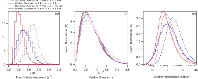
Figure 6 shows distributions of Brunt–Väisälä fre-quency, vertical shear, and Richardson number for points inside (solid) and outside (dashed) overturns in both the upper (red) and lower (blue) free troposphere. Within overturns, the static stability is significantly reduced when compared to normal conditions (Fig. 6a). Of course, this may be partly due to the turbulence it-self. However, here the Brunt–Väisälä frequency is
computed on the monotonic reordered potential tem-perature profile, which we presume to be representa-tive of the turbulent environment. Therefore, no unstable profile enters these statistics. In comparison, there is hardly any change in the distributions of ver-tical shear except a tendency to observe stronger shear outside of overturns in the upper troposphere (Fig. 6b). Thus, stability changes may account for the changes in Richardson number (Fig. 6c) that exhibit smaller values within the overturns. Interestingly, Richardson numbers are weaker in the upper troposphere outside of the overturns, indicating that turbulence is more likely to occur there than in the lower troposphere. It is well known that GWs are phenomena that can locally reduce the static stability or even overturn and lead to turbulence, as inferred from theoretical considerations by Hodges (1967), Chao and Schoeberl (1984), and
Fritts and Dunkerton (1985)and as shown in observa-tions byFritts et al. (1988b). These studies showed in particular that turbulence is localized in the portion of the wave characterized by reduced static stability rather than in portions characterized by large shear.
4. Link between turbulence and GW over the Indian Ocean
Figure 7illustrates the Thorpe analysis and its link with the variability of the environment for Gan Atoll FIG. 5. Mean profiles (black) and standard deviation (gray shading) of (a) potential temperature (K), (b) Brunt–Väisälä frequency (s21),
(c) horizontal wind speed (m s21), and (d) vertical shear (s21) for the whole dataset.
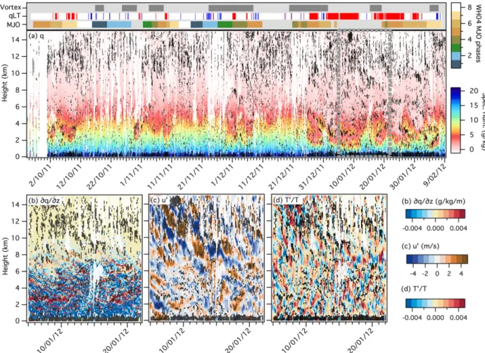
during C/D.Figure 7ashows the time–height evolution of turbulent regions and its relation to specific humidity for the whole observation period. Consistent with
Fig. 4c, turbulent regions are most frequent in the planetary boundary layer and in the upper troposphere. In the lower free troposphere (1–7 km), turbulence is more intermittent with higher frequency during rela-tively dry periods (e.g., 2–12 and 30–31 October, 30 November–8 December, and from 26 December until the end of the observation period). Another example is given byBellenger et al. (2015b, their Fig. 1), suggesting that this is a robust feature of turbulence in the lower troposphere above tropical oceans. The three other panels ofFig. 7focus on the 5–22 January dry period (gray frame onFig. 7a).Figure 7bsuggests some link between turbulence and moisture vertical gradients below 8-km height already noted by Bellenger et al. (2015b). These anomalous moisture vertical gradients are comparable to those observed byLuce et al. (2010b)
andDavison et al. (2013b,c) and are characterized by vertical scales ranging from a few hundreds of meters to 1 km (thus a wavelength of up to 2 km). This link be-tween the occurrence of turbulence and finescale mois-ture variations is visible in particular during 5–10 and 18–22 January around 3–4 km and during 10–18 January between 6- and 7-km heights.
Internal GWs typically have vertical wavelengths of a few kilometers in the troposphere (e.g., Fritts et al. 1988a; Tsuda et al. 1994b; Shimizu and Tsuda 1997;
Reeder et al. 1999;Lane et al. 2003;Leena et al. 2012;
Hankinson et al. 2014a). InFigs. 7c and 7d, the pertur-bations of zonal wind and normalized temperature for the same dry period are shown (refer to section 2b). Distinct variations, which can be interpreted as a GW
signature, are visible on both panels. Up- and downward phase propagation can be seen. These features are consistent with observations reported by Tsuda et al. (1994b)above the mountainous island of Java, for ex-ample. Turbulence appears to be associated with these perturbations and can be observed between strong zonal wind or temperature anomalies from 12-km height on 10 January and gradually downward to 9-km height on 15 January (Figs. 7c,d). Note, however, that wind and temperature perturbations are not always clearly asso-ciated with one another. An example can be seen be-tween 4- and 8-km heights from 10 to 12 January: there is a clear downward phase propagation in zonal wind anomalies (Fig. 7c) and an upward one in temperature perturbations (Fig. 7d).
Figure 3shows the mean vertical power spectra for zonal and meridional wind perturbations, balloon ascent rate, GW normalized temperature, and specific humid-ity anomalies computed on the profiles processed using the Lane et al. (2003) approach (see section 2c). The spectra of zonal and meridional wind peak at 7.5-km vertical wavelength, while temperature and moisture spectra peak around 3–5 km. The vertical ascent rate spectrum also exhibits a maximum around 2–3 km, but with a relatively flat spectrum. These spectra are con-sistent with previous studies (Fritts et al. 1988a;Reeder et al. 1999; Gong and Geller 2010; Hankinson et al. 2014a) and, in particular, with the fact first discussed by
Lane et al. 2003that ascent rate perturbations empha-size waves with shorter vertical wavelength. Spectral maxima for T0and w0are found within the 1–5-km band chosen for GW filtering.
Composited GW perturbations (X05 u0, y0, w0, T0/T, and q0) are obtained using either maxima in normalized FIG. 6. Distribution of (a) Brunt–Väisälä frequency (s21), (b) vertical shear (s21), and (c) gradient Richardson number inside (solid) and
outside (dashed) the overturns for the lower troposphere (blue) and the upper troposphere (red).
APRIL2017 B E L L E N G E R E T A L . 1259
temperature 1–5-km filtered perturbations, (T0/T )f,
(GWT;Fig. 8), or maxima in ascent speed 1–5-km filtered perturbations, w0f (GWw; Fig. 9) as reference heights. Only (T0/T)fand w0f perturbations having peak-to-peak
variations of more than two standard deviations were used. Each GW perturbation is normalized so that the apparent vertical wavelength for reference profile, either (T0/T)for w0f, is 1.Figure 10shows the distributions of
apparent vertical wavelengths and of the corresponding altitudes of the perturbation maxima used to compute the composited GWs. Note that no attempt is made to sep-arate downward- and upward-propagating waves.
Figure 8a shows composites based on GW filtered normalized temperature perturbations (T0/T )f (GWT;
green line). These events most commonly correspond to apparent vertical wavelengths between 2 and 3 km (Fig. 10a, green). They are more frequent in the lower troposphere (Fig. 10b, green), where the stability is
higher (Fig. 5). Dynamical perturbations in phase quad-rature are associated with these tempequad-rature variations. In particular, it is interesting to note that, even if no particular selection was made concerning the relationship between (T0/T) and u0, the zonal wind perturbation would reach 1 m s21 amplitude above the temperature maxi-mum perturbation. Note that this phase relationship is even clearer when considering composited u0f (not shown). On the other hand, meridional wind perturba-tions do not survive this composite procedure. Indeed, 60% of the selected (T0/T )fperturbations correspond to
u0f(1/2). 0, and 40% to u0f(1/2), 0, whereas no such asymmetry is apparent for meridional wind perturba-tions. The reason for this may be linked to the dominance of certain types of Kelvin waves in the GWT ensembles. However, a detailed study of the wave types involved in this composite is beyond the scope of this article and must be reserved for future work.
FIG. 7. (a) Time–height plot of turbulence occurrence (black segments) and specific humidity (g kg21; colors) for the whole observation period based on Gan soundings during C/D. Bar graphs above (a) indicate the following: (top) vortex presence (gray) within 208S–08, 608–1008E (refer toFig. 1); (middle) driest (red) and wettest (blue) periods; and (bottom) MJO phase evolution (by color) for MJO amplitude. 1 as defined byWheeler and Hendon (2004). (b) Specific humidity vertical gradients (g kg21m21), (c) zonal wind filtered perturbations u0f(m s21), and (d) normalized temperature filtered perturbations (T0/T )ffor the 5–22 Jan 2012 period [marked by the gray
frame on (a)]. Cloudy regions in (a) and (b) are shaded in white.
Ascent rate perturbations, which are linked to vertical wind variations, have mean amplitude of less than 0.1 m s21 and peak in between temperature and zonal wind perturbations. This suggests that the composites are indeed representative of GW activity (e.g.,Holton 2004). Interestingly, these composites are associated with large variations in specific humidity. The observed moisture variations of about 0.5 g kg21 are negatively correlated with temperature (and thus roughly in phase with density variations). These variations are primarily due to GW signal in the lower troposphere (mean am-plitude of about 1 g kg21, not shown), but such a signal is also observed in the upper troposphere with weaker amplitude (less than 0.1 g kg21, not shown). Therefore, the moisture layers detected byLuce et al. (2010a)and
Davison et al. (2013b,c) and the associated moisture gradients [Fig. 7bandBellenger et al. (2015b)] could be partly associated with GW activity.
Figure 8b shows the associated average profiles of turbulence percentage, cloud fraction, and Richardson number. There is a clear modulation of turbulence fre-quency (from less than 5% to close to 25%) associated with these GWs and corresponding to small Richardson
number. The turbulent fraction is in phase quadrature with temperature and moisture perturbations and in phase with zonal wind perturbations (Fig. 8a). Turbu-lence is associated with strongly negative vertical tem-perature gradients and strongly positive moisture gradients. This phase relationship between turbulence frequency and temperature perturbations is common for all altitudes, but the turbulence profile shows peak-to-peak variations of slightly more than 10% in the lower troposphere and of about 30% in the upper troposphere (not shown). Interestingly, these GW perturbations are associated with a minimum in cloud fraction. Yet this fraction rises quickly above the turbulence maximum (especially in the lower troposphere), suggesting that turbulence often occurs near the cloud base, either for the stratiform extension of a convective system (Luce et al. 2010b), altocumulus (Wilson et al. 2014;Worthington 2015), or cirrus (Luce et al. 2010c).
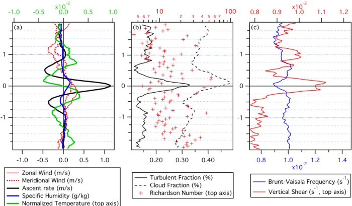
To better understand the processes at work in turbu-lence generation by GWT with strong temperature sig-nature,Fig. 8cshows the associated mean variation of the Brunt–Väisälä frequency and vertical shear of the horizontal wind. Both are negatively correlated with FIG. 8. Composites based on normalized temperature filtered perturbations (T0/T )fof (a) unfiltered perturbations of zonal wind u0(m s21;
red solid), meridional wind y0(m s21; red dashed), balloon ascent rate w0(multiplied by 5; m s21; black), normalized temperature T0/T (green; upper axis), and specific humidity q0(g kg21; blue); (b) raw turbulent fraction (black solid), cloud fraction (black dashed), and Richardson number (red crosses; upper axis); and (c) raw Brunt–Väisälä frequency (s21; blue) and vertical shear (s21; red; upper axis). Note that the vertical axis is in number of wavelengths. Perturbations are defined by removing a 5-day mean. Filtered perturbations are obtained by applying a low-pass filter removing wavelengths smaller than 1 km and removing a cubic fit and a 5-km boxcar (seesection 2cfor details).
APRIL2017 B E L L E N G E R E T A L . 1261
turbulence frequency (Fig. 8b) with amplitudes on the order of 25% and 15% of their mean values, re-spectively. Turbulence is associated with a stability minimum, a wind speed maximum (Fig. 8a), and a ver-tical shear minimum (Fig. 8c). Maximum vertical shear values are found above and below, as in the case pre-sented byWilson et al. (2014). Note that this result does not guarantee that turbulence arises from the convective breaking of these GWTs (GWT-induced static in-stability). One reason is that the clear-air troposphere is statistically stable, and large temperature perturbations are thus needed to create unstable regions. This was not the case for previous studies considering the isothermal upper atmosphere (Hodges 1967;Chao and Schoeberl 1984;Fritts and Dunkerton 1985;Fritts et al. 1988b). Yet the change in stability associated with these waves may play a role in triggering turbulence. As discussed, for instance, by Worthington (2015), even if the tempera-ture variation is not sufficient to induce convective in-stability and wave breaking, it can still reduce the stability enough so that even the average shear is suffi-cient to induce Kelvin–Helmholtz instability. This would be consistent with results fromFritts and Rastogi (1985)who found that lower frequency GWs are more likely to give rise to Kelvin–Helmoltz instability.
Figure 9ashows composites based on vertical ascent rate perturbations (black line). Corresponding apparent
vertical wavelength and vertical position distributions are given inFig. 10(in black). Consistent with previous studies (Lane et al. 2003; Gong and Geller 2010;
Hankinson et al. 2014b), GWws correspond to shorter vertical wavelengths (many events with 1–2-km wave-lengths) and thus higher frequencies (Fig. 10a). This confirms that the two GW ensembles, GWT and GWw, based on selection on temperature and ascent rate per-turbation, respectively, are depicting different cases even if the two might not be entirely distinct. In contrast to the GWTs (green), these GWws tend to be more active in the upper troposphere (Fig. 10b). The com-posite onFig. 9ashows large variation in ascent rate with an amplitude of 1.2 m s21. The phase relationship be-tween the ascent rate and the temperature variations is the same inFigs. 8aand9a. Yet the signatures in hori-zontal wind and specific humidity are weaker. The weaker moisture perturbation can be partly explained by the relatively higher proportion of events diagnosed in the upper troposphere for GWws (60%) compared to GWTs (35%; see Fig. 10b). As in Fig. 8, maximum in turbulence (35% due primarily to GWs in the upper troposphere, not shown) stands just below an increase cloud fraction and is associated with maximum ascent rate perturbation and with smaller Richardson number (Figs. 9a,b). Figure 9c shows that, for these higher-frequency GWs, maximum turbulence higher-frequency is FIG. 9. As inFig. 8, but with composites based on balloon vertical ascent rate filtered perturbations wf0.
associated with maximum vertical shear and a decrease in static stability. This could reflect the fact that higher-frequency GWs tend to break because of both dynami-cal and convective instabilities, as shown byFritts and Rastogi (1985). However, the decrease in static stability is weak (;10%), which suggest that turbulence is more likely to occur due to dynamical instability. In addition, one can note that these GWws have vertical wave-lengths that are comparable to the vertical extent of observed Kelvin–Helmholtz billows (;1 km or more; seeLuce et al. 2010c), which are also characterized by a strong signature in vertical wind.
Daily average indices of turbulence and GW activity (GWT based on normalized temperature and GWw based on vertical ascent) are computed for both the
lower and upper troposphere. The only significant cor-relation is found in the lower troposphere between tur-bulence and GWT indices, where their activity is the strongest (Fig. 10b). When daily averages for both in-dices are computed using all eight 3-hourly radiosondes (168 days), the correlation is 0.66. When at least four soundings per day can be used (337 days), the correla-tion is 0.52. In the upper troposphere, no such re-lationship can be found, perhaps because of a greater role of other turbulence sources, such as evaporative cooling at cloud base (Luce et al. 2010c;Wilson et al. 2014), given that clouds are more frequent at these al-titudes (e.g.,Figs. 2c,7a).
Finally, note that when constructing our composites on zonal wind perturbations (GWus), we obtain structures FIG. 10. Distributions of (a) vertical wavelengths for the GW cases selected on normalized temperature (T0/T )f
(green) and balloon ascent rate w0f(black) used to construct composites inFigs. 8and9, respectively, and (b) the
reference altitudes (corresponding to 0 on theFigs. 8and9composite’s vertical axis).
APRIL2017 B E L L E N G E R E T A L . 1263
that are consistent with the classical view of GWs, similar to what is seen inFig. 8a(not shown). Furthermore, these GWus are characterized by larger vertical wavelength, ranging from 2 to 4 km with a clear peak at about 3 km, as predicted byLane et al. (2003). They are primarily ob-served in the upper troposphere (not shown). Yet the associated turbulent fraction variations are weaker (;5%). This suggests that either these low-frequency GWus do not usually break in the troposphere or that the localization of turbulence in a particular phase of these waves is very weak.
5. Link with the tropical variability
The focus of this section is the link between GWTs and GWws juxtaposed with local and regional convec-tive activity. However, it should be noted that other sources, such as the jet stream, might have an influence on GW activity, even in this region of the equatorial Indian Ocean. Previous studies already reported higher-frequency/shorter-vertical-wavelength GWs in the di-rect environs of convective clouds (e.g.,Lane et al. 2003;
Gong and Geller 2010;Dhaka et al. 2011;Hankinson et al. 2014b). The present dataset differs from these previous ones, since it represents an open-ocean envi-ronment far away from any significant topography.
Figure 11shows scatterplots of daily GW activity indices (GWT based on temperature and GWw on vertical as-cent rate) in the lower and upper troposphere as a function of the C-band radar–derived daily average echo-top height for C/D observation sites (Xu et al. 2015). It is clear that GWTs characterized by a strong signal in temperature are negatively correlated to local convective activity in both the lower troposphere (Fig. 11c) and in the upper troposphere, although the correlation is not significant (Fig. 11a). This is possibly because these longer-wavelength GWs can travel far-ther away from their source in a stable environment and thus are more active in calm regions away from con-vective sources. These waves could also be associated with frontal structures, for example, because of in-trusions of dry air into the ITCZ, which are observed in this region (Kerns and Chen 2014). In contrast, short GWws are positively correlated with local convection (Figs. 11b,d) with a higher correlation coefficient in the upper troposphere. This is consistent with previous studies, such as Dhaka et al. (2011), which showed shorter-wavelength GWs in the upper troposphere as being associated with local convection. This is also consistent with observations reported by Hankinson et al. (2014b), although they focus on stratospheric GWs at higher altitudes. Thus, depending on convective ac-tivity, the characteristics of GWs change with more GWs
having larger vertical wavelengths (within the 1–5-km band) during suppressed conditions and shorter ones during active convection.
The link between turbulence and moisture in the lower troposphere that is visible onFig. 7ahas also been discussed inBellenger et al. (2015b). The dry intrusion over Gan Island on 30 November described by Kerns and Chen (2014)is the beginning of a long period of dry conditions over the equator that lasts throughout De-cember and January (Fig. 7a). Figure 12a shows the distribution of lower-tropospheric moisture and the threshold used to define dry and wet conditions (time series reported onFig. 7a).Figure 12further shows the sensitivity of GW activity and turbulence characteristics to this criterion in the lower troposphere. The activity of GWTs is greater in dry conditions (Fig. 12b), whereas the opposite is observed for the shorter GWws (Fig. 12c). This is consistent with long GWTs found in stable envi-ronments associated with dry conditions and with short GWws directly linked to local convective activity. Finally, turbulence is stronger during dry conditions compared to wet conditions (Fig. 12d). Note that these results are tightly linked to Fig. 11, as the driest conditions corre-spond to low convective activity, whereas humid ones correspond to more convection.
Tropical depressions (TD) and cyclones are associ-ated with organized convective systems that are well-known sources of inertia–GWs (e.g.,Ki and Chun 2010).
Figure 13 is a simple diagnostic showing the distribu-tions of the standard deviation of normalized tempera-ture perturbations (the GWT activity index) depending on the presence (or lack) of TDs close to the observation sites (as defined by the gray frame onFig. 1). The time series of this TD index is also reported onFig. 7a(gray bars on the top) together with other indices. TDs are present during any phase of the MJO in this example. Yet a more precise analysis reveals that the MJO does indeed modulate the number of TD initiations (Duvel 2015). Clearly, GWT activity increases when a TD is present in the vicinity. No such difference is noted on GWw activity. This does not prove that the increase of GWT activity is only related to TDs, since GWT may have other sources (such as fronts or jet streams), but this stresses that a variety of nonlocal sources of GWTs may have to be taken into account to correctly trace the source(s) of turbulence.
As local and surrounding convection can affect tur-bulent generation through modulation of GW activity, large-scale climate phenomena such as the MJO should also have an impact on turbulence occurrence and origin over the Indian Ocean. Considering the observation sites’ locations (Fig. 1), MJO phases 1–4 correspond to convectively active periods and phases
5–8 to suppressed periods (Wheeler and Hendon 2004). Indeed, dry conditions are usually observed during phase 5–8 of the MJO over Gan Island (Fig. 7a).
Figure 14shows the degree of activity of long GWTs and short GWws and of turbulence in the lower and
upper troposphere as a function of MJO phase. In both the lower and upper troposphere, GWTs are the most sensitive to MJO phase with maximum activity during phases 4–7 (Fig. 14a), when convection moves east away from the observation sites in the Indian Ocean FIG. 11. Scatterplots of daily (a),(c) GWT and (b),(d) GWw activity indices (filtered perturbation standard
deviation for normalized temperature and vertical ascent rate, respectively) for the upper (red) and lower (blue) troposphere as a function of daily average echo top observed during C/D from Gan, R/V Mirai, and R/V Revelle (Xu et al. 2015, their Fig. 7). The daily GW activity indices are computed only using days with eight values of GW. Linear correlation coefficients and the numbers of days used for the computation are also indicated. Underlined correlation coefficients are significant at the 99% level.
APRIL2017 B E L L E N G E R E T A L . 1265
[see Fig. 1 and Wheeler and Hendon (2004)]. Short GWws have maximum activity in the upper tropo-sphere during phases 2–6 (Fig. 14b), corresponding to both active and suppressed phases of the MJO. Tur-bulent fraction variation with MJO phase is also evi-dent in the lower and upper troposphere (Fig. 14c). Turbulent fraction peaks during phase 6 (dry condi-tions) in the former case and during phase 3 (convec-tive conditions) in the latter case, although it is difficult
to simply attribute these peaks to maxima in GWT and GWw activity.
6. Summary and discussion
This article presents a statistical analysis of tropo-spheric turbulence in a tropical open-ocean region based on a large dataset of radiosondes (more than 3500 soundings from the MISMO, CIRENE, and C/D FIG. 12. (a) Frequency of occurrence of the mean 2–4-km-height mixing ratio (g kg21) for the entire dataset together with the threshold to define dry (red) and wet (blue) conditions (vertical lines). Normalized distributions of the (b) GWT activity index and (c) GWw activity index and (d) the turbulent fraction in the lower troposphere. Red and blue distributions correspond to dry and wet conditions, re-spectively. The black distribution corresponds to all conditions. GWT (GWw) activity is measured by the standard deviation of nor-malized temperature (balloon ascent rate) filtered perturbations. In (b),(c), and (d), the blue and red distributions are found significantly different to the 99% level by using a x2two-sample test.
FIG. 13. Normalized distributions of GWT activity in the lower troposphere (1–7 km) when a vortex is present in 208S–08, 608–1008E (blue) or absent (red). Vortices are selected fol-lowingDuvel (2015). GWT activity is measured by the standard deviation of normalized temperature filtered perturbations. The two distributions are significantly different to the 99% level using a x2two-sample test.
campaigns), which confirm and extend the study of
Bellenger et al. (2015b). Turbulent regions extending from 40 to 1000 m in the vertical are observed, corre-sponding to eddy diffusivities on the order of 1–100 m2s21. These values are obtained making some assumptions about the link between the Thorpe and the Ozmidov length scales (e.g., Schneider et al. 2015; Fritts et al. 2016). We note that Thorpe analysis based on regular radiosondes may miss the smallest turbulent regions, while potentially creating unrealistically large regions by merging neighboring small ones (Wilson et al. 2013). Part of the largest turbulent regions detected here may result from several smaller overturns, leading us to be-lieve the tail of the distribution is overestimated. Tur-bulence is most frequent in the upper free troposphere near 12-km height, with larger vertical extents than those in the lower troposphere. Yet, because of the relatively lower stability in the upper troposphere, eddy diffusivities are comparable in both domains. Further-more, turbulence clearly corresponds locally to weaker stability than for the surrounding environment but not to stronger vertical shear. This suggests a role for GWs in the creation of turbulence based on past theoretical works (Hodges 1967;Chao and Schoeberl 1984;Fritts and Dunkerton 1985) and observations (Fritts and Rastogi 1985;Fritts et al. 1988b).
The link between turbulence and GWs is then further investigated. The GW signals with apparent vertical
wavelengths of 1–5 km are detected in the filtered per-turbations of horizontal wind, temperature, and balloon vertical ascent profiles. Composites are constructed based on strong variations in each of these parameters that correspond well to GW structure. Consistent with
Lane et al. (2003) and Geller and Gong (2010), hori-zontal wind variations are associated with larger ap-parent GW vertical wavelengths, ascent rate with shorter ones, and temperature in between. While no clear link such as spatial phase locking is found between turbulence and GWs isolated from their signature in horizontal wind, there is however a clear modulation of turbulence occurrence by GWs with strong signal in temperature and vertical ascent rate. The former are mainly detected in the lower troposphere, whereas the latter are mainly detected in the upper troposphere.
Some notable differences in the link between turbu-lence and GWs are found for short GWws and long GWTs. For GWTs, turbulence appears in conjunction with negative GW anomalies in the temperature gradi-ent (a decrease in stability) and with maximum hori-zontal wind (a minimum in vertical shear), as predicted by theory (Hodges 1967; Chao and Schoeberl 1984;
Fritts and Dunkerton 1985) and observed in cases studies (Fritts et al. 1988b;Wilson et al. 2014). Turbu-lence may thus sometimes result from convective in-stability alone, but, more generally, both in-stability reduction by the GWs and vertical shear may generate FIG. 14. Mean (a) GWT and (b) GWw activity and (c) turbulent fraction as a function of theWheeler and Hendon (2004)RMM index MJO phase (for index amplitude higher than 1). GWT (GWw) activity is measured by the standard deviation of normalized temperature (balloon ascent rate) filtered perturbations. Red (blue) is for upper (lower) troposphere. Error bars represent the t-based 99% confidence interval for the means.
APRIL2017 B E L L E N G E R E T A L . 1267